Moment-based Bayesian Poisson Mixtures for inferring unobserved units
Abstract
We exploit a suitable moment-based characterization of the mixture of Poisson distribution for developing Bayesian inference for the unknown size of a finite population whose units are subject to multiple occurrences during an enumeration sampling stage. This is a particularly challenging setting for which many other attempts have been made for inferring the unknown characteristics of the population. Here we put particular emphasis on the construction of a default prior elicitation of the characteristics of the mixing distribution. We assess the comparative performance of our approach in real data applications and in a simulation study.
1 Introduction
We consider the problem of inferring the total number of units in a finite population in the presence of count data where during an experiment or an observation stage all the units are potentially observable multiple times but only those who are observed at least once are in fact enumerated in the sample. This setting is of interest in wildlife conservation when one is willing to infer on the number of yet unobserved animals living in an area using the information coming from the repeated detection of the observed units. The same setting occurs in many other fields such as in social sciences where the actual size elusive populations needs to be properly assessed (Böhning and van der Heijden, 2009), in software reliability (Lloyd et al., 1999), in genomics (Wang et al., 2005), biology (Guindani et al., 2014) and linguistics (Efron and Thisted, 1976). In ecology the same type of problem, known as species richness problem (Bunge and Fitzpatrick, 1993; Chao and Bunge, 2002; Wang and Lindsay, 2005; Chao and Chiu, 2016) has received a lot of attention and many alternative models and methods have been proposed.
Let us fix our model setup. Let denote the finite size of the population of interest. Indeed it is important to clarify from the outset that in the species sampling terminology is the number of distinct species and not the size of the animal/organism population under investigation. In order to avoid restrictive homogeneity assumptions we can assume that all units act independently from each others conditionally on all the individual detection rates so that the joint count probability can be expressed as follows
where , . However, the individual rate parameters can be thought of as unobserved heterogeneous latent intensities assumed to be drawn from a common distribution . This yields a more flexible hierarchical Poisson mixture distribution for which the probability of observing a single count equal to is
| (1) |
Hence, by exchangeability, the joint probability of observing all the counts of the population , is summarized by the joint probability of the sufficient statistics, called frequency of frequencies,
where represents the number of units whose count corresponds to and . Notice that the number of units with count equal to zero is not available to the observer and is in fact in one-to-one relation with given since
Hence, estimating the main parameter of interest is equivalent to estimating the number of unobserved units. In this hierarchical formulation the likelihood function can be written as follows
| (2) |
where and is the mixing distribution for . In the literature alternative mixtures of Poisson distributions with different finite (Pledger et al., 2003) or continuous (Böhning et al., 2005a) parametric mixing distribution have been considered as well as other nonparametric likelihood-based estimates Norris and Pollock (1998); Wang and Lindsay (2005). In 2010, Wang (2010) proposed to consider a Poisson compound gamma model estimating the mixture by a nonparametric penalized maximum likelihood approach using a least-squares cross-validation procedure for the choice of the common shape parameter. Other approaches which are worth mentioning are the Abundance-based Coverage Estimator (ACE), lower bounds and their variants (Chao and Lee, 1992; Mao, 2006). From the Bayesian perspective relevant recent references for the parametric approach are Barger and Bunge (2010) and Guindani et al. (2014) from the nonparametric perspective. A rather different sampling perspective stemming from the species sampling sequential approach has been put forward in Lijoi et al. (2007) and, more recently, in Zhou et al. (2017). Notice however that in Lijoi et al. (2007) the size of the population is indeed assumed to be infinite. Differently from Guindani et al. (2014) where a nonparametric Dirichlet process prior is used for the nuisance our proposal yields an alternative nonparametric estimate of the population size based on the likelihood in (2) reparameterized in terms of a finite number of moments of a suitable mixing distribution as illustrated in the next section.
2 Moment-based mixtures of truncated Poisson counts
To begin with
we show that,
in order simplify our task,
(2) can
be approximated arbitrarily well by a model in which
the mixing distribution has a compact support in
for a suitable choice of .
In fact, the following holds:
Theorem: Let be a generic probability distribution with support on ; such that
where is the distribution restricted to have compact support on
proof: In order to prove the theorem we have to verify that
where is the Borel -algebra. Since
| (3) |
and
| (4) |
we have
Moreover, from (3) and (4) it follows that
This minimal restriction on a compact support of the mixing distribution allows us to consider the one-to-one correspondence of a compact supported univariate distribution and the infinite sequence of its moments. In fact, we can simplify the functional form of the likelihood as a function of a finite number of characteristics of . To make it explicit we will be using first another one-to-one mapping between finite measures
so that we can eventually regard the likelihood as a function of a finite number of moments of the finite measure uniquely corresponding to . Hence, for a fixed value , we can always consider the following simplified parametric model for the probability of each frequency counts
| (5) |
where is the -th ordinary moment corresponding to the finite measure not necessarily with total mass equal to 1. Indeed we can derive the corresponding likelihood
| (6) |
which can be thought of
as an approximate version of the original mixture of Poisson
model
(2).
This suggests that the
representation of the original model
in terms of an infinite-dimensional functional parameter
will be amenable to a
flexible finite dimensional representation.
This will ease the task of
implementing a default Bayesian approach for
making inference on the parameter of interest .
Indeed, in order to further simplify the likelihood structure and represent its
expression as a function of the moments of a
probability measure (with fixed total mass equal to 1)
supported on
we will consider the following trick:
we take the normalized
probability distribution
corresponding to , namely
so that
It is immediate to realize that since we get
so that, summing up over all the normalizing constant is such that
One can replace the use of with and escape from the infinite summation defining from the latter expression a convenient further approximation which represents a flexible parametric distribution for the frequencies of counts as follows
| (7) |
where the probabilities are expressed as a function of the first moments of the probability distribution
where
Usually but the parametric model is still well defined also for . However, we point out that for the structure of the likelihood function (2) there is information only for the first moments of the mixing distribution. The resulting model likelihood will be represented as
| (8) |
and it can be considered a convenient approximation of (6) and hence of the original nonparametric model (2). We can make a final simplification by separating the dependence of from and the moments of a single probability distribution supported on namely
| (9) |
which corresponds to the change of measure for due to a scale factor for the rate parameter . In the following we will use the notation instead of and will be the vector of the first moments of an arbitrary probability distribution supported on . We can then express our flexible parametric model in terms of a vector of parameters so that
| (10) |
where the - truncated moment space is such that
where is the class of probability distributions with support in . The ordinary moment space is a constrained -dimensional convex body and hence it is not easy to deal with. As proposed in Tardella (2002) and also used in Tardella and Farcomeni (2008) in the context of the discrete-time capture-recapture experiments one can also consider a further reparameterization of in terms of the so-called canonical moments (Skibinsky, 1986; Dette and Studden, 1997). We define the -truncated moment class of distributions
where . Moreover, we define the following quantities
The generic element of is defined as follows
so that can be any point in the space . Then one can do all the computations and simulations in this unconstrained parameter space and finally reparameterize back into the space of the ordinary moments with little extra effort so that MCMC approximations of the posterior distribution can be safely derived. In order to implement a fully Bayesian approach we need to set up a suitable prior distribution for the vector of parameters involved in the model. In the next section we will give details on how one can elicit a suitable default prior distribution on the moment space .
3 Default Bayesian inference
In order to implement a fully Bayesian approach for (10) we need to elicit
the joint prior distribution for the whole parameter vector ().
We first show how a principled default Bayesian inference
can be derived for model (10) based on
the count frequency probabilities .
We note that, for fixed values of the parameters and taking the expression in (10) is a multinomial likelihood in terms of the probabilities which are in turn one-to-one related to . This allows us to consider a standard Jeffreys’prior on and transform it back in terms of a default distribution on conditionally on any fixed value of and , taking into account the appropriate Jacobian. It is known that the Jeffreys’prior for an unconstrained multinomial parameter vector is a Dirichlet distribution and one can argue that for the count frequency probabilities which are constrained on a proper convex body contained in the -dimensional simplex the same functional form of the Jeffreys’ prior is preserved up to a different normalizing constant. So we have
| (11) |
As previously mentioned simulation within the moment space can be eased by reparameterizing the ordinary moments of the distribution in terms of the corresponding canonical moments (Tardella, 2002). The only step needed to re-express our Jeffreys prior in terms of is the evaluation of the appropriate Jacobian. Indeed, to simplify formulae, let us denote with , , and . The count frequencies in (7) can be expressed as a function of :
as follows
where stands for the denominator. Notice that both vectors and can be completed when needed by and using the known constraints: and . Hence we have that the standard Jeffreys’prior on multinomial cell probabilities is
and the corresponding Jeffreys’prior in terms of can be written as
| (12) |
where is the Jacobian matrix containing the partial derivatives of . The Jacobian matrix has the extra-diagonal elements
while the diagonal elements are
Now we finally express the Jeffreys’prior in terms of using (12) and the one-to-one mapping (9) which maps into
and hence we have
where is easily to derived as follows
To complete the prior elicitation for our model we consider for
three different non-informative prior distributions:
uniform, and Rissanen’s prior.
We will investigate the sensitivity of the posterior analyses and compare its performances
by simulation study and results of some real data examples.
Notice that so far we have assumed a fixed upperbound for the support of
the mixing distribution of .
Now we need to endow with a prior distribution.
Indeed considering how we jointly rescale all the moments of
into the moments of
we use as a reference distribution
| (13) |
In order to avoid an improper distribution and degenerate inference for we fix a positive lowerbound () for the support of .
4 Applications
4.1 Application to Simulated data
In order to evaluate the performance of our proposal we implemented a simulation study according to the same setting considered in Wang (2010) as described in Table 1.
| Setting | Distribution () | |
|---|---|---|
| Gamma | ||
| 1 | 0.90 | |
| 2 | 0.59 | |
| 3 | 0.20 | |
| Gamma Mixture | ||
| 4 | 0.65 | |
| 5 | 0.57 | |
| Log-Normal | ||
| 6 | 0.82 | |
| 7 | 0.50 | |
| 8 | 0.36 | |
| Log-Normal Mixture | ||
| 9 | 0.61 | |
| Finite Mixture | ||
| 10 | 0.8 | 0.76 |
| 11 | 0.89 | 0.46 |
| 12 | 0.8 | 0.29 |
For each setting a different mixing distribution on the Poisson intensity is fixed and 100 simulated datasets are drawn and used to repeat the estimation procedure. Bias and mean square error of point estimates and coverage of interval estimates are approximatively evaluated averaging the results obtained with the simulated datasets. We compare our method with the recent non parametric approach based on a penalized likelihood proposed in Wang (2010) which highlighted inferential difficulties of the previously available approaches and showed a substantial improvement over the latter. Wang’s procedure is implemented in the R package SPECIES (Wang, 2011) where the corresponding function is named pcg(…). The package allows also to compute point and confidence interval estimates from alternative nonparametric and semi-parametric methods using the first counts observed. In order to make a sound comparison with Wang’s procedure we fixed the number of moments of the probability distribution considered to be since in Wang’s simulation study only the first 10 counts are considered. Although we evaluated several prior choices for we report in Table 2 only the results obtained from the uniform prior which leads to the best performances. We will denote by the resulting estimator.
| Setting | Setting | ||||||||
|---|---|---|---|---|---|---|---|---|---|
| 1 | 1020 | 27.93 | 100 | 2 | 1135 | 160.73 | 99 | ||
| 1020 | 28.11 | 97 | 1138 | 161.00 | 99 | ||||
| 1011 | 28.39 | 95 | 1014 | 149.47 | 99 | ||||
| 3 | 1070 | 147.85 | 100 | 4 | 1009 | 58.08 | 100 | ||
| 1034 | 133.25 | 100 | 1013 | 59.16 | 100 | ||||
| 924 | 234.71 | 100 | 991 | 124.47 | 99 | ||||
| 5 | 1041 | 72.02 | 100 | 6 | 1004 | 106.64 | 100 | ||
| 1040 | 72.42 | 100 | 997 | 102.60 | 100 | ||||
| 1009 | 160.21 | 96 | 1041 | 113.63 | 98 | ||||
| 7 | 829 | 171.03 | 83 | 8 | 907 | 113.89 | 100 | ||
| 831 | 169.51 | 86 | 912 | 115.77 | 100 | ||||
| 996 | 198.86 | 97 | 1016 | 197.61 | 99 | ||||
| 9 | 976 | 71.94 | 98 | 10 | 1117 | 122.48 | 72 | ||
| 974 | 71.88 | 97 | 1061 | 78.02 | 88 | ||||
| 1028 | 163.07 | 100 | 1038 | 56.93 | 83 | ||||
| 11 | 1207 | 281.11 | 91 | 12 | 880 | 154.43 | 100 | ||
| 1192 | 276.01 | 91 | 879 | 153.87 | 100 | ||||
| 1035 | 177.26 | 87 | 938 | 169.39 | 93 |
As we can see from the results in Table 2 graphically summarized in Figure 1 our Bayesian estimators seem to compete well with Wang’s pcg procedure although occasionally they can be beaten in terms of efficiency and interval coverage. In his paper Wang shows how his estimator almost uniformly outperforms all previously available estimators in terms of precision and coverage. We find out that a slight modification of the fully Bayesian recipe can do even better. It turns out that integrating out the following penalized likelihood
with the
similar prior choices for and and a uniform measure on the
moments one gets a better performance as we can see in
Figure 2.
However, we will not consider it further because it does not correspond to a fully Bayesian approach.
Moreover, even though our new methods (fully Bayesian and penalized integrated
likelihood) are computationally intensive,
the derivation of the interval estimates is often quicker
compared to Wang’s pcg procedure which relies on a costly double-bootstrap procedure.

Overall if we average on all the twelve simulation settings our turns out to be an improvement over in terms of average mean square error while the corresponding interval estimates show an overall suitable coverage close to the nominal level.
4.2 Real data analyses
We investigate the effectiveness of our proposed estimator with several benchmark datasets used in the recent works of Wang (2010) and Rocchetti et al. (2011) comparing our Bayesian approach with both approaches developed in these papers. The estimator proposed in Rocchetti et al. (2011) is based on a linear regression model on the ratios of successive frequency counts. Namely
We stress that such estimator does not aim to be a flexible nonparametric estimator since it is derived under the assumption that the count distribution belongs to the so called Katz family (Katz, 1952). For this reason we have not used it as alternative competitor in our simulation study. For the following real data Bayesian analyses we will follow the recipe recommended from the simulation study: uniform prior for , Jeffreys’prior on and for we consider the reference prior described in (13).
Traffic data
We start with the famous dataset known as Traffic Data originally studied in Simar (1976) and lately re-analyzed in Böhning et al. (2005b) and Wang (2010). Data are shown in Table 3. They represent the accident counts submitted to La Royale Belge Insurance Company during a particular year. In this example we know the real value for () which is the total number of insurance policies covering both “business” and “tourist” automobiles; hence the complete frequency counts show that the proportion of the unobserved units is very high.
| 1 | 2 | 3 | 4 | 5 | 6 | 7 | n | |
|---|---|---|---|---|---|---|---|---|
| Traffic () | 1317 | 239 | 42 | 14 | 4 | 4 | 1 | 1621 |
For the analysis we have considered all the available positive counts with equal to 7 which is indeed the maximum count observed. The MCMC algorithm runs for 110000 iterations discarding the first 10000. In Figure 3 the trace plots of the three main quantities: , and are shown. It is apparent that there is a strong autocorrelation which is likely yielding a slow mixing of the chain and can affect the resulting Monte Carlo error.
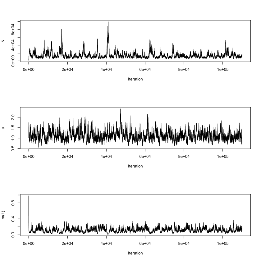
This strong autocorrelation can be due to the strong dependence among the three main quantities as evidenced from the scatter plots in Figure 4 (especially the one corresponding to and ).

However, we have verified that the results do not vary appreciably with a larger MCMC size. Indeed we redraw the acf considering a thin factor leading 2000 iterations. The resulting acf in Figure 5 looks reasonable.
As far as inference on is concerned we can see from the histogram in Figure 6 that the known value is also very close to the mode of the posterior distribution of .
In Table 4 are expressed point and interval estimates from different prior choices of and .
| Methods | |||
|---|---|---|---|
| 9548 | 5642 | 22582 | |
| 9121 | 5416 | 22816 | |
| 8970 | 5662 | 18255 | |
| 6935 | 5121 | 12843 | |
| 7840 | 7742 | 7937 |
As we can see the point estimates are sufficiently stable
with respect to the prior choice strategy.
Moreover our credible intervals always contain the true although the
sensitivity of the upper bound of the credible intervals seems to be
more pronounced than in the case of point estimates.
When we compute alternative estimators
proposed in Wang (2010) and
proposed in
Rocchetti et al. (2011)
we have that both seem to
be more conservative and underestimate somehow the true
( and respectively).
However, in Wang (2010) among many alternative classical procedures
considered in that paper
only the confidence interval derived from
through a double-bootstrap procedure gets the true inside.
Hence we consider our estimator of in this example
one of the few successful estimators
of the quantity of interest, in fact the closest one to the true known value.
Root data
In Table 5 are shown the Root data already analyzed in Wang (2010) which represent the count distribution of the expressed genes of the arabidopsis thaliana in the root tissue. Notice that in this case there is a genuine interest in the unknown number of unexpressed genes since data are collected from a cDNA library sample which, very likely does not allow a full screening of all expressed genes.
| 1 | 2 | 3 | 4 | 5 | 6 | 7 | 8 | 9 | ||
|---|---|---|---|---|---|---|---|---|---|---|
| Root () | 2187 | 490 | 133 | 121 | 37 | 51 | 22 | 19 | 7 | |
| 10 | 11 | 12 | 13 | 14 | 15 | 16 | 17+ | n | ||
| 8 | 6 | 7 | 6 | 4 | 5 | 5 | 18 | 3126 |
Researchers agreed that the arabidopsis thaliana has a relatively small genome with approximatively 27000 protein coding genes not necessarily all expressed in all tissues. This information can be easily exploited in our Bayesian procedure formalizing an ad-hoc prior distribution for by setting a suitable upperbound for the population size of the expressed genes. We fix for our analysis. On the other hand this (a priori) information cannot be employed so easily in the alternative classical approaches.
| Methods | |||
|---|---|---|---|
| 11073 | 8739 | 15316 | |
| 8980 | 8383 | 18771 | |
| 8970 | 8652 | 9288 |
The results of the three alternative procedures are shown in Table 6. As we can see the point estimates and are very close together (8980 and 8870 respectively). As argued in Wang (2010) they could be a conservative estimate of the total number of expressed genes in the root tissue. Our estimate is considerably higher exceeding the value 11000 for both prior choices. Although in this case the population size is not known in advance, however previous works (Ma et al., 2005) suggest a percentage of expressed genes in root tissue greater than 40% of the 27000 protein coding genes and which fits well with the recommendation provided by .
Colorectal polyps
From medical research experiences it is well recognized that diagnosing adenomatous polyps can be subjected to undercount due to misclassification at colonoscopy. We use data from Alberts et al. (2000) where in order to evaluate the recurrence of colorectal adenomatous polyps subjects with previous history of colorectal adenomatous polyps are allocated to one of two treatment groups, low fiber and high fiber. Polyps data-frequency distribution of recurrent adenomatous polyps per patient, by treatment group is reported in Table 7. For both groups the population size is known in advance: 584 for the low fiber treatment () and 722 for high fiber treatment () respectively.
| 1 | 2 | 3 | 4 | 5 | 6 | 7 | 8 | 9 | 10 | 11 | 12+ | n | |
| Polyps low () | 145 | 66 | 39 | 17 | 8 | 8 | 7 | 3 | 1 | 0 | 2 | 3 | 299 |
| Polyps high () | 144 | 61 | 55 | 37 | 17 | 5 | 4 | 6 | 5 | 1 | 1 | 5 | 341 |
In Table 8 are reported alternative point and the interval estimates for both treatments. In this case Wang’s estimator gets closer to the true and also its confidence intervals include the main parameters of interest. Notice that, differently from the other procedures it overestimate the true population size.
| Methods | ||||
|---|---|---|---|---|
| Polyps low | 521 | 410 | 717 | |
| 626 | 424 | 780 | ||
| 492 | ||||
| Polyps high | 544 | 429 | 758 | |
| 806 | 526 | 956 | ||
| 496 | 425 | 567 |
Our proposal, although slightly negatively biased, yields confidence intervals which always contain the true for both data sets and they are also narrower than those resulting from Wang’s approach. Moreover, as we can see from the acf plots in Figure 7 the autocorrelation is sensibly lower with respect to the Traffic data example.
Scrapie in Great Britain (2002-2006)
In Great Britain, scrapie is an endemic fatal neurological disease which affects small ruminants (e.g. sheep, goats etc). In Table 9 is reported the distribution of counts of confirmed scrapie-affected sheep in Great Britain between 2002 and 2006 Rocchetti et al. (2011).
| 1 | 2 | 3 | 4 | 5 | 6 | 7 | 8 | 9 | 10+ | n | |
|---|---|---|---|---|---|---|---|---|---|---|---|
| Scrapie () | 298 | 89 | 42 | 17 | 20 | 7 | 11 | 7 | 3 | 22 | 516 |
For all procedures we consider the truncated distribution of the the first 9 counts while the frequencies corresponding to the counts are summed up to the resulting estimates. As we can see from Table 10 the estimates produced by and are close together (1269 and 1220 respectively). However, our procedure yields wider confidence interval compared with RBB recognizing the possibility of more than 1500 cases of scrapie. On the other hand, the estimates obtained by the Poisson-compound gamma approach of Wang appear much higher than the alternative estimators () and somehow surprisingly high with respect to other recent analyses with the same data set (Böhning et al., 2011). Indeed, the corresponding completeness rate of 25.9% seems to be too low in this case. Notice, however, that the point estimate returned by pcg is not incompatible with our Bayesian inference in terms of its credible interval. On the other hand, the interval estimate returned by pcg function in SPECIES package looks inconsistently beyond the point estimate possibly due to some numerical instability problems.
| Methods | |||
|---|---|---|---|
| 1269 | 890 | 2165 | |
| 1993 | 4312 | 13638 | |
| 1220 | 1151 | 1289 |
Methamphetamine use in Thailand
Data in Table 11 is concerned with the drug abuse in Thailand during the last quarter of 2001. In this table the number of methamphetamine users are displayed for each count of treatment episodes reported by the public health surveillance system.
| 1 | 2 | 3 | 4 | 5 | 6 | 7 | 8 | 9 | 10 | n | |
|---|---|---|---|---|---|---|---|---|---|---|---|
| Methamphetamine () | 3114 | 163 | 23 | 20 | 9 | 3 | 3 | 3 | 4 | 3 | 3345 |
A total of 3345 distinct drug users have been observed with maximum number of captures equal to 10. The count distribution has a very strongly positive skewness: 3114 out of 3345 units present only one capture. This is a clue for a severe undercount or, which is the same, a large frequency of unreported users.
| Methods | |||
|---|---|---|---|
| 55435 | 35472 | 109171 | |
| 55739 | 34783 | 93658 | |
| 61133 | 60986 | 61280 |
The point estimates from Wang and B-B-R are 55739 and 61133 respectively. As reported in Table 12 our point estimate is only slightly lower (). However, similarly to Wang’s procedure, our confidence interval confirms that there can be more than 100000 drug users. Moreover, the lower limits of the of the interval is very close to Chao’s lower bound
which is a conservative nonparametric estimator based on the Cauchy-Schwarz inequality.
5 Final remarks
We have dealt with modeling
individual heterogeneity
within Poisson count distribution in the absence of zero counts.
We developed an original flexible approximation of a mixture
of Poisson distributions where
the mixing distribution is not constrained
to belong to a specific parametric family.
Our Bayesian approach described in Section 2 and 3
is based on a reparameterization of the mixture likelihood function (2) in terms of
the first ordinary moment corresponding to a finite
measure with support where is not necessarily fixed.
In order to obtain
a probability measure
with total mass equal to 1 we have rescaled to and then
we have truncated the infinite sequence of moments of to the first
moments using an explicit renormalization which formally resembles the original likelihood (6).
Moreover, we have exploited the
reparameterization of the ordinary moments into the so-called
canonical moments conveniently rescaled in allowing for an easier MCMC implementation.
Finally, in order to set-up an appropriate prior distribution on the moment space
we noted that
conditionally on and the likelihood function has a multinomial structure
which allows us to consider a standard Jeffreys’prior
opportunely expressed in terms of moments with the appropriate Jacobian.
Formal arguments and a simulation study suggested a reference
Bayesian recipe corresponding to a uniform prior for
and an invariant prior for as described in (13).
As shown from the simulation results our
new fully Bayesian approach seems to perform well in terms of efficiency and coverage
although slightly more biased than Wang’s estimates.
The good performances of the proposed Bayesian procedure are also
confirmed from the results obtained in several real data analyses
where our Bayesian approach always produced reasonable values
for both point and interval estimates.
Indeed for data sets where it is known in advance the population size
(Traffic and Polyps data)
the point estimates were close to the truth
and the interval estimates always contained to the true value of
while for the other data-sets our proposal well agreed with
previous scientific knowledge of the corresponding phenomenon.
The acf plots highlighted sometimes
slow convergence.
However results obtained by our Bayesian procedure
seem to be sufficiently stable and reliable.
Our analysis is computationally more intensive than Wang’s procedure
for point estimates but lighter for interval estimates
since it relies on a costly
bootstrap procedure.
As future work, it would be interesting to explore
the asymptotic behaviour
of the procedures for .
As argued in Mao and Lindsay (2007), we do not have to expect
good results from conditional likelihood approach, especially in terms of the
coverage of the interval estimates.
However, in the examples proposed for in the range of thousands
our estimates behave reasonably well and candidates itself to
be a good alternative to the recent estimator recently
proposed by Wang.
References
- Alberts et al. (2000) D. S. Alberts, M. E. Martinez, D. J. Roe, J. M. Guillen-Rodriguez, J. R. Marshall, J. B. van Leeuwen, M. E. Reid, C. Ritenbaugh, P. A. Vargas, A. B. Bhattacharyya, D. L. Earnest, and R. E. Sampliner. Lack of effect of a high-fiber cereal supplement on the recurrence of colorectal adenomas. Phoenix Colon Cancer Prevention Physicians’ Network. N. Engl. J. Med., 342(16):1156–1162, Apr 2000.
- Barger and Bunge (2010) Kathryn Barger and John Bunge. Objective Bayesian estimation for the number of species. Bayesian Analysis, 5(4):765–786, 2010.
- Böhning and van der Heijden (2009) Dankmar Böhning and Peter G. M. van der Heijden. A covariate adjustment for zero-truncated approaches to estimating the size of hidden and elusive populations. Ann. Appl. Stat., 3(2):595–610, 2009.
- Böhning et al. (2005a) Dankmar Böhning, Ekkehart Dietz, Ronny Kuhnert, and Dieter Schön. Mixture models for capture-recapture count data. Stat. Methods Appl., 14(1):29–43, 2005a.
- Böhning et al. (2005b) Dankmar Böhning, Ekkehart Dietz, Ronny Kuhnert, and Dieter Schön. Mixture models for capture-recapture count data. Stat. Methods Appl., 14(1):29–43, 2005b.
- Böhning et al. (2011) Dankmar Böhning, Ronny Kuhnert, and Victor Del Rio Vilas. Capture-recapture estimation by means of empirical Bayesian smoothing with an application to the geographical distribution of hidden scrapie in Great Britain. Journal of the Royal Statistical Society: Series C (Applied Statistics), 60(5):723–741, 2011.
- Bunge and Fitzpatrick (1993) J. Bunge and M. Fitzpatrick. Estimating the number of species: A review. Journal of the American Statistical Association, 88:364–373, 1993.
- Chao and Bunge (2002) Anne Chao and John Bunge. Estimating the number of species in a stochastic abundance model. Biometrics, 58(3):531–539, 2002.
- Chao and Chiu (2016) Anne Chao and Chun-Huo Chiu. Species Richness: Estimation and Comparison, pages 1–26. American Cancer Society, 2016.
- Chao and Lee (1992) Anne Chao and Shen-Ming Lee. Estimating the number of classes via sample coverage. J. Amer. Statist. Assoc., 87(417):210–217, 1992.
- Dette and Studden (1997) Holger Dette and William J. Studden. The theory of canonical moments with applications in statistics, probability, and analysis. John Wiley & Sons Inc., New York, 1997. A Wiley-Interscience Publication.
- Efron and Thisted (1976) Bradley Efron and Ronald Thisted. Estimating the number of unsen species: How many words did shakespeare know? Biometrika, 63(3):435–447, 1976.
- Guindani et al. (2014) Michele Guindani, Nuno Sepúlveda, Carlos Daniel Paulino, and Peter Müller. A Bayesian Semi-parametric Approach for the Differential Analysis of Sequence Counts Data. Journal of the Royal Statistical Society Series C, 63(3):385–404, 2014.
- Katz (1952) Leo Katz. The distribution of the number of isolates in a social group. The Annals of Mathematical Statistics, 23(2):pp. 271–276, 1952.
- Lijoi et al. (2007) Antonio Lijoi, Ramsés H. Mena, and Igor Prünster. Bayesian nonparametric estimation of the probability of discovering new species. Biometrika, 94(4):769–786, 2007.
- Lloyd et al. (1999) C. J. Lloyd, P. S. F. Yip, and Kin Sun Chan. Estimating the number of faults: efficiency of removal, recapture, and seeding. IEEE Transactions on Reliability, 48(4):369–376, Dec 1999.
- Ma et al. (2005) L. Ma, N. Sun, X. Liu, Y. Jiao, H. Zhao, and X. W. Deng. Organ-specific expression of Arabidopsis genome during development. Plant Physiol., 138(1):80–91, May 2005.
- Mao (2006) Chang Xuan Mao. Inference on the number of species through geometric lower bounds. Journal of the American Statistical Association, 101(476):1663–1670, 2006.
- Mao and Lindsay (2007) Chang Xuan Mao and Bruce G. Lindsay. Estimating the number of classes. Ann. Statist., 35(2):917–930, 2007.
- Norris and Pollock (1998) James L. Norris and Kenneth H. Pollock. Non-parametric mle for poisson species abundance models allowing for heterogeneity between species. Environmental and Ecological Statistics, 5(4):391–402, Dec 1998.
- Pledger et al. (2003) Shirley Pledger, Kenneth H. Pollock, and James L. Norris. Open capture-recapture models with heterogeneity. I. Cormack-Jolly-Seber model. Biometrics, 59(4):786–794, 2003.
- Rocchetti et al. (2011) Irene Rocchetti, John Bunge, and Dankmar Böhning. Population size estimation based upon ratios of recapture probabilities. Ann. Appl. Stat., 5(2B):1512–1533, 2011.
- Simar (1976) Léopold Simar. Maximum likelihood estimation of a compound Poisson process. Ann. Statist., 4(6):1200–1209, 1976.
- Skibinsky (1986) Morris Skibinsky. Principal representations and canonical moment sequences for distributions on an interval. J. Math. Anal. Appl., 120(1):95–118, 1986.
- Tardella and Farcomeni (2008) L. Tardella and A. Farcomeni. On identifiability of population size from capture-recapture data with heterogeneity by the use of marginal likelihood approaches. 2008.
- Tardella (2002) Luca Tardella. A new Bayesian method for nonparametric capture-recapture models in presence of hterogeneity. Biometrika, 89(4):807–817, 2002.
- Wang et al. (2005) J. P. Wang, B. G. Lindsay, L. Cui, P. K. Wall, J. Marion, J. Zhang, and C. W. dePamphilis. Gene capture prediction and overlap estimation in EST sequencing from one or multiple libraries. BMC Bioinformatics, 6:300, Dec 2005.
- Wang (2010) Ji-Ping Wang. Estimating species richness by a Poisson-compound gamma model. Biometrika, 97(3):727–740, 2010. With supplementary data available online.
- Wang (2011) Ji-Ping Wang. Species: An R package for species richness estimation. Journal of Statistical Software, 40(9):1–15, 4 2011.
- Wang and Lindsay (2005) Ji-Ping Z. Wang and Bruce G. Lindsay. A penalized nonparametric maximum likelihood approach to species richness estimation. Journal of the American Statistical Association, 100(471):942–959, 2005.
- Zhou et al. (2017) Mingyuan Zhou, Stefano Favaro, and Stephen G Walker. Frequency of frequencies distributions and size-dependent exchangeable random partitions. Journal of the American Statistical Association, 112(520):1623–1635, 2017.