Utilizing Provenance in Reusable Research Objects
Abstract
Science is conducted collaboratively, often requiring the sharing of knowledge about computational experiments. When experiments include only datasets, they can be shared using Uniform Resource Identifiers (URIs) or Digital Object Identifiers (DOIs). An experiment, however, seldom includes only datasets, but more often includes software, its past execution, provenance, and associated documentation. The Research Object has recently emerged as a comprehensive and systematic method for aggregation and identification of diverse elements of computational experiments. While a necessary method, mere aggregation is not sufficient for the sharing of computational experiments. Other users must be able to easily recompute on these shared research objects. Computational provenance is often the key to enable such reuse. In this paper, we show how reusable research objects can utilize provenance to correctly repeat a previous reference execution, to construct a subset of a research object for partial reuse, and to reuse existing contents of a research object for modified reuse. We describe two methods to summarize provenance that aid in understanding the contents and past executions of a research object. The first method obtains a process-view by collapsing low-level system information, and the second method obtains a summary graph by grouping related nodes and edges with the goal to obtain a graph view similar to application workflow. Through detailed experiments, we show the efficacy and efficiency of our algorithms.
keywords
reusable research object; reproducibility; provenance graph; summarization graph; interactive reproducibility2 Department of Computer Science, University of Chicago, Chicago, IL, 60637, USA; siddhant22@uchicago.edu (S.H.) ††corresponding: Correspondence: tmalik1@depaul.edu; Tel.: +1-362-312-1121††reftitle: References
10.3390/informatics5010014 \historyReceived: 5 December 2017; Accepted: 2 March 2018; Published: 8 March 2018
1 Introduction
Research objects—aggregations of digital artifacts such as code, data, scripts, and temporary experiment results—provide a means to share knowledge about computational experiments Miksa (2017); Belhajjame et al. (2015). In recent times, sharing computational experiments has become vital; scientific claims, inevitably asserted via computational experiments, remain poorly verified in text-based research papers. Research objects, together with the paper, provide an authoritative and far more complete record of a piece of research.
Several tools now exist to help authors create research objects from a variety of digital artifacts (see Stodden et al. (2014) for several tools and Malik et al. (2014) for a variety of research objects). The tools enable research objects to be shared on websites that disseminate scholarly information, such as Figshare Figshare.com (2017). Despite their advantages, shared research objects do not permit easy reuse of their contents to verify their computations, or easy adaptation of their contents for reuse in new experiments. Often the extent of reuse is subject to the amount of accompanying documentation, which may be limited to compilation and installation instructions. If documentation is scant, research objects will remain unused.
The minimum use-case for sharing a computational experiment (in the form of a shared research object) involves repeating its original execution and verifying its results. To truly exploit its potential, however, it must support modified reuse. Therefore, the research object must be created and stored not as a simple aggregation of digital content, as previously advocated Belhajjame et al. (2015); Soiland-Reyes et al. (2014), but in a readily-computable form: as a reusable research object. We demonstrate the distinction in two ways.
Consider a typical research paper with an analysis based on large amounts of code and data, and assume that the researcher authoring the paper has used the code and data to conduct a number of experiments that produce the paper’s target figures and results. The example paper’s digital artifacts relating to its experiments may be bundled together in a medium such as a file archive (.tar), compressed file format (.gz), virtual image, or container. A shared research object is free to use any of these mediums. A reusable research object, however, must use a virtual image or container, since it must produce a computational research object that, when downloaded and shared, will guarantee an instantly-executable unit of computation.
Also consider the example paper’s metadata, which, similar to the metadata in most papers, is interspersed throughout the project’s written analysis, and throughout its code and data. The metadata can take many forms, including annotations, version information, and provenance. A shared research object’s metadata usually serves a purely informational purpose and is seldom used literally in the paper’s experiments. A reusable research object, however, utilizes literal metadata by directly linking it to the code and data of the experiments. In particular, computational provenance, if collected in standard form, can guide different forms of reusable analysis—exact, partial, or modified reuse. In other words, a reusable research object can execute conditionally based on its embedded metadata, instead of simply including it as a stand-alone digital artifact that requires more interpretive labor to reason about and reuse.
Several tools to create reusable research objects have been recently proposed Chirigati et al. (2013); Janin et al. (2014); Ton That et al. (2017). All tools use application virtualization (AV) to automatically create a container of an executable application. In AV, operating system calls during application execution are interrupted to enable the copying of all binaries, data, external user input, and software dependencies into a container. The resulting container is portable and instantly reusable: it can be run on any compatible machine without installation, configuration, or root permissions. However, the tools differ in the method of re-execution. In particular, none except Sciunit Ton That et al. (2017) captures provenance both during creation of the container and its re-execution (see Section 2 for further differences). Capturing provenance during container creation and then at each step of re-execution can be useful for a variety of purposes. In this paper, we show how provenance audited at execution and re-execution time within containers can be utilized to establish exact repetition of a previous reference execution, to construct a subset for reusing part of a research object, and to reuse contents when research objects are re-executed with different inputs.
Reusable research objects, owing to application virtualization, store an execution trace. To generate provenance from an execution trace, dependency information must be inferred from the trace. We show how this information can be inferred in a lazy or post hoc manner. To use inferred provenance within a reusable research object, an important consideration is the granularity at which the execution trace is audited. Auditing at the granularity of read and write of each data variables can help detect concurrent processing within application programs but imposes significant run-time overhead. Thus, we audit at the granularity of open and close of files and spawn of processes. At this granularity, given concurrent programs, exact repeatability cannot be guaranteed. For instance, if two processes read and write to the same file at the same time, in the absence of read/write provenance dependence information, the order in which they wrote to the file cannot be guaranteed. To still use provenance for container re-execution, we do not break cycles due to concurrent processing, but assume that applications are willing to re-run a few extra processes.
Even if provenance is audited at a somewhat higher granularity, it may still be too replete for comprehension and modification. In particular, when AV techniques are used to create a container, the collected provenance information, being at the file and process level, is still too fine-grained to show the overall workflow. We consider two kinds of consumers with differing objectives of using the generated provenance graph. Some expert users familiar with execution of the program would like to see the process-view of the provenance graph sans the extraneous low-level system information generated due to auditing of common libraries and system executables. Some users, alternatively, would like to see a summarized graph that is (potentially) closer in appearance to an application workflow or prospective provenance. We summarize graphs in two ways, in particular collapsing or hiding common libraries and system executables for a process-view, and summarizing retrospective provenance by finding groups of nodes and edges that are related by common ancestry to each other. Through experiments, we show that our graph summarization methods reduce the actual number of nodes and edges in graphs, by 80–91%, on average, thus producing meaningful summary graphs.
To show use of provenance in sciunits, we first describe how applications can create sciunits using the sciunit tool, a Python/C-based Git-like client that creates, stores, and repeats sciunits (Section 3). Our previous work Ton That et al. (2017) describes how the Sciunit tool uses application virtualization to create containers and store multiple containers in a single sciunit using content de-duplication. In this paper, we show how to use embedded provenance for exact, partial, and modified repeatability. In particular, we focus on how provenance associated with two reference executions is matched for exact, partial, and modified repeatability, and how provenance associated with past reference executions is summarized.
The rest of the paper is organized as follows: Section 2 describes related work concerning the evolution of static and reusable research objects and how they utilize provenance. Section 3 describes the Sciunit—its use in applications to build containers and repeat them in various ways, and the embedded provenance model. Section 4 describes how to utilize embedded provenance for reuse—exact, partial, and modified reuse. Methods for summarizing retrospective provenance are described in Section 5. Section 6 presents our experiments. Our conclusions and future work are discussed in Section 7.
2 Related Work
In this section, we trace the evolution of research objects and how provenance is managed within different kinds of research objects.
Research objects are increasingly seen as the new social object for advancing science De Roure (2013). They are used for dissemination of scholarly work, measuring research impact, and assessing credit and attribution Yale Roundtable (2010), which in the past was mostly done through research papers. The Research Object Model Belhajjame et al. (2015); Bechhofer et al. (2013) is a comprehensive standard defining the concept of a research object as a bundle of artifacts, specifying a complete digital record of a piece of research. Implementations of the standard have primarily focused on structured workflow objects Corcho et al. (2012); De Roure et al. (2011); Santana-Perez and Pérez-Hernández (2015), and only recently have been extended for general applications (i.e., applications executed without a formal workflow system).
To create a research object (RO) for a general application, digital artifacts must be placed within it, either manually with explicit commands or automatically by using AV. The former method is used in RO-Manager RO- (2016), a tool that uses the RO-Bundle specification Soiland-Reyes et al. (2014). A more recent approach relies on user action to create the topology, relationship, and node specifications based on a standard Standard OASIS (2013) that are eventually translated to a container Qasha et al. (2016). In this paper, we focus on automatically creating research objects using AV.
Application virtualization is a generic approach to build research objects without modifying applications, and predominantly uses the ptrace or strace system call to create containers Guo and Engler (2011); Guo (2011). Some prominent tools that use AV to build a research object are Sciunit Ton That et al. (2017); Pham et al. (2013), Reprozip Chirigati et al. (2013), Care Janin et al. (2014), and Parrot Thain et al. (2015). Based on AV, all of these tools use ptrace to create a manifest of identified dependencies during application run-time. However, application re-execution differs considerably. In Sciunit Ton That et al. (2017) and Care Janin et al. (2014), ptrace is also used during re-execution time to intercept system calls and redirect them within a native container. This is unlike Parrot Thain et al. (2015) and Reprozip Chirigati et al. (2013), which copy dependencies from the manifest into a chroot environment or Docker Docker (2017) or Vagrant Vagrant (2017) container for re-execution.
There are several advantages of using ptrace during re-execution time. A native container is available for instant reuse; if dependencies specified in the manifest have to be first copied within another container such as a Docker container, availability of a container for reuse is delayed. Experimental results show that redirecting system calls within a container leads to faster re-execution times Meng et al. (2015). However, more importantly, using ptrace enables transparent provenance auditing of the application Pham et al. (2013) both during container creation and re-execution time. Care Janin et al. (2014) does not audit provenance at either container creation or re-execution time. Therefore, in this paper, we have used Sciunit Sci (2017) for understanding how to manage provenance in research objects. In this paper, we show how the audited provenance can be used for reusing research objects, in particular to verify correctness of results.
Using Sciunit Sci (2017) does not limit the use of commercial container technologies such as Docker Docker (2017) and Vagrant Vagrant (2017). In Sciunit, commercial containers such as Docker are merely a wrapper for standardization, since application virtualization creates a self-contained container, and the translation to Docker files from the collected dependency information is fairly straightforward. Another advantage is that Sciunit versions the contents of the containers using content de-duplication techniques Muthitacharoen et al. (2001) and thus it can produce a versioned provenance graph.
Transparent provenance auditing can be achieved at different granularities. In NoWorkflow Murta et al. (2014), it is done at the level of the abstract syntax tree of Python programs. In Sciunit, it is independent of the programming language and at the system level. Furthermore, to support efficient containerization of application programs, Sciunit differs from PASS Muniswamy-Reddy et al. (2006) and SPADE Gehani and Tariq (2012); Malik et al. (2013). In particular, Sciunit audits at the granularity of file open and close and PASS and SPADE audit at the granularity of file reads and writes. The provenance model in Sciunit has also been extended to include database applications Pham et al. (2015) and distributed applications Pham (2014).
Understanding application execution within a research object can incentivize its re-use. Provenance audited with application virtualization methods generates fine-grained provenance, not useful for user consumption. Methods that link retrospective provenance to prospective provenance Dey et al. (2015) are useful, except that, in most reusable research objects, there is no formal guarantee that application workflow in the form of prospective provenance shall necessarily be available. In addition, Sciunit creates containers independent of programming languages. Thus, assumptions such as users annotating source code of script files as in YesWorkflow McPhillips et al. (2015) cannot be made. Therefore, we focus on methods that summarize provenance without assuming the description of prospective provenance.
Several methods for provenance graph summarization have been proposed Macko et al. (2013); Tian et al. (2008); Cohen et al. (2006). We classify them as statistical Macko et al. (2013) and non-statistical Tian et al. (2008); Cohen et al. (2006) methods. Statistical methods use techniques such as clustering or user-defined views to determine relevant nodes. Non-statistical methods are based on pure aggregation of nodes and derivation histories. In our experience, non-statistical methods are easier to implement and can be used in light-weight databases, such as LevelDB, embedded within containers than clustering based methods, which assume presence of a graph or relational database. Therefore, in this paper, we have focused on non-statistical methods. Within non-statistical methods, we focus on spatial summarization, i.e., reducing the number of nodes and edges in a single provenance graph and not temporal summarization i.e., summarization across multiple provenance graphs as considered in SGProv El-Jaick et al. (2014). This is because the first objective is to understand application execution and therefore the objective of summarization is to generate a summary as close as possible to prospective provenance. Temporal summarization can also be useful as users compare initial application workflow with its re-runs but is currently beyond the scope of this paper.
3 Using Sciunit
We describe how the Sciunit client is used to create reusable research objects. By design, sciunit is both the name of the reusable research object we define and the name of the command-line client. The Sciunit client creates, manages, and shares sciunits.
3.1 A Sample Application
Our reference implementation is the sciunit, a Python/C command-line client program that creates reusable research objects, stores them efficiently, and repeats and reproduces them Sci (2017). To demonstrate the primary commands and salient features of the client program, we use a real-world example. Figure 1(a) shows an example of a predictive model used for forecasting critical violations during sanitation inspection, known as Food Inspection Evaluation (FIE) City of Chicago (2017a). The software consists of scripts written in different languages (R and Shell) that operate on input datasets acquired from the City of Chicago Socrata data portal City of Chicago (2017b). The output of the predictive model is continually tested using a double-blind retrodiction; the Department of Public Health conducts inspections via its normal operational procedure, which are compared with the output of the model. The pre-processing code is shared on GitHub. City of Chicago (2016), the data is available via public repositories City of Chicago (2017b), and the predictive model analysis is also published City of Chicago (2017). Bundling these artifacts into a mere shared research object would likely be inefficient given data from nine different sources, which changes periodically, making analysis conducted within a certain time range obsolete. A reusable research object is needed.

3.2 Creating, Storing, and Repeating a Container with Sciunit
The FIE predictive model can be run in two modes, either as a batch mode, using a Shell script that serially executes all sub-tasks or in an interactive mode, wherein the user provides some input parameters to few sub-tasks such as weather files in a specific date range. Figure 1(b) shows the two possible executions. The Sciunit client can be used to build a reusable research object consisting of identifiers of one or more re-executable containers in both the batch and interactive modes.
Figure 2(a) shows a sample user interaction with Sciunit client for auditing the FIE program. The user creates a namespace sciunit titled FIE (Line 1). To create a container within the sciunit, the user runs the application with the exec command (Line 2). Packaging an application into a container also audits provenance information of the application run. Many containers, each corresponding to a given execution of the client program, can be created within the same FIE sciunit by using the exec command again. All executions can be listed with the list command (Line 3) and the last execution can be listed with the show command (Line 4).
The exec command makes minimal assumptions regarding the nature of the application. In particular, the user application can be written in any combination of programming languages, e.g., C, C++, Fortran, Shell, Java, R, Python, Julia, etc. or be used as part of a workflow system such as Galaxy Goecks et al. (2010), Swift Zhao et al. (2007), Kepler Altintas et al. (2006), etc. While our description assumes local execution, in practice, an application’s execution can be either local or distributed. We choose an example with local execution since the AV methods for distributed and parallel applications are currently not integrated with Sciunit, and cannot generate the required provenance graph. An AV method for database applications is outlined in Light-weight Database Virtualization (LDV) Pham et al. (2015) and for high performance computing (HPC) programs in Pham Q.’s thesis Pham (2014).

The created FIE sciunit and associated containers are stored locally unless explicitly shared with a remote repository using the push command, which instructs the client to upload the sciunit and all the containers in a sciunit to a Web-based repository (see Line 4 in Figure 2(a)). The Sciunit client uses Hydroshare Hydroshare.com (2017) for geoscience applications and Figshare Figshare.com (2017) otherwise as its Web-based repository. The Sciunit client also supports sharing with copy command (Line 8, Figure 2(a)). In order to copy a sciunit to client2, client1 should have the ¡tokenID¿ generated by the command sciunit copy and used by client2 to open the sciunit (i.e., sciunit open ¡tokenID¿). The sciunit is transferred from client1 to client2 through a third-party cloud-based web service.
A container within a sciunit (identified by an increasing sequence) can be re-run on the local machine with the repeat command. Users can either exactly repeat the entire computation by calling repeat with execution ID (see Line 1, Figure 2(b)) or partially repeat some processes in this computation by giving a list of processes ID they want to repeat (see Line 2, Figure 2(b)).
The option to modify data inputs or program files is also available in sciunit with the given command. This functionality allows users to re-execute the packages with their own local data inputs or new program files that may be stored outside container. For instance, in our example (see Line 3 in Figure 2(b)), the FIE program is repeated with the new data input (i.e., “/tmp/weather_201810.Rds”) at a local directory.
A sciunit may include many containers, each container corresponding to one reference execution. Each time an application is audited, duplicate file dependencies of the application can be copied into the sciunit. To avoid redundancy, Sciunit checks for duplicate dependencies as the container is created during the AV audit phase. Sciunit uses content-defined chunking to divide the container’s content into small chunks identified by a hash value, as described in detail in our prior work Ton That et al. (2017).
4 Reusing Sciunits
Sciunit distinguishes between an execution trace and a provenance dependency trace. Ptracing an application generates an execution trace, which is a log of the execution of activities in the container. However, it does not generate the correct causality or dependency information leading to a provenance trace. In other words, connectivity in the log does not necessarily imply dependency. Consider, the simple execution trace in Figure 3 as logged with temporal annotations of when , and used and wrote to files , , and . If we consider only the edges of the execution trace there exists a path between and . However, cannot depend on due to temporal constraints. This is because stopped reading before it was written by .
We consider a simple inference algorithm to determine a provenance dependency trace by determining the state of a node in the extution trace. More formally, an execution trace is a labeled directed graph with nodes and edges . Each node must be of one of the activity and entity types, wherein an activity corresponds to a process and an entity corresponds to a file. Each edge with an allowed start and end activity or entity type has a label from , and a function , mapping edges to intervals from a discrete time domain . We use to denote the time interval associated by to the edge and and to denote the lower respective upper bound of an interval . Thus, each edge is annotated with a time interval indicating when the two connected nodes interacted: for example, the time interval during which a process (activity) was reading from a file (entity), or a time at which a process forked another process. A simple inference algorithm to determine a provenance dependency trace is by determining the state of a node in . The state of an entity depends on an entity at a time if (i) there is a path between and in the execution trace; and (ii) temporal annotations on the edges of the path do not violate temporal causality. That is, there exists a sequence of times so that for each path we have and . In other words, the information flows from and entity to complies with the temporal annotations.
We further assume that provenance execution trace has no cycles, since repeat execution is not guaranteed if the trace has cycles. Consider a simple example in which two processes and access file . runs at time and reads from . After that, runs at time and writes to (). Since is accessed by both and , it will be included in the container. However, since the content of was modified at by process , process cannot be exactly repeated as the first time it was run. This problem can be avoided if the file is versioned. Suppose the container has the capability to version the resources/dependencies, and the container will keep two versions of : and with respect to before and after . At the repeating time, will be fed with the keeping the original data of . Through this method, will read data exactly as the first time it was executed. Experiments show that versioning each file has an overhead. However, in Sciunit, it can be enabled for special cases such as when auditing a concurrent program.

Given a valid provenance dependency information with no cycles, the Sciunit can use this to enable the various commands shown earlier. In particular, Sciunit can use the provenance graph to (i) simply repeat the container exactly as shared; (ii) repeat some identifiable part of the application flow; and (iii) repeat but with different input arguments, producing a different but valid output. We term them exact, partial, and modified repeat executions. During exact repeat execution, provenance is used for verifying if the execution was repeated exactly as the previous reference execution. During partial repeat execution, provenance is used to build a subset container containing the necessary and sufficient dependencies to run the part of the application flow. During modified repeat, provenance is used to establish which part of the container can be re-used. We describe these operations in more detail.
4.1 Exact Repeat Execution
Exact repeat execution refers to the process of running a computation again (usually on a different environment) with the same inputs and obtaining the same outputs. A container within a sciunit (identified by an increasing sequence) can be re-run exactly on the local machine with the repeat command (Figure 2b (Line 1)). To verify if repeat produced exactly the same outputs, the generated entities must be hashed and they must be produced in exactly the same way as they were in the reference execution.
In Sciunit, content validation is done through the versioning system that de-duplicates content. Even if the versioning system validates the same content, some temporary output files may have different names, and labels of processes such as its ID are not guaranteed to be identical every time application re-executed. To measure the correctness of repeatability, we focus our effort on comparing provenance graphs through their node structure. Since the provenance graph records all information about the execution, having exact repeat execution means the provenance graph included in the container at audit time and new provenance graph generated during repeat execution are isomorphic.
To begin with, we first define the term provenance isomorphism as follows:
Definition 1 (Provenance Isomorphism).
Given a set of nodes and a set of edge labels , two provenance graphs and are said to be isomorphic if there is a non-trivial automorphism, i.e., a bijective function such that , if and only if , .
In particular, provenance graphs are labeled with nodes labeled as activity nodes or entity nodes referring to processes and files respectively and edges labeled based on types used in W3C PROV standard: . Many other algorithms such as Nauty McKay (1981); McKay (2017), i.e., considered as the fastest general graph isomorphism algorithm search for the whole automorphism group (all isomorphism bijections between two graphs). This is computationally hard and can lead to longer execution times. Meanwhile, our algorithm, i.e., applied for provenance isomorphism (a special kind of graph isomorphism) as defined in Definition 1, is polynomial, since having at least one bijective function is enough to claim two provenance graphs are isomorphic. We find this one bijective function by comparing the node hashes computed by taking into account its neighbors.
Our Algorithm 1 describes the details of provenance isomorphism verification process. Given two input provenance graphs (i.e., and ), Algorithm 1 outputs a bijective function (i.e., ) if these two graphs are isomorphic. Otherwise, it returns (Line 7). The first step of this algorithm is to calculate the for each node in each graph by using function buildHashValues (Lines 5–6). Particularly for each node in graph , this function concatenates all its edge types and its neighbor labels to its (Lines 9–11). Next, it turns to find a bijective function by calling findBijection() (Line 7). This function sequentially takes a node in and considers each candidate in . If these two nodes both have the same type and similar (Lines 15–17), then it recursively continues to go further with smaller graphs (Lines 18–20) until it finds a bijective function when is empty (Line 27). Otherwise, it considers other candidates in (Lines 23–25). It may also turn to , if no candidate in is found (Line 26).
4.2 Partial Repeat Execution
To partially repeat, a user selects one or multiple processes within a container. These processes are identified by their short pathname, or PID, and the user can also use the provenance graph to aid in identification. While the provenance graph can be quite detailed for a user to choose specific processes, in Section 5, we describe how a user can see a process view or a summarized application workflow akin to the workflow presented in Figure 1a from the provenance graph. Thus, for example, using the container from Figure 1, a user selects the processes “Calculate violation” and “Generate model data” as the group of processes to be partially repeated. Since this user-selected group of processes may not include all related processes needed for re-execution, we must determine these related processes, along with the data files they reference. The determined processes and files will constitute the new “partial repeat” container or “sub-container”. Algorithm 2 shows the procedure for building the sub-container. It starts with the list of user-selected processes (selectedProcs), and progresses to include all relevant processes and files by traversing the lineage of the graph (Lines 10–24). The getDeps function assumes that any intermediate data files, if included as dependencies, still exist as generated from previous execution runs. The isDirectDecendant function is used to detect direct decendant processes that need to be included. Meanwhile, the directResources function marks all data files and dependencies directly touched by any process in requiredProcs. The execution of this algorithm ensures that the data file “Heat map data” generated from the previous run of the process “Calculate heat map” is included in the sub-container, even though, in the new partial repeat execution, the process “Calculate heat map” will not be re-executed.
4.3 Modified Repeat Execution
In repeating an execution exactly, a computation is repeated with the same inputs, and obtaining the same outputs. Modified repeat execution refers to the notion of reproducibility. Reproducibility refers to the process of running a computation again with different inputs and observing the outputs. The outputs of a reproduced computation may be checked against expected outputs to validate the logic of the computation. Alternately, a computation may also be reproduced by altering the computational logic itself. In reproducibility, expected outputs are user-defined and, in general, hard to verify. Provenance can still be useful for modified repeat execution.
Consider the provenance graph of an execution in Figure 4. This execution consists of two processes: and . Files and are used by and , respectively. is an ‘intermediate’ input produced by and used by , which itself is spawned by , and uses and as inputs to produce final output . Repeating this execution would entail running it again with the exact same inputs (i.e., ‘unchanged’ data files) for and , at which the exact same result for output will be produced. Reproducing this execution using the Sciunit given command implies running with a modified inputs, either or , or both.
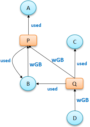
If or both inputs are modified, the entire execution must be re-run again. However, if only is modified, then the only part of the computation that will run differently is (i.e., will produce the same output , given the same input ). If is far more time-consuming than , it might suffice to run only , avoiding the expense of running again. Reducing the unneeded processing time is often critical if the execution is to be altered for a large number of modifications to input . This partial reproduction would be possible if, upon repeating the computation with its original inputs, the intermediate output produced by was saved in the container.
We use the embedded provenance graph to determine which part of the provenance graph need not be reprocessed again. Our algorithm is the same as Algorithm 2 in that we identify the primary processes of changed inputs, and from that determine the necessary and sufficient dependencies (i.e., getDeps function). This is the part of the graph that must be re-run. Nodes that are not in this dependency set are simply re-used from the container.
5 Summarizing Provenance Graphs
Provenance information generated by AV audit methods is fine-grained. A graph created from a complete set of generated provenance, using normal visualization structures such as tree or list representations, would be far too replete to be of real practical value. When viewed, this graph would present significant system-level detail that would inhibit a basic comprehension of the overall application workflow. For example, the intuitive workflow of Figure 1(a), consisting of 12 nodes and 13 edges, is represented fully as a dense provenance graph of 146 nodes and 321 edges. Figure 5(a) shows a part of this replete graph redrawn for visual clarity.
The definition of ‘intuitive’ is subjective. We consider two use cases with differing objectives in using the generated provenance graph: (i) a predominant process-view of the provenance graph sans the extraneous low-level system information generated due to auditing of common libraries and system executables; and (ii) a summarized graph that is (potentially) closer in appearance to an application workflow or prospective provenance as in Figure 1(a). In this section, we describe two formal methods for (i) and (ii). In (i), the key idea is to collapse or hide as much as possible common libraries and system executables, thus summarizing retrospective provenance; and, in (ii), the key idea is to summarize by finding groups of nodes and edges that may be related semantically to each other so as to potentially match with prospective provenance. We evaluate the first method based on total number of system information collapsed and second method based on available Unified Modeling language (UML) diagrams of our sample test programs. However, UML diagrams are not assumed as inputs to the summarization method and present as part of the sciunit.

5.1 Collapsing Retrospective Provenance
Given a directed graph , where is the set of vertices (in our graph, a vertex is of type “file” or of type “process”) and is the set of edges, we denote and as the sets of input and output edges of vertex . Respectively, , and . The direction of an edge characterizes the dependency of its vertices. For example, a process spawned by process is represented by the edge , and a file read by process is represented by the edge . The graph is collapsed based on the following two rules:
Rule 1.
Similarity. Two vertices and are called similar if and only if they share the same type and have the same input and output connection sets: , and .
The similarity rule groups multiple vertices into a single vertex if the vertices (i) have the same type and (ii) are connected by the same number and type of edges. Additionally, edges of similar vertices will be grouped into a single corresponding edge. Since the provenance graph follows W3C PROV-DM standard, each file is of type entity and each process is of type activity. When applied to our provenance graph, this rule groups different files and processes that are similar each other into the summary groups of files and processes (see Figure 5(a)).
Rule 2.
Packability. A vertex belongs to ’s if and only if vertex connects to and satisfies one of the following conditions:
-
[leftmargin=*,labelsep=5.8mm]
- •
Vertex is a file that has only one edge to process : and {}.
- •
Vertex is a process that has only one output edge to process : and {}.
- •
Vertex is a file that has only two edges—an output edge to process and an input edge from another process : and {}.
The packability rule identifies hubs in the provenance graph by packing files or processes that are connected by single edges to their parent nodes. It also packs files that are generated and consumed by a single process into their parent processes by producing a process-to-process edge.
When applied in sequence, the similarity and packability rules condense the detail-level of a graph while preserving its core workflow elements. Figure 5 (all process names and file names are simplified for brevity) illustrates how applying these two rules to a replete graph produces a graph summary that shows the primary processes in a workflow. Figure 5a presents the original replete provenance graph of one sub-task of the FIE workflow (the data processing steps “Calculate Violation” and “Calculate Heat Map” of Figure 1(a)). Applying the two summarization rules produces the graph in Figure 5(c).
We use an annotation method that assigns higher collapsibility to file nodes than process nodes, since an application workflow is typically defined by the primary processes that it runs. Figure 5(d) shows how the annotation “G_1”, which is a library dependency used both by “P_5” and “P_6”, is attached to the two process nodes that generated it. Thus, given a file with edges (), we replace this file with annotations.
Figure 6 shows the expanded view of node “P_R_27070” (“P_5” in Figure 5(b)). In Figure 6, similarity and packability rules group the nodes within the box into the single node “P_R_27070” (process 27070 runs a subprocess using file “21_calulate_violation_matrix.R” (“F_3” in Figure 5(b)) and write data to file “violation_data.Rds” (F_4 in Figure 5(b))). These nodes are application nodes and not system nodes. Here, “Process_G_5” (P_7 in Figure 5(b)), another concealing node, correctly hides all the dependencies of the R process calculating the violation matrix.

5.2 Summarizing Retrospective Provenance to Generate Prospective Provenance
The method in the previous section summarizes retrospective provenance by collapsing information. However, such summaries still differ from the conceptual view of the applications. For example, Figure 1(a), which is more familiar to users, is very different in view than Figure 5(d). Another equally important goal of summarization is to summarize retrospective provenance such that it (potentially) matches application workflow. In some situations, this application workflow may be available in the form of prospective provenance Dey et al. (2015). If available, summary methods can take advantage of this available information. In containers created of ad hoc applications, however, application workflows are rarely available. Therefore, we describe a summarization method that determines the lineage history of nodes and uses this information to summarize retrospective provenance.
Our method to summarize retrospective provenance is based on ideas described in SNAP (Summarization by Grouping Nodes on Attributes and Pairwise Relationships) Tian et al. (2008). SNAP is a non-statistical method for summarizing undirected and directed graph nodes and edges based on their respective types. In brief, it first groups nodes of the same type. It then recursively sub-divides to form smaller groups of nodes that still have have the same node type but also same relationship type with other groups. SNAP considers direct relationship types amongst group nodes and not relationship types due to ancestry of the nodes. Thus, grouping provided by SNAP can be further improved for provenance graphs by considering ancestral history of nodes while grouping. If ancestral relationships are considered, then, for a node, ancestors or descendants will not be grouped together since, by definition, the ancestral history of an ancestor and its descendent is different. Similarly, nodes in the same group will not share any relationship because then their ancestral history will be different.
To identify nodes with the same derivation history, first nodes of the same type are grouped, defined as
Definition 2 (Node Grouping).
Given a provenance graph , is a node-grouping such that
-
[leftmargin=2.3em,labelsep=4mm]
- (1)
or , and ,
- (2)
,
- (3)
and .
In particular, in (1), node grouping is over nodes of two types: activity nodes and entity nodes, in (2), the union of all node grouping is equal to the nodes in ; and, in (3), given a node grouping, groups are not overlapping, but distinct.
We now consider grouping by ancestry. For this, we identify the ancestors of a node as follows. For a given grouping , the ancestors of a node is the set . Type of edges is based on types used in W3C PROV standard where . Nodes that do not have an ancestor are assigned the start node as an ancestor, with a start label edge. Now, we define grouping nodes by ancestry.
Definition 3 (Ancestry grouping).
A grouping has the same ancestry if it satisfies the following:
-
[align=parleft,leftmargin=*,labelsep=3mm]
- (i)
Node Grouping Definition 2,
- (ii)
, if , then , .
Figure 7(a) shows the grouping of nodes due to SNAP, in which nodes with the same types and same ancestors are separated into different groups if their descendants are different, and due to ancestry grouping in Figure 7(b), in which nodes of the same type with same ancestors remain grouped.
Ancestry grouping, however, may still group system files and dependency information together with application-specific nodes. Consider the example in Figure 8. Suppose that we have a provenance graph on the left of Figure 8 that has three nodes of process ( and ), four nodes of file ( and ) and six edges (relationship ). The summary ancestry graph shown in center of Figure 8 dividing the original graph into two groups and , satisfies 3. (All nodes in every group have similar node types and associate with the same ancestry groups). However, from the conceptual point of view, file , a dependency used by other processes is different from other file nodes in , since this node is the only node that associates with all processes in group . In other words, has while other nodes in have .
To uniquely differentiate , we define ancestry-degree compatible grouping to summarize provenance graphs.
Definition 4 (Ancestry-degree grouping).
A grouping has the same ancestry-degree if it satisfies the following:
-
[align=parleft,leftmargin=*,labelsep=3mm]
- (i)
Ancestry grouping Definition 3,
- (ii)
, if , then , and , where and .

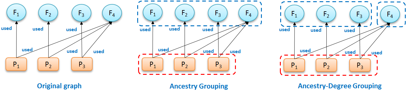
Based on this definition, the summary graph shown in Figure 8 (right) composed of three groups—, and —is ancestry-degree compatible because it is Ancestry-Grouping compatible and all the nodes in every group have the same number of output edges from/to other groups (all nodes in have one input edge from group , all nodes in group have two output edges: one to and one to ).
We now describe the summary algorithm, which, given a retrospective provenance graph, produces an ancestry-degree grouping. In this algorithm, we first divide the nodes into group with same node type and store them in a stack (Line 2). Next, for each group in the stack, we re-partition all groups in in stack by calling function divideGroup() with a list of vertices in (i.e., Lines 5–7). Function divideGroup() is called twice with different direction parameters, since it is applied on two different directions of edges (i.e., input or output). The main purpose of this function is to re-organize all the groups (i.e., ) that are relevant to by checking all the vertices and edges of vertices in group of stack (Lines 12 and 26). First, for each types of edges or relationships (in our context, there are three types of edge: ), it calculates the number of edges (or “degree”) from/to vertices in each group of to/from a vertex in (Lines 16–22). Second, it further divides these vertices in each group of by considering the degree of these vertices (i.e., the number of edges from/to vertices in group ). This means vertices that belong to the same group must have the same degree (Line 22). Third, we add all the new generated groups to if they have never been in (Lines 24–26), before the next consideration of other groups in . Finally, once all the groups in are considered, we obtain the summary graph by joining all the groups together (Lines 8–10).
Figure 9 presents an example of graph summarization. The left figure (i.e., Figure 9a) shows the work-flow of FIE City of Chicago (2017a) application drawn by users that describes the conceptual view of FIE application, while the right figure (i.e., Figure 9b) shows the provenance summary graph of FIE application after applying ancestry-degree grouping. As a general observation, these two graphs are fairly close to each other. The summary graph almost captures all the information about the application that users might need at the general view. There are some minor differences between them. For example, the two processes “Calculate heat map” and “Calculate violation” are clearly separate in the left figure while in the right figure they are grouped together. Similarly, the two groups of files “heat map data” and “Violation_dat.Rds” are separate in the left figure and grouped in the right. These groups of files and groups of processes are ancestry-degree compatible, and thus they are grouped in the right figure. While they are separate in the application workflow, ancestry-grouping is helpful in general. For instance, the ancestry-grouping grouped all data files into a single group at the top.

6 Experiments
The true usefulness of sciunits can only be measured by their adoption. Efficiency of creating sciunits can be a driving force in adopting the use of sciunits over traditional shared research objects. When an efficiently-versioned, easily-created sciunit is shared, along with an embedded, self-describing application workflow, we believe the probability for reuse will greatly increase. In this section, through two complex real-world workflows, we quantify the performance of containerizing and repeating sciunits, and the efficiency of reusing them utilizing integrated provenance visualizations. We implemented our Sciunit client in Python and C. The source code and documentation of Sciunit is available from https://sciunit.run Sci (2017).
Sciunit’s versioning tool was written in C++, using the block-based deduplication techniques proposed in Muthitacharoen et al. (2001) and Rabin (1981). sciunit’s provenance graph visualization was written in Python, using libraries from TensorBoard Tensorflow.org (2017). All sciunit client exec and repeat experiments, along with their baseline normal application runs, were conducted on a laptop with an Intel Core i7-4750HQ 2.0 GHz CPU, 16 GB of main memory, and a 1 TB SATA SSD (Solid state disk), running the Arch Linux 64-bit OS (at Chicago, Illinois, 60604, USA).
6.1 Use Cases
We consider two real-world use cases for experimental evaluation: (i) the Food Inspection Evaluation (FIE) City of Chicago (2017a) workflow, a computationally-intense use case that has been the running example in our paper, and (ii) Variable Infiltration Capacity (VIC) Billah et al. (2016) model, an I/O-intensive (Input/Output-intensive) data pre-processing pipeline for hydrology model.
The first use case is notable for its transparency in its rigorous inspection audits, owing to the influence of the Open Data movement within the City of Chicago. The second use case is a highly-relevant test bed for sciunits: the VIC model is very popular in the hydrology community, and its data preprocessing pipeline, which relies heavily on legacy code, is notoriously difficult to reassemble Billah et al. (2016).
Tables 1 and 2 describe the details of FIE and VIC in terms of source code file programming languages, number of source code and data files, number of program files required as dependencies, and total application sizes (both FIE and VIC have four sub-tasks, labeled 0, I, II, and III, which are described below). Figure 1(a) and Figure 10 show conceptual views of the application workflows for the two use cases.

We assume a sharing model, in which each step is conducted independently by one user, and subsequently shared with another user who builds upon or forks the shared workflow in the following step. Thus, the FIE workflow, for example, is broken down into the following sub-tasks, each encapsulated in a single application: (i) FIE_0, which calculates a heat map from downloaded inspection records; (ii) FIE_I, which processes the heat map to generate data model inputs; (iii) FIE_II, which applies a specific model and validates it; and (iv) FIE_III, which downloads the original inspection records and applies an end-to-end validation routine to the previous three sub-tasks. The download process of subtask iv is often the most time-consuming step.
| FIE_0 | FIE_I | FIE_II | FIE_III | |
| Source code languages | R, Bash | R, Bash | R, Bash | R, Bash |
| Source code files | 19 | 20 | 24 | 29 |
| Data files | 2 | 8 | 14 | 14 |
| Dependency files | 255 | 255 | 411 | 659 |
| Size of all files | 133.2 MB | 178.4 MB | 289.7 MB | 306.6 MB |
| Normal run time | 52.046 s | 238.833 s | 295.785 s | 7200 s |
| VIC_0 | VIC_I | VIC_II | VIC_III | |
| Source code languages | C, C++, Python, C shell script, Fortran | |||
| Source code files | 35 | 61 | 77 | 97 |
| Data files | 3689 | 6313 | 11,460 | 11,481 |
| Dependency files | 247 | 260 | 314 | 357 |
| Size of all files | 1.2 GB | 1.3 GB | 2.2 GB | 2.3 GB |
| Normal run time | 158.734 s | 306.069 s | 363.147 s | 377.29 s |
6.2 Creating Sciunits
Tables 1 and 2 present the baseline normal execution times for the sub-tasks of the two use cases. We note that each application encompasses substantial resources (in the form of code and data), has many external dependencies, and is also characterized by lengthy CPU-and-memory-intensive tasks. Additionally, the nature of FIE’s processing tasks differ significantly from those of VIC. FIE front-loads its input data sets into memory, and then utilizes machine-learning logic to process its data. VIC also runs many intricate calculations, but differs from FIE in that it interlaces file input and output operations regularly throughout its code. This difference is key in understanding that sciunits have minimal performance impact on most—but not all—types of applications.
Figure 11 compares the baseline normal execution time of each subtask with the time consumed by packaging the sub-task with the sciunit’s exec command, and with the time consumed by repeating the sub-task with the sciunit’s repeat command. Test results for the FIE_III and VIC_III sub-tasks were omitted due to significant amounts of network-dependent downloading operations. We note that the performance impact of auditing and repeating on FIE’s run times was negligible: auditing FIE with exec resulted in only a 3.6% time increase, and executing FIE with repeat added only a 1.3% increase to run time. Meanwhile, in FIE, the I/O access time is much less than CPU processing time. Also note that our tests were done on SSD offering much better performance than HDD (hard disk drive). The reasons explain why the overheads in these cases are negligible. Conversely, containerizing and repeating VIC with Sciunit nearly doubled the original application run times: as noted in the preceding paragraph, it was evident that using Sciunit with I/O-intensive (Input/Output-intensive) applications affected application performance significantly.
We obtain one further observation from these experiments by comparing each application exec time with its corresponding repeat time. Compared to application repeat increases, auditing increases were slightly higher. This difference can be understood by examining sciunit’s behavior during AV audit-time: auditing entails copying an application’s code and data into a sciunit container, but running the sciunit container with repeat, however, only redirects to these copied files, and therefore precludes the file copy time.

6.3 Repeatability Evaluation
To measure the exact repeat execution, we run all test cases presented in Tables 1 and 2 on many different environments such as Ubuntu, Arc Linux, CentOS 7, Fedora 26, RHEL 7 or Debian. The results are shown in Table 3.
As clearly shown in Table 3, these applications can be repeated successfully in all tested environments. We also applied Algorithm 1 to verify the provenance graph isomorphism between original runs and re-executions. The results are recorded in the column “Provenance graph isomorphism”. Since our isomorphism algorithm will finish when the first bijection is found, its performance is good even for large provenance graphs (e.g., it takes less than one second for handling with provenance graphs having up to 150 nodes and 320 edges).
| Repeatability | Execution Time (s) (Measured on | |||
| Our above Described Machine) | ||||
| Selected Applications | Re-execution (Tested on Ubuntu, Arc Linux, CentOS 7, Fedora 26, RHEL 7 or Debian) | Provenance Graph Isomorphism | Execution | Repeat |
| FIE_0 | Succeed | Matched | 52.046 | 53.954 |
| FIE_I | Succeed | Matched | 238.833 | 240.014 |
| FIE_II | Succeed | Matched | 295.785 | 297.681 |
| FIE_III | Succeed | Matched | 7,200 | 7,308.6 |
| VIC_0 | Succeed | Matched | 158.734 | 606.21 |
| VIC_I | Succeed | Matched | 306.069 | 1,140.5 |
| VIC_II | Succeed | Matched | 363.147 | 1,332.98 |
| VIC_III | Succeed | Matched | 377.29 | 1,384.89 |
6.4 Partial and Modified Repeat Execution
The main ideas of partial reproducibility are to reduce both execution time (only execute the necessary parts) and container size (not to include the data files or dependencies that will not be used). Therefore, we measure the partial reproducibility by the following criteria: (i) correctness; (ii) resource usability, and (iii) execution time.
Table 4 shows our evaluation on partial and modified reproducibility on the two selected use cases (i.e., FIE_III and VIC_III). In particular, we built the partial and modified containers on the originals of FIE_III and VIC_III. In FIE_III, we selected only the process ID that calculates the heat map from the downloaded file, and then built the sub-container (i.e., FIE_Par) using Algorithm 2. In particular, we note that in this experiment, Algorithm 2 used only direct descendants to build partial containers. A more general experiment using all descendants is in accompanying technical report Yuan et al. (2018). Meanwhile, the modified execution of FIE_III (i.e., FIE_Mod) was tested when we change the inputs (i.e., use new weather data file: “/tmp/weather_201801.Rds”) using the given command (see Section 3). Similarly, in VIC_III, we built the partial container (VIC_Par) with the process ID that only processes precipitation data. Table 4 shows the number of files and dependencies within the partial containers in comparison with those of original containers, as well as the differences in runtimes of repeat and original run. Values from row “# of files not used” denote that all files in the partial containers are touched when the application runs, indicating no extra file was included using Algorithm 2 in these partial containers. Meanwhile, row “Executable’” shows if partial and modified repeatability was successful.
| Original, Modified and Partial Executions of FIE_III | Original, Modified and Partial Executions of VIC_III | |||||
| Information | FIE_III | FIE_Mod | FIE_Par | VIC_III | VIC_Mod | VIC_Par |
| # of executable files | 29 | 29 | 19 | 97 | 97 | 35 |
| # of data files | 14 | 14 | 2 | 11,481 | 11,481 | 36 |
| # of dependencies | 659 | 659 | 255 | 357 | 357 | 247 |
| Executable | Succeed | Succeed | Succeed | Succeed | Succeed | Succeed |
| Execution time (s) | 7,200 | - | 52 | 377 | - | 159 |
| # of files not used | 0 | - | 0 | 0 | - | 0 |
6.5 Reusing Sciunits with Provenance Visualizations
Application virtualization has traditionally led to fine-grained provenance graphs that are often difficult to decipher. In this sub-section, we determine if our summarization rules produce a usable provenance graph that is closer to a theoretical, intuitive user application workflow. We focus this discussion on experiments for the FIE sub-tasks, but mention that experiment results for the VIC sub-tasks were similar.
To evaluate the effectiveness of summarization, we first considered three traditional, replete (i.e., fine-grained) provenance traces generated by Sciunit on auditing FIE_I, FIE_II, FIE_III (We did not consider FIE_0 in this analysis since its original replete graph was too small and simple to benefit measurably from summarization). We calculated the number of nodes (each a process or a file) and edges present in each replete graph. Next, we calculated the number of nodes present in the corresponding sciunit container provenance graphs. These graphs were summarized by using both the similarity and packability rules (i.e., collapsing retrospective provenance method) and ancestry-degree grouping method. Figure 12 depicts a comparison of these methods (i.e., original, collapsing retrospective provenance method and ancestry-degree grouping method).

Graph summarization reduced the number of file nodes, process nodes, and edges by averages of 88%, 41%, and 87% with graphs generated by collapsing retrospective provenance method and 90%, 91% and 93% with graphs generated by ancestry-degree grouping method.
We also measured the number of clicks needed to expand summarized graphs to replete graphs. For FIE_III, which had the largest graph, expanding any summarized node required a maximum of four user clicks to reach its replete view. Expanding all the nodes in this large graph took 45 clicks. This observation showed that graphs were summarized very well spatially and intuitively, yet still capable of allowing fully-detailed provenance examination with a modest amount of user interaction.
As seen in Figure 12, there are some differences between summary graphs from the collapsing retrospective provenance method and ancestry-degree grouping method. In general, applying the ancestry-degree grouping method is more efficient than collapsing retrospective provenance method in terms of number of objects. However, the graphs from collapsing retrospective provenance method are still clear and it is easy to understand the system detailed information. Indeed, the key differences between these two are the messages they deliver (see summary graphs in Figures 5 and 9). The summary graph from collapsing retrospective provenance method describes how an application be executed with its dependencies. Meanwhile, the one from ancestry-degree grouping method illustrates the conceptual view of an application. Therefore, we extend the new summarization method while keeping the old version and let users select between these methods according to which information they would prefer to examine.
7 Conclusions
Computational reproducibility Freire et al. (2012) is a formidable goal requiring advancements in policy Stodden et al. (2013), user perception Penny (2016), and reproducible practices and tools Stodden et al. (2014). As we embrace this goal within the sciences Malik (2017), we have encountered that computational provenance is the key to enhancing the experience of reproducible packages as created by the use of application virtualization. In this paper, we have outlined methods to create and store containers based on application virtualization and demonstrated an easy-to-use Git-like client, the Sciunit that enables reproducibility for a wide variety of use cases. We showed how embedded provenance can be used to reuse the sciunit and understand them by summarizing embedded provenance. The field of computational reproducibility is a moving target and there are emerging requirements to use provenance to address reproducibility within Jupyter notebooks Ma et al. (2017) , Matlab, distributed data-intensive programs, and parallel HPC applications, which we hope to address as part of future work.
Author Contributions
All authors contributed equally to the paper. Particularly, Z.Y., G.F., and T.M. designed and implemented Sciunit and provenance auditing. D.H.T.T. and T.M. developed algorithms for exact, partial, and modified repeat executions. D.H.T.T and G.F performed the experiments and analyzed the data. S.K. designed the prospective provenance summarization technique. T.M and D.H.T.T primarily wrote the paper.
Conflicts of Interest
The authors declare no conflict of interest.
References
- Miksa (2017) Miksa, T. Using ontologies for verification and validation of workflow-based experiments. Web Semant. Sci. Serv. Agents World Wide Web 2017, 43, 25–45.
- Belhajjame et al. (2015) Belhajjame, K.; Zhao, J.; Garijo, D.; Gamble, M.; Hettne, K.; Palma, R.; Mina, E.; Corcho, O.; Gómez-Pérez, J.M.; Bechhofer, S.; et al. Using a suite of ontologies for preserving workflow-centric research objects. Web Semant. Sci. Serv. Agents World Wide Web 2015, 32, 16–42.
- Stodden et al. (2014) Stodden, V.; Leisch, F.; Peng, R.D. (Eds.) Implementing Reproducible Research; CRC Press: Boca Raton, FL, USA, 2014; p. 448.
- Malik et al. (2014) Malik, T.; Pham, Q.; Foster, I.T. SOLE: Towards Descriptive and Interactive Publications. In Implementing Reproducible Research; Chapman & Hall/CRC, London, UK, 2014; Volume 33.
- Figshare.com (2017) Figshare.com. Figshare. Available online: https://figshare.com/ (accessed on 2 May 2017).
- Soiland-Reyes et al. (2014) Soiland-Reyes, S.; Gamble, M.; Haines, R. Research Object Bundle 1.0. 2014. Available online: https://researchobject.github.io/specifications/bundle/ (accessed on 2 May 2017).
- Chirigati et al. (2013) Chirigati, F.; Shasha, D.; Freire, J. ReproZip: Using Provenance to Support Computational Reproducibility. In Proceedings of the 5th USENIX Conference on Theory and Practice of Provenance (TaPP’13), Lombard, IL, USA, 2–3 April 2013; USENIX Association: Berkeley, CA, USA, 2013; p. 1.
- Janin et al. (2014) Janin, Y.; Vincent, C.; Duraffort, R. CARE, the Comprehensive Archiver for Reproducible Execution. In Proceedings of the 1st ACM SIGPLAN Workshop on Reproducible Research Methodologies and New Publication Models in Computer Engineering (TRUST), Edinburgh, UK, 9–11 June 2014; ACM: New York, NY, USA, 2014; pp. 1:1–1:7.
- Ton That et al. (2017) Ton That, D.H.; Fils, G.; Yuan, Z.; Malik, T. Sciunits: Reusable Research Objects. IEEE eScience 2017, Oct 24-27, 2017, Auckland, New Zealand, arXiv:1707.05731.
- De Roure (2013) De Roure, D. Towards Computational Research Objects. In Proceedings of the ACM Workshop on Digital Preservation of Research Methods and Artefacts, Indianapolis, IN, USA, 25 July 2013.
- Yale Roundtable (2010) The Yale Law School Roundtable on Data and Code Sharing. Reproducible Research 2010. Computing in Science Engineering 12, 8–13. Available online: http://ieeexplore.ieee.org/document/5562471/ (accessed on 5 March 2018).
- Bechhofer et al. (2013) Bechhofer, S.; Buchan, I.; De Roure, D.; Missier, P.; Ainsworth, J.; Bhagat, J.; Couch, P.; Cruickshank, D.; Delderfield, M.; Dunlop, I.; et al. Why linked data is not enough for scientists. Future Gener. Comput. Syst. 2013, 29, 599–611.
- Corcho et al. (2012) Corcho, O.; Garijo Verdejo, D.; Belhajjame, K.; Zhao, J.; Missier, P.; Newman, D.; Palma, R.; Bechhofer, S.; García Cuesta, E.; Gomez-Perez, J.M.; et al. Workflow-centric research objects: First class citizens in scholarly discourse. In Proceedings of Workshop on the Semantic Publishing, (SePublica 2012) 9 th Extended Semantic Web Conference Hersonissos, Crete, Greece, 28 May 2012.
- De Roure et al. (2011) De Roure, D.; Belhajjame, K.; Missier, P.; Gómez-Pérez, J.; others. Towards the Preservation of Scientific Workflows. In Proceedings of the 8th International Conference on Preservation of Digital Objects (iPRES), Singapore, 1–4 November 2011.
- Santana-Perez and Pérez-Hernández (2015) Santana-Perez, I.; Pérez-Hernández, M.S. Towards reproducibility in scientific workflows: An infrastructure-based approach. Sci. Program. 2015, 2015, 243180.
- RO- (2016) wf4ever/ro-manager. Available online: https://github.com/wf4ever/ro-manager (accessed on 2 May 2017).
- Standard OASIS (2013) Standard OASIS. Topology and Orchestration Specification for Cloud Applications Version 1.0; 2013. Available online: http://docs.oasis-open.org/tosca/TOSCA/v1.0/TOSCA-v1.0.html (accessed on 5 March 2018).
- Qasha et al. (2016) Qasha, R.; Cała, J.; Watson, P. A framework for scientific workflow reproducibility in the cloud. In Proceedings of the 12th International Conference on IEEE e-Science, Baltimore, MD, USA, 23–27 October 2016 .
- Guo and Engler (2011) Guo, P.J.; Engler, D. CDE: Using System Call Interposition to Automatically Create Portable Software Packages. In Proceedings of the USENIX Annual Technical Conference, Portland, OR, USA, June 15 - 17, 2011.
- Guo (2011) Guo, P.J. CDE: Run Any Linux Application On-demand without Installation. In Proceedings of the LISA’11: 25th Large Installation System Administration Conference, Boston, MA, USA, 4–9 December 2011.
- Pham et al. (2013) Pham, Q.; Malik, T.; Foster, I. Using Provenance for Repeatability. In Proceedings of the TaPP, Lombard, Illinois, USA, April 02 - 03, 2013.
- Thain et al. (2015) Thain, D.; Ivie, P.; Meng, H. Techniques for Preserving Scientific Software Executions: Preserve the Mess or Encourage Cleanliness? In Proceedings of the 12th International Conference on Digital Preservation (iPRES 2015), Chapel Hill, NC, USA, 2–6 November 2015.
- Docker (2017) Docker. 2017. Available online: https://www.docker.com/ (accessed 2 May 2017).
- Vagrant (2017) Vagrant. 2017. Available online: https://www.vagrantup.com/ (accessed on 2 May 2017).
- Meng et al. (2015) Meng, H.; Kommineni, R.; Pham, Q.; Gardner, R.; Malik, T.; Thain, D. An invariant framework for conducting reproducible computational science. J. Comput. Sci. 2015, 9, 137–142.
- Muthitacharoen et al. (2001) Muthitacharoen, A.; Chen, B.; Mazières, D. A Low-bandwidth Network File System. In ACM SIGOPS Operating Systems Review; ACM, New York, NY, USA, Dec. 2001; Volume 35, pp. 174–187.
- Murta et al. (2014) Murta, L.; Braganholo, V.; Chirigati, F.; Koop, D.; Freire, J. noWorkflow: Capturing and analyzing provenance of scripts. In International Provenance and Annotation Workshop; Springer: Cologne, Germay, 2014, pp. 71–83.
- Muniswamy-Reddy et al. (2006) Muniswamy-Reddy, K.K.; Holland, D.A.; Braun, U.; Seltzer, M.I. Provenance-aware storage systems. In Proceedings of the General Track: USENIX Annual Technical Conference, Boston, MA, USA, May 30 - June 03, 2006, pp. 43–56.
- Gehani and Tariq (2012) Gehani, A.; Tariq, D. SPADE: Support for provenance auditing in distributed environments. In Proceedings of the 13th International Middleware Conference, Montreal, QC, Canada, 3–7 December 2012; Springer: New York, NY, USA, 2012; pp. 101–120.
- Pham et al. (2015) Pham, Q.; Malik, T.; Glavic, B.; Foster, I. LDV: Light-weight database virtualization. In Proceedings of the 2015 IEEE 31st International Conference on Data Engineering (ICDE), Seoul, Korea, 13–17 April 2015 .
- Pham (2014) Pham, Q. A Framework for Reproducible Computational Research. Ph.D. Thesis, Department of Computer Science, University of Chicago, Chicago, IL, USA, 2014.
- Dey et al. (2015) Dey, S.; Belhajjame, K.; Koop, D.; Raul, M.; Ludäscher, B. Linking Prospective and Retrospective Provenance in Scripts. In Proceedings of the 7th USENIX Conference on Theory and Practice of Provenance (TaPP’15), Edinburgh, Scotland, 8–9 July 2015; USENIX Association: Berkeley, CA, USA, 2015; p. 11.
- McPhillips et al. (2015) McPhillips, T.M.; Song, T.; Kolisnik, T.; Aulenbach, S.; Belhajjame, K.; Bocinsky, K.; Cao, Y.; Chirigati, F.; Dey, S.C.; Freire, J.; et al. YesWorkflow: A User-Oriented, Language-Independent Tool for Recovering Workflow Information from Scripts. CoRR 2015. Volume 10, pp. 298–313.
- Macko et al. (2013) Macko, P.; Margo, D.; Seltzer, M. Local clustering in provenance graphs. In Proceedings of the 22nd ACM international conference on Information & Knowledge Management (CIKM), San Francisco, CA, USA, 27 October–1 November 2013; ACM: New York, NY, USA, 2013.
- Cohen et al. (2006) Cohen, S.; Cohen-Boulakia, S.; Davidson, S. Towards a model of provenance and user views in scientific workflows. In Data Integration in the Life Sciences; Springer: Berlin/Heidelberg, Germany, 2006.
- El-Jaick et al. (2014) El-Jaick, D.; Mattoso, M.; Lima, A.A.B. SGProv: Summarization Mechanism for Multiple Provenance Graphs. J. Inf. Data Manag. 2014, 5, 16–27.
- Sci (2017) The Sciunit. 2017. Available online: https://sciunit.run/ (accessed on 10 September 2017).
- City of Chicago (2017a) City of Chicago. Food Inspection Evaluation. 2017. Available online: https://chicago.github.io/food-inspections-evaluation/ (accessed on 5 May 2017).
- City of Chicago (2017b) City of Chicago. Chicago Data Portal. 2017. Available online: https://data.cityofchicago.org/ (accessed on 7 May 2017).
- City of Chicago (2016) City of Chicago. Food Inspection Evaluation Predictions-Source Code. 2016. Available online: https://github.com/Chicago/food-inspections-evaluation (accessed on 7 May 2017).
- City of Chicago (2017) City of Chicago. Food Inspection Evaluation. 2017. Available online: https://chicago.github.io/food-inspections-evaluation/predictions/ (accessed on 5 May 2017).
- Goecks et al. (2010) Goecks, J.; Nekrutenko, A.; Taylor, J. Galaxy: A comprehensive approach for supporting accessible, reproducible, and transparent computational research in the life sciences. Genome Biol. 2010, 11, R86.
- Zhao et al. (2007) Zhao, Y.; Hategan, M.; Clifford, B.; Foster, I.; von Laszewski, G.; Nefedova, V.; Raicu, I.; Stef-Praun, T.; Wilde, M. Swift: Fast, Reliable, Loosely Coupled Parallel Computation. In Proceedings of the IEEE Congress on Services, Salt Lake City, UT, USA, 9–13 July 2007; pp. 199–206.
- Altintas et al. (2006) Altintas, I.; Barney, O.; Jaeger-Frank, E. Provenance Collection Support in the Kepler Scientific Workflow System. In International Provenance and Annotation Workshop IPAW; Springer, Berlin/Heidelberg, Germany, 2006.
- Hydroshare.com (2017) Hydroshare. 2017. Available online: https://www.hydroshare.org/ (accessed on 2 May 2017).
- McKay (1981) McKay, B.D. Practical Graph Isomorphism. Congres. Numer. 1981, 30, 45–87.
- McKay (2017) McKay, B.D. The Page Nauty. 2017. Available online: http://users.cecs.anu.edu.au/~bdm/nauty/ (accessed on 10 September 2017).
- Wolfram (2017) Wolfram. Find Graph Isomorphism. 2017. Available online: http://reference.wolfram.com/language/ref/FindGraphIsomorphism.html (accessed on 10 September 2017).
- Tian et al. (2008) Tian, Y.; Hankins, R.A.; Patel, J.M. Efficient Aggregation for Graph Summarization. In Proceedings of the 2008 ACM SIGMOD International Conference on Management of Data (SIGMOD ’08), Vancouver, BC, Canada, 9–12 June 2008; ACM: New York, NY, USA, 2008; pp. 567–580.
- Billah et al. (2016) Billah, M.M.; Goodall, J.L.; Narayan, U.; Essawy, B.T.; Lakshmi, V.; Rajasekar, A.; Moore, R.W. Using a data grid to automate data preparation pipelines required for regional-scale hydrologic modeling. Environ. Model. Softw. 2016, 78, 31–39.
- Rabin (1981) Rabin, M.O. Fingerprinting by Random Polynomials; Center for Research in Computing Technology, Aiken Computation Lab., Harvard University, Cambridge, MA, USA 1981.
- Tensorflow.org (2017) Tensorflow. 2017. Available online: https://www.tensorflow.org/ (accessed on 2 May 2017).
- Freire et al. (2012) Freire, J.; Bonnet, P.; Shasha, D. Computational Reproducibility: State-of-the-art, Challenges, and Database Research Opportunities. In Proceedings of the 2012 ACM SIGMOD International Conference on Management of Data, Scottsdale, AZ, USA, 20–24 May 2012.
- Stodden et al. (2013) Stodden, V.; Guo, P.; Ma, Z. Toward Reproducible Computational Research: An Empirical Analysis of Data and Code Policy Adoption by Journals. PLoS ONE 2013, 8, e67111.
- Penny (2016) Penny, D. Nature Reproducibility Survey. Available online: https://figshare.com/articles/Nature_Reproducibility_survey/3394951 May 2016. (accessed on 5 March 2018).
- Malik (2017) Malik, T. GeotrustHub. Available online: https://geotrusthub.org/ (accessed on 10 September 2017).
- Ma et al. (2017) Ma, X.; Beaulieu, S.E.; Fu, L.; Fox, P.; Di Stefano, M.; West, P., Documenting Provenance for Reproducible Marine Ecosystem Assessment in Open Science. In Oceanographic and Marine Cross-Domain Data Management for Sustainable Development; Diviacco, P., Leadbetter, A., Glaves, H., Eds.; IGI Global, Hershey, PA, USA; 2017; Chapter 5, pp. 100–126.
- Malik et al. (2013) Malik, T.; Gehani, A.; Tariq, D.; Zaffar, F. Sketching distributed data provenance. Data Provenance and Data Management in eScience, Springer, Berlin, Heidelberg, Germany, 2013; pp. 85–107.
- Yuan et al. (2018) Yuan, Z.; Ton That, D. H.; Kothari, S.; Fils, G; Malik, T.. Sciunit Technical report. Available online: https://sciunit.run/papers/DBGroup-TechReport-MDPI2018.pdf (accessed on 7 March 2018).