Pulsing dynamics in randomly wired
glider cellular automataThanks: edward.coxon@act.gov.au

Andrew Wuensche ^†^†thanks: andy@ddlab.org, http://www.ddlab.org Discrete Dynamics Lab. Affiliation: Edward Coxon Dept. of Anaethesia and Pain Medicine, Affiliation: The Canberra Hospital, ACT, Australia.

Abstract

Sustained rhythmic oscillations, pulsing dynamics, emerge spontaneously when the local connection scheme is randomised in 3-value cellular automata that feature“glider” dynamics. Time-plots of pulsing measures maintain a distinct waveform for each glider rule, and scatter plots of entropy/density and the density return-map show unique signatures, which have the characteristics of chaotic strange attractors. We present case studies, possible mechanisms, and implications for oscillatory networks in biology.

keywords: cellular automata, glider dynamics, random wiring, pulsing, bio-oscillations, emergence, chaos, complexity, strange attractor, heartbeat, sympathetic centre, central pattern generator

1 Introduction

Arguably the most interesting manifestation of cellular automata dynamics is the emergence of mobile (and stable) configurations known as particles or gliders which interact by collisions, possibly making compound emergent structures such as glider-guns in an open ended hierarchy — components which can sometimes be rearranged to achieve universal computation[2, 13]. Glider dynamics arise within rare “complex” rules, which also include dynamics apart from gliders, for example, dynamic patches, blinkers, or mobile boundaries between domains. Otherwise the dynamics and rule types, broadly speaking, are either “ordered” or “disordered” judged by subjective impressions of space-time patterns, but also by objective measures such as input-entropy and its variability[32], basin of attraction topology[31], and Derrida plots[10, 38]. By any evaluation, disorder comprises the vast majority of large rule-spaces.

We pose the question: while preserving a homogeneous rule, what kind of dynamics would result if the regular local neighborhood connections (the wiring) of classical CA are randomised? — an experiment readily implemented in DDLab[38, 39], with its functionality for toggling between regular and random wiring on-the-fly, and where random wiring can be fully random or confined in a local zone, or even re-randomised at each time-step.

The results of these “random wiring” experiments reveal a novel and remarkable phenomenon — for 3-value, k-totalistic, “glider” CA rules, sustained rhythmic oscillations, pulsing behaviour, is the inevitable outcome. The pulsing is obvious to the subjective eye when observing space-time patterns, but is also characterised by objective measures: the density of each value across the network, and the collective input-entropy. Time-plots of pulsing measures for each glider rule maintain a particular wavelength ( $wl$ ), wave-height ( $wh$ , twice amplitude), and waveform (its shape or phase), and scatter plots of entropy/density[32] and the density return-map[38] show distinct signatures, which have the characteristics of chaotic strange attractors. We will use the term “waveform” to sum up these pulsing measures, and the “CA pulsing model” for the system itself. We demonstrate pulsing when the wiring is fully (and sometimes partly) randomised. Pulsing is robust to re-randomised wiring at each time-step, to noise, to boundary conditions, and to asynchronous or sequential updating. When random wiring is confined in a relatively small local zone, spiral density waves, reminiscent of reaction-diffusion, can emerge in a large enough system, so local pulsing is still present (figure 14) as waves sweep over local areas of the lattice.

Experiment shows that pulsing does not occur for ordered or disordered rules, or for complex rules that do not feature well defined gliders. Pulsing is not discernible for glider rules in binary CA, such as the 1D rule 110, the 2D Game-of-Life[13], or other binary rules that support gliders and glider-guns[14, 15, 16, 27]. We can find large samples of complex rules by classifying rule-space automatically according to the variability of input-entropy[32, 33, 39]. Within these samples a significant proportion are glider rules.

We focus on 3-value k-totalistic¹¹ 1 Non-totalistic 3-value glider rules and 4-value k-totalistic glider rules, which are harder to find, will be examined in due course. glider CA on a 2D hexagonal lattice (and some extension to 3D) with neighbourhoods²² 2 The CA pulsing model has also been demonstrated for neighbourhoods of 4 and 5. of 6 or 7, including two well known CA rules that have been studied in depth, the Beehive rule[3, 33, 34], and the Spiral rule[4, 35, 36]. The CA pulsing model is interesting in its own right, and may also help to understanding and model oscillatory networks in biology. We address the questions that arise about possible mechanisms, thought this paper is primarily concerned with presenting and documenting the phenomena.

The paper is organised as follows: Section 2 describes CA and random wiring. Section 3 defines 3-value k-totalistic rules. Section 4 defines input-frequency and input-entropy. Section 5 presents detailed pulsing case studies, including different aspects of the waveform. Sections 7 — 9 examine the consequences of freeing one wire from localised neighborhoods, including 3D systems. In sections 10 — 12 we discuss reaction-diffusion, asynchronous and noisy updating, and possible pulsing mechanisms. In sections 13 and 14 we discuss the implications for bio-oscillations, ubiquitous at many time/size scales in biology, and for modeling oscillatory behaviour in mammalian tissue such as the heart and central nervous system.

2 CA and random wiring

$k$ =6

$k$ =7

Figure 1: The (pseudo)-neighborhood template for hexagonal 2D CA,

k

=6 and

k

=7, with template cells numbered as in DDLab (for 3D see figure 16)

(a)

(b)

(c)

Figure 2: A hexagonal lattice 10

\times

10 showing

k

random cells (green) wired to the target cell, (a) and (b) via a pseudo-neighborhood template (yellow and red), and (c) directly. (a) For

k

=6 the target cell is not included in its neighborhood. (b) For

k

=7 the target cell (red) is included. For CA the actual neighborhood and pseudo-neighborhood are identical. (c) For k-totalistic rules and random wiring, strictly speaking, a pseudo-neighborhood template is not required.

In classical CA, the pattern on the lattice updates (in discrete time-steps) as each (target) cell synchronously³³ 3 Asynchronous and noisy updating is discussed in section 11. updates its value according to the values in its local neighborhood template. In the general case the updating function is a lookup-table (rule-table) of all $v^{k}$ possible neighborhood patterns, were $v$ is the value-range and $k$ is the neighborhood size.

In this paper we focus mainly on 2D CA on a hexagonal lattice, with a local neighborhood “template” of $k$ =6 and $k$ =7 (figures 1 and 2), and also 3D in section 9. Boundary conditions are periodic (toroidal for 2D) — effectively no boundaries, but this is not significant in the CA pulsing model. The $k$ =6 template is shown in yellow surrounding the target cell, whereas the $k$ =7 template includes the (red) target cell. Template cell numbers permit a complete non-totalistic rule-table to be assigned according to DDLab’s convention[38].

To implement “random wiring”, as in Kauffman’s “Random Boolean Networks” [21], for each target cell, we take $k$ cells at random in the lattice and “wire” them to distinct cells in the pseudo-neighborhood template — “pseudo” because the actual template values are replaced by the values of the random cells. Each target cell is assigned its own random wiring. The random wiring can be biased in many ways in DDLab[38], one of which is to confine random wiring within a local zone of arbitrary size (section 7). One or more wires can be “freed” from the zone, or from a CA neighborhood. Using DDLab, a single key press enables switching between CA and any type of preset random wiring, or between stable random wiring and re-randomising the wiring at each time-step (within preset parameters) as in Derrida’s annealed model[10].

The (pseudo)-neighborhood template allows a full rule-table, including isotropic rules, in various geometries and dimensions. For k-totalistic rules, however, though each incoming wire must connect to a distinct template cell, which one is irrelevant.

3 k-totalistic rules

v3k6 kcodeSize=28
(hex) 0a0282816a0264
(kcode-table:2-0)
0022000220022001122200021210
vfreq=11+4+13=28
  27: 6 0 0  -> 0
  26: 5 1 0  -> 0
  25: 5 0 1  -> 2
  24: 4 2 0  -> 2
  23: 4 1 1  -> 0
  22: 4 0 2  -> 0
  21: 3 3 0  -> 0
  20: 3 2 1  -> 2
  19: 3 1 2  -> 2
  18: 3 0 3  -> 0
  17: 2 4 0  -> 0
  16: 2 3 1  -> 2
  15: 2 2 2  -> 2
  14: 2 1 3  -> 0
  13: 2 0 4  -> 0
  12: 1 5 0  -> 1
  11: 1 4 1  -> 1
  10: 1 3 2  -> 2
   9: 1 2 3  -> 2
   8: 1 1 4  -> 2
   7: 1 0 5  -> 0
   6: 0 6 0  -> 0
   5: 0 5 1  -> 0
   4: 0 4 2  -> 2
   3: 0 3 3  -> 1
   2: 0 2 4  -> 2
   1: 0 1 5  -> 1
   0: 0 0 6  -> 0
   \  - - -     \
    \ 2 1 0    kcode (outputs)
     \  \
      \  totals of 2s, 1s, 0s
       \  in the neighborhood
        \
       kcode index

(a) $v3k6$ kcode
Beehive rule[33]

v3k7 kcodeSize=36
(hex) 020609a2982a68aa64
(kcode-table:2-0)
000200120021220221200222122022221210
vfreq=18+6+12=36
  35: 7 0 0  -> 0
  34: 6 1 0  -> 0
  33: 6 0 1  -> 0
  32: 5 2 0  -> 2
  31: 5 1 1  -> 0
  30: 5 0 2  -> 0
  29: 4 3 0  -> 1
  28: 4 2 1  -> 2
  27: 4 1 2  -> 0
  26: 4 0 3  -> 0
  25: 3 4 0  -> 2
  24: 3 3 1  -> 1
  23: 3 2 2  -> 2
  22: 3 1 3  -> 2
  21: 3 0 4  -> 0
  20: 2 5 0  -> 2
  19: 2 4 1  -> 2
  18: 2 3 2  -> 1
  17: 2 2 3  -> 2
  16: 2 1 4  -> 0
  15: 2 0 5  -> 0
  14: 1 6 0  -> 2
  13: 1 5 1  -> 2
  12: 1 4 2  -> 2
  11: 1 3 3  -> 1
  10: 1 2 4  -> 2
   9: 1 1 5  -> 2
   8: 1 0 6  -> 0
   7: 0 7 0  -> 2
   6: 0 6 1  -> 2
   5: 0 5 2  -> 2
   4: 0 4 3  -> 2
   3: 0 3 4  -> 1
   2: 0 2 5  -> 2
   1: 0 1 6  -> 1
   0: 0 0 7  -> 0

(b) $v3k7$ kcode
Spiral rule[35]

Table 1: The kcode is a rule-table listing the output for every combination of value totals in the neighborhood. For a system with 3 values (colors) the list is ordered by the number of 2s, 1s, 0s, taken as a decimal number. The kcode is then a string listing each output in descending order, from left to right, which can a be converted to hexadecimal for compactness. In DDLab these methods are implemented automatically, for

v\leq 8

and

k\leq 27

. These examples show the kcode for the Beehive rule and Spiral rule — their pulsing dynamics are examined below.

We focus on 3-value k-totalistic rules for the following reasons: their rule-tables are relatively short and thus tractable for displaying the input-frequency histogram and its entropy (input-entropy); the dynamics are isotropic so closer to nature; and the availability of samples of glider rules. At present gilder rules are found by looking at complex rules — examining their space-time dynamics by eye, though pulsing itself could provide the basis for an automatic search (section 12). Complex rules themselves are found automatically by classifying rule-space by the variability of input-entropy method[32, 33, 38].

In k-totalistic rules the output depends on just the combination of totals, or frequencies, of the values in the neighborhood, making k-totalistic rules a special case of isotropic rules — the same output for neighborhood rotation or reflection. Each combination of totals make up the rule-table (kcode), which has $S=(v+k-1)!/(k!\times(v-1)!)$ entries. Figure 1 explains the rule system for $v3k6$ where $S$ =28, and for $v3k7$ where $S$ =36, taking as examples the Beehive rule[33] and the Spiral rule[35]. The size of k-totalistic rule-space is $v^{S}$ .

Refer to caption — Figure 3: Dynamic graphics in DDLab show up pulsing in the $v3k6$ Beehive rule[33] (hex 0a0282816a0264) on a 100 $\times$ 100 hexagonal lattice with fully random wiring. The period varies between 7 and 8 time-steps.
(top) A typical sequence of the space-time patterns displaying pulsing densities, and related input-histograms, repeating on the 8th time-step. The horizontal bars represent the lookup-frequency of 28 neighborhoods, as in figure 1(a). Below (arrows show time’s direction): (a) The input-histogram shown scrolling with time (z-axis). (b) Plotting the input-histograms values (x-axis) for successive time-steps (y-axis). (c) Input-entropy values (x-axis) plotted for successive time-steps (y-axis).

4 The input-frequency and input-entropy

The input-frequency histogram tracks how frequently the different entries in a rule-table are actually looked up. This is usually averaged over a moving window of $w$ time-steps[32] to classify rules by the variability of input-entropy, but to track pulsing dynamics we take the measures over each time-step. The input-entropy is the Shannon entropy $H$ of this input-frequency histogram. $H$ , at time-step $t$ , for one time-step ( $w$ =1), is given by $H^{t}=-\sum_{i=0}^{S-1}\left({Q_{i}^{t}}/{n}\times log_{2}\left({Q_{i}^{t}}/{n}\right)\right)$ , where $Q_{i}^{t}$ is the lookup-frequency of neighborhood $i$ at time $t$ . $S$ is the rule-table size, and $n$ is the network size. The normalised Shannon entropy $H_{N}$ is a value between 0 and 1, $H_{N}=H^{t}/log_{2}n$ , which measures the heterogeneity of the histogram — henceforth “entropy” will refer to $H_{N}$ . Figure 3 shows how space-time patterns, their input-frequency (histogram), and the input-entropy measures are tracked by dynamic graphics in DDLab to show up pulsing, taking the $v3k6$ Beehive rule[33] as an example.

5 Pulsing case studies

We present six case studies of the CA pulsing model, based on glider rule samples assembled previously[38], three for $k$ =6 (figures 5-7), and three for $k$ =7, (figures 8-10), selected for a variety of waveform profiles. Surprisingly, wave-lengths ( $wl$ ) are very diverse, with average $wl$ varying between 6 and 82 time-steps. Two well documented rules are included, the $v3k6$ Beehive rule[3, 33, 34], and the $v3k7$ Spiral rule[35, 4, 36].

Each case study examines pulsing dynamics on a 2D 100 $\times$ 100 hexagonal lattice. Random wiring is unconstrained (giving the “RW-waveform”) where the $k$ inputs to each cell are independently assigned at random without bias. This makes the 2d geometry irrelevant — it is retained for convenience.

The results are displayed graphically as follows:

•

(a) A typical snapshot before the wiring was randomised, of the CA with its emergent gliders, with 10 time-step green trails.
•

(b, c) Two snapshots after the wiring was randomised, showing the now disordered pattern (b) at its minimum and (c) maximum density of non-zero values (2=black, 1=red, 0=white).
•

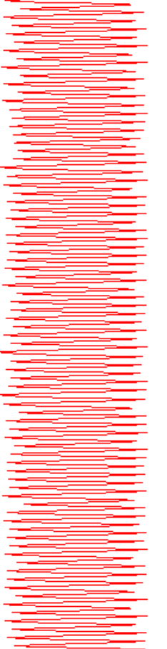
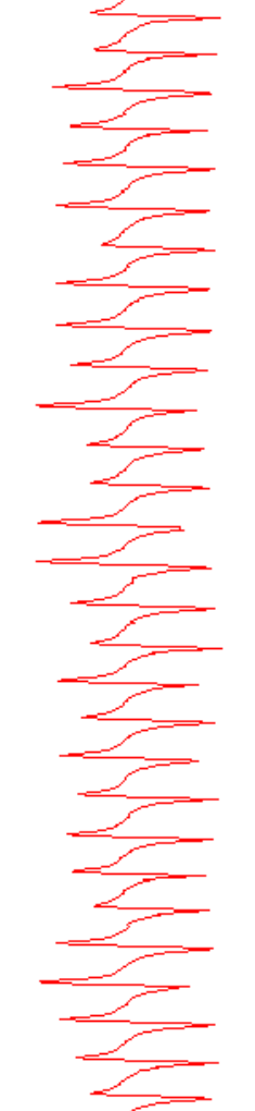
(d, e) Space-time patterns showing evidence of pulsing, with cells colored according to lookup instead of value, following the histogram colors in figure 3. (d) 2D space-time patterns scrolling diagonally, with the latest time-step at the front, leaving a trail of time-steps behind. (e) A stretch of the space-times pattern transformed to 1D, scrolling vertically, with the present moment at the bottom, leaving a trail of time-steps behind.
•

(f1) The input-entropy plotted for each time-step, showing the pulsing waveform. (f2) A stretched or magnified version of this plot, noting the wavelength $wl$ and wave-height $wh$ .
•

(g) The entropy-density scatter plot — input-entropy (x-axis) against the non-zero density (y-axis), plotted as blue dots, for about 33000 time-steps.
•

(h) The density return-map scatter plot — the density of each value at $t_{0}$ (x-axis) against its density at $t_{1}$ , plotted as colored dots (2=black, 1=red, 0=green), for about 33000 time-steps.

Case study experiments (confirmed for many other glider rules) give the following general results: Any random initial state, (within reason⁴⁴ 4 Initial states with some of the 3-values missing, or with very low/high density may not converge on the waveform.) will initiate a transient that rapidly converges on the waveform, which is impervious to reasonable noise. With fully random wiring (without bias), changing the actual wiring makes no difference to the waveform, neither does re-randomising at each time-step. The scatter plots, both input-entropy and the density return-map, show unique signatures, which have the characteristics of chaotic strange attractors in the context of deterministic discrete dynamical systems — sensitivity to initial conditions evolving towards a compact global attracting set, local instability but globally stability. Varying the network size also preserves the waveform — the signatures are diffused for small sizes, becoming more focused as the size of the network increases (figure 4), and this would continue towards infinity. Reducing the network size, however, increases the probability of reaching a uniform value attractor, such as all zeros, where the system would stop.

The “RW-waveform” results of these case studies will serve as a base of comparison with the other wiring biases investigated: CA with freed wires, localised random wiring (and with freed wires), and the equivalent in 3D.

6 Freeing one wire from CA neighborhoods

If one wire is released from each neighborhood in the 2D CA, and freely connected anywhere in the lattice, glider dynamics is destroyed and we may begin to see pulsing. Freeing one wire results in significant pulsing in all three $k$ =6 rules in our case study (figure 11), and is also probable in other $k$ =6 glider rules. For $k$ =7, pulsing is less probable because a smaller proportion of the neighbrhood is randomised — only one rule from the case study gave distinct pulsing (figure 12). If two wires are freed, pulsing is highly probable for both $k$ =6 and $k$ =7, and with more free wires pulsing properties approach the RW-waveform. The waveform is unaffected by re-randomising at each time-step.

7 Localised random wiring

Figure 13: (Left) Random wiring confined within 20

\times

20 local zones within a 300

\times

300 hexagonal lattice (

f=

20/300

\approx

0.066), (Right) shows a detail.

How does the dynamics play out if random wiring is confined within a local zone relative to each target cell? — as in figure 13, which makes the 2D geometry of the lattice significant, whereas with fully random wiring the geometry loses significance. Experiment shows that as the local zone diameter $d$ is reduced relative to the network diameter $D$ — the reach of random wiring — overall pulsing, though still apparent, turns into patchy waves of density. At some threshold (of the fraction $f$ = $d/D$ ) the stability and shape of the waveform will start to deform relative to the RW-waveform, and eventually break down, a process that could be interpreted as a type of phase transition, though a proper description will require further research and analysis. Preliminary results show that the threshold $f_{T}$ is independent of network size, but varies according to the rule. For $v3k7$ rules in figures 8, 9, 10, $f_{T}\approx$ 0.08, 0.05, 0.24, respectively. Above this relatively low threshold the pulsing waveform is robust.

As the local zone is further reduced, spiral density waves, reminiscent of reaction-diffusion, can emerge in a large enough system (figure 14) with local pulsing as waves sweep across a local area. Re-randomising the wiring at each time-step makes no significant difference to the general behaviour.

8 Freeing one wire from localised neighborhoods

Freeing just one wire from the 20 $\times$ 20 localised random zone in section 7, allowing it to connect anywhere, restores pulsing behaviour, but with a patchy distribution of values. Experiment confirms this applies to all the rules in the pulsing case studies in section 5 –10. The waveforms are still recognisable when compared to the RW-waveforms, including the entropy-density and density return-map scatter plot signatures. For example, the $v3k7$ “g3” rule waveform (figure 15) can be compared with its RW-waveform in figure 9.

9 3D systems

(a)

(b)

(c)

Figure 16: (a) 3D neighborhoods,

k

=6 and

k

=7. (b) 3D 45

\times

\times

45 lattice with unrestrained random wiring. (c) Random wiring restrained in a 5

\times

\times

5 local zone, but with one wire freed.

3D $k$ =6 and $k$ =7 CA (figure 16) were implemented in a 3D cubic lattice 45 $\times$ 45 $\times$ 45 with periodic boundaries. We found that all the rules in the case study (section 5) exhibit 3D glider behaviour, and fully random wiring gave the same pulsing waveforms as 2D (figure 17 Top) — not surprisingly because the shape of the neighborhood is not significant for an isotropic rule.

When random wiring is confined within 5 $\times$ 5 $\times$ 5 local zones, pulsing is still evident with strange attractor signatures deformed (figure 18). However, when one wire is freed the signatures revert closer to RW-waveforms (figure 17 Bottom).

10 k-totalistic rules as reaction-diffusion systems

An explanation of glider dynamics in k-totalistic rules can be based on Adamatsky’s reinterpretation of the $k$ =6 Beehive rule[3], and the $k$ =7 Spiral rule[35, 4], as discrete models of reaction-diffusion systems with inhibitor/activator reagents in a chemical medium. The three CA values are seen as: A=1 (Activator), I=2 (Inhibitor), and S=0 (Substrate). The three reagents perform a sort of non-linear feedback dance, suppressing and catalysing each other at critical concentrations. The analysis accounts for the movement of a glider’s head and following tail, but could also apply to the randomly wired system seen as a neural network with three states: 1=(Activator, Firing), 2=(Refractory), 0=(Ready to Fire). When wiring is randomized, it seems that feedback becomes distributed, giving global pulsing instead of driving a glider.

In glider CA, gliders and their interactions quickly dominate the dynamics, and thus the frequency of neighborhood lookup in the rule-table. The neighborhoods responsible for the background “domain” are the most frequent, followed by neighborhoods that drive gliders, other (stable) structures, and those invloved in collisions. The remaining neighborhoods rarely appear in an evolved system and can be regarded as wild-cards in the rule-table — mutations of these have little or no effect[34, 36].

This is captured by the lookup-frequency histograms (figure 19) for the Beehive and Spiral rules[33, 35], averaged over 100 time-steps, where the CA histogram highlights the background domain and glider dynamics, and the wild-cards by gaps or reduced values. The histogram for random wiring has a less pronounced distribution, but there is a significant correlation with the CA histogram, showing that the feedback between the three values is at play globally. Histograms for the other rules studied confirm these results.

11 Asynchronous and noisy updating

In the results so far, updating the next time-step has been deterministic, and synchronous (in parallel) across the lattice — but what would be the effects of noise and asynchronicity? DDLab has a suite of options to introduce either or both on-the-fly[38]. Two types of noise are implemented where each cell updates with a given probability at each time-step — otherwise, in one alternative the cell stays the same, and in the other its value is assigned randomly. For asynchronicity, the most flexible method is “partial order” updating where a subset of cells update (synchronously or sequentially), followed by the next subset — then the “state” is the configuration after each updated subset. Lower and upper limits predefine the size of each subset between 1 and network size $n$ . At each time-step, a random size is set between these limits, and scattered randomly to positions in the network — only those are updated. In sequential updating, each cell is updated in turn in some arbitrary order — then the “state” is the configuration when all $n$ updates (or all cells in a partial order subset) are complete. For $n$ cells there are $n!$ possible sequential updating orders, but the usual method is to set a random order, re-randomised at each time-step. Using these asynchronous and noisy updating methods, singly or in combination, it appears that the CA pulsing model continues to pulse whatever you throw at it.

Sequential updating may seem biologically implausible because neurons do not wait for each one to fire in an orderly queue, but it avoids the critique of an artificial “synchronising mechanism” in synchronous models[19]. With sequential updating the time-step becomes just a way of taking a look at the lattice at regular intervals (and taking measures). From this point of view, any pulsing must be a natural property of the rule, the wiring, and time seen as a series of events. Amazingly, it turns out that pulsing continues when subject to sequential updating (with or without constraints on duplication), though with a reduced waveform⁵⁵ 5 Rules with a larger RW-waveform ( $wl$ and $wh$ ) from the pulsing case studies (section 5) continued to pulse with sequential updating, but the Beehive and Spiral rules with a small RW-waveform did not.. From this result, it is reasonable to conjecture that “natural pulsing” in the sequential case is also the driver (though stronger) when updating is synchronous.

Figure 20 gives an example of sequential updating without duplication between time-steps. Figure 21 shows two examples of sequential updating within partial order updating (with no constraint on duplication). Note that a partial order size of exactly one results in completely arbitrary sequential single-cell updates, with measures taken at each cell-update. The pulsing waveforms (for rule $v3k7$ “g3”) are very similar in all cases. Re-randomising wiring at each time-step or even at each cell-update makes no significant difference.

12 Questions on the pulsing mechanism

The reaction-diffusing approach in section 10 is promising, and explains the need for three (or more values) — two are not enough, but questions remain. Unravelling the CA glider mechanism itself, or predicting glider dynamics from a rule-table, are still unresolved questions in complex systems — answers would shed light on the underlying principles of self-organisation. The mechanism of pulsing in the CA pulsing model is similarly unresolved — both phenomena are emergent. Gliders are mobile oscillating/repeating patterns in space and time, driven by feedback mechanisms within and between the neighborhood outputs surrounding the glider, and within the glider itself. Randomised wiring disperses and synchronises these feedbacks over the whole network — pulsing must be a consequence, where the 3-value densities in the disordered pattern fall into a repeating rhythm. The mobility aspect of well formed gliders are an essential ingredient, because experiment shows that dynamics showing up as “complex” in an automatic entropy-variability search[32, 33] but lacking gliders, do not pulse. These patterns include dynamic patches, blinkers, as well as mobile boundaries between ordered/disorderd domains. Further work will be required to define a well formed glider, and the significance of mobility to pulsing.

Unconstrained random wiring in the CA pulsing model makes pulsing inevitable, so that an inverse search would be possible — filtering glider rules from the complex rules by randomising the wiring looking for pulsing, a process which could be automated. Non-glider rules lack glider feedback resulting in non-pulsing stable disorder when wiring is randomised.

Starting with localised wiring, whether a regular CA (section 6) or confined random wiring (sections 7 – 9) there is a transition to pulsing and enhanced pulsing strength and robustness depending on the degree and reach of the random connections.

It may be of interest to consider the basins of attracton[31, 38], their topology, of a deterministic (noiseless) CA pulsing model. As the network size is reduced, pulsing will eventualy stop when the dynamics converge on a uniform point attractor (for example, all 0s). This suggests that pulsing does not play out on an attractor cycle, but on long transients leading to a point attractor (even in large systems), and that random initial states initiate short branches to the transients.

Further questions arise regarding the diversity of waveforms and how they relate to CA glider rules and glider dynamics; why re-randomising at each time-step — the annealed model[10] — makes no significant difference to the general behaviour; the mechanism whereby confining random wiring locally results in patchy/spiral density waves, and the robustness of pulsing to noise and asynchronous update (section 11) — especially in the case of sequential updating.

Here we have presented and documented the phenomena, listed some unresolved questions, and provided tentative ideas on how to approach answers rather than attempting firm explanations.

13 Relevance to bio-oscillations

Pulsing --- sustained periodic oscillations --- are ubiquitous in many dynamic bio-cellular processes based on collective network behaviour, at a variety of scales in both time and space, from cycles in gene expression to the rhythm of the beating heart. Some tentative models of bio-oscillations have been suggested: reaction diffusion⁶⁶ 6 We note that pulsing from de-localising the connectivity in chemical excitable media has been previously reported in the Belousov-Zabotinsky Reaction (BZR) though it is not clear the significance was recognised at the time. The BZR in a complex chemical reaction-diffusion system (section 10) with more than 20 chemical reactions, time delays and the autocatalytic accumulation of HBrO₂. Spirals in 2D and 3D gels are converted to whole system oscillations in solution when stirred. Stirring presumably simulates the conversion of local to non-local connectivity, re-randomised at each time-step as in Derrida’s quenched model[10]. In this chemical model pulsing frequency can be altered by temperature and concentration, and maintained with a constant infusion of reagents[28]., Hopfield networks, and attractors in discrete dynamical networks[31, 38].

The CA pulsing model described in this paper, where randomised wiring is applied to 3-value k-totalistic CA with emergent glider dynamics, is arguably relevant to bio-oscillations, and may serve as a model that provides pointers to the bio-mechanisms. Oscillations can be found in all forms of life, but we focus here on mammalian biology, and aspects of human physiology where oscillations play a crucial role.

Clusters of excitable tissue which exhibit oscillatory behaviour include but are not limited to:

•

neurohormonal systems,
•

synchronised uterine contractions,
•

the Sinoatrial Node generating the heart rate,
•

the atria and ventricular chambers of the heart,
•

Central Pattern Generators (CPGs) of the brainstem and spinal cord, producing the following patterns of neural activity:
- –
  
  the sympathetic centre in the Rostral-Ventro-Lateral Medulla (RVLM) controlling sympathetic tone, the size of the vascular space, venous return and hence cardiac output and its distribution.
- –
  
  the pre-Bötzinger cluster of interneurons in the ventral respiratory centre of the medulla controlling the respiratory period.
- –
  
  the CPGs in the spinal cord underlying rhythmic motor behaviours such as walking, swimming, and feeding.
•

and the basic cortical building block the microcolumn[26] and hence perhaps the basic physiological building block of brain function.

It is proposed that non-localised network connectivity combined with biological processes similar to the glider rules described may have been favoured by evolution for the generation of robust biological oscillations due to the following functional advantages:

•

the waveform (as defined in section 1) is dependant upon the rule of communication.
•

the waveform is independent of the exact wiring of the network, i.e. random within constraints (sections 6 – 9).
•

the waveform and its phase are robust to noise, perturbation and variable transmission (section 11).
•

there is a phase transition between disorganised (absence of waveform) and organised (presence of a waveform) behaviour, which occurs at a threshold of network connectivity radius relative to the size of network (section 7).
•

if connectivity radius is above threshold, the waveform is robust to changes in the network size, and robustness is enhanced by increasing the radius. This built in redundancy affords physiological reserve.

In theory, this results in randomly connected masses capable of robust oscillatory behaviour in the presence of noise. The waveform can be modified by changing the rule. Oscillatory behaviour can be turned off and on by alterations in functional connectivity alone. The period of oscillation can be increased and decreased (section 14.3). As a result there is potential to store information between weakly coupled robust controllable oscillators that is not present in non-robust oscillators in noisy systems.

We find it significant that the above behaviour is emergent from a simple computational model with minimal conditions. The system requires 3 or more states, a glider rule, non-local connectivity, a fixed number of connections, and to be thermodynamically open. No time delay for connection distance has been included. Periodic boundary conditions are not required.

For this model to be applicable to biological systems the following biological equivalents are required to exist within each system:

•

a biological unit with 3 (or possibly more) biological states. Traditionally in excitable tissue these states are: Firing (F), Refractory (R), and Ready to Fire (RF) — (F.R.RF).
•

a biological process that has similarities to a rule with glider behaviour for moving between these states.
•

a biological mechanism for non-local connectivity between the units.
•

and to provide variability in period and the ability to turn oscillations off and on:
- –
  
  a biological mechanism of speeding up and slowing down or even halting the biological process underlying the rule.
- –
  
  a method of altering biological connectivity, be it functional (short term) or structural (long term).

We entertain the following questions/possibilities which will require further research: Do these biological equivalents exist within biological excitable tissues? And if they do, does the inheritance of the above properties minimise the structural requirements of a system to fulfil its function? Or in other words can sophisticated behaviour be constructed from clusters of non-locally randomly connected glider rule system equivalents? These could be coupled in phase by excitatory connections, coupled out of phase by inhibitory connections or even non-locally coupled in a random way by a glider rule system.

14 Modeling bio-oscillations

CA glider rules are of interest in modeling excitable biological media as they possess the following similarities: by definition both gliders and action potentials are patterns of state change that pass through a point in a medium which after its passage is left unchanged, they have a defined period and form, they can be produced spontaneously and can annihilate each other. We propose possible additional similarities observed with the non-localising of connectivity: the production of oscillations and the resultant emergant properties of this system (see section 13).

Traditionally neurones and myocytes have 3 states - (F.R.RF). In muscle the firing (F) state (contraction) results from increased intracellular Calcium concentrations. Biological processes for moving between these states are Membrane depolarisation/repolarisation (MD/R) by Voltage Gated Ion Channels (VGIC) and Calcium induced Calcium Release (CICR), and Calcium re-uptake from intercellular stores by the Ryannodine Receptor and SERCA respectively[8]. In neurones the firing (F) state is primarily associated with MD. MD can be spontaneous or result from post synaptic integration of Post Synaptic Inhibitory and Excitatory Potentials (PSIP, PSEP). Presynaptic neurotransmitter release is a result of increased intracellular Calcium in association with MD.

This 3 state interpretation may place restrictions on CA rules representing biological processes as by definition a cell cannot move between a Refractory and Firing state. An alternative is to equate each state to the Nernst potential for an ion. The Nernst Potential is the voltage a cell membrane will move towards if membrane channels allowing conductance of that ion are opened. This results in 3 (or more) Voltage ‘‘Rails’’ in excitable tissue⁷⁷ 7 Additional states can be introduced for additional ion channels. The $K^{+}$ $\approx$ -60 mV Rail could be differentiated from the RMP and in neuronal systems a $Cl^{-}$ Rail at $\sim$ -80 mV could be introduced., so in the CA pulsing model a high density of the values 0, 1 and 2 would represent:

0.

the Resting Membrane Potential (RMP) or most VGIC in the closed state.
1.

a high density of open sodium VGIC or the $Na^{+}$ Rail $\approx$ +70 mV.
2.

a high density of open Calcium VGIC or the $Ca^{2+}$ Rail $\approx$ +120 mV.

Cells in the model, dependant on scale, can represent the density of ion channel opening in a membrane, or the membrane potential at membrane, cellular or grid levels.

Examination of the rule-table and its input-frequency histogram indicate the network trends through the rule-table in a series of steps as a result of density fluctuations before returning close to its starting configuration at period (section 3, figure3). Experimentally, pulsing still occurs when random noise is introduced to the deterministic system (section 11). The phase of pulsing is unaltered by randomising wiring at each time-step. This indicates that if noise introduced to the system is less than the density difference between time-steps, the system will continue to pulse. The emergent pulsing behaviour is essentially independent from, and insensitive to, initial conditions and a degree of noise.

How this model relates to biological processes such as robust oscillations produced by positive and negative feedback and a time delay[7], and other questions from section 12, should be further investigated. Below we suggest some oscillatory physiological systems where the CA pulsing model and its inherent properties, because of its diversity of waveforms, might be usefully applied.

14.1 Myometrial contractions

Braxton Hicks contractions transition to synchronised uterine contractions called labour. It is known that labour and pre-term labour is associated with increased Gap Junction density. Gap Junctions electrically couple adjacent cells at random points in the cell membrane. Sophisticated computer models of the uterus report a progression from disorganised to a single organised oscillation, without centralised coordination as cell-cell connectivity increases[29]. The ability to produce global contractions is enhanced by introducing spatial heterogeneity of connectivity[30]. A connectivity threshold is observed.

This phenomenon has been generalised in the presented model. Global synchronised oscillation appears dependant on non-localised connectivity for all glider rules. In this case, crossing the connectivity threshold likely induces labour (section 13). Clinically controlling the period (section 14.3) can maintain labour while preserving uterine relaxation time and foetal oxygen delivery.

14.2 The cardiovascular system and heartbeat

The heart could be acting as a possible instance of the CA pulsing model operating in a real biological system. All myocardial cells in the atria, ventricles, and conducting system, have the potential to periodically fire by CICR, spontaneous membrane depolarisation, or global membrane depolarisation, producing morphologically identifiable etopic beats. This indicates these systems over multiple scales have similar innate and entrained periodicities and confer the system considerable robustness. The heart is driven primarily by an anatomically poorly defined group of “pacemaker” cells called the SinoAtrial Node (SAN). These cells have no Sodium VGIC, which could be thought of as a modified rule.

Connectivity is effectively non-localised within constraints (section 7) across multiple levels as follows:

•

the T-Tubular network non-locally connects the Cell Membrane to the Sarcoplasmic Reticulum (SR)[18].
•

the Gap Junction network connects the cytoplasm of adjacent myocytes. Connectivity varies with Connexin pore size[9].
•

Myocytes are arranged in a non-grid like way as they themselves are of differing length. There are a large number of other cells present[22].
•

the ventricle requires an additional non-localised network to synchronise its greater mass called the Purkinje system. It consists of longer myocytes with less resistant, faster Gap Junctions (section 8).

Arrhythmias or the breakdown of the normal heart rhythm can be categorised as disorders of the rule, the absolute number of myocytes or connectivity, as follows:

•

rule changes include channelopathies, acute ischaemia and severe electrolyte abnormality. The Vaughan-Williams classification classifies anti-arrhythmic medications by alterations to the rule.
•

loss of SAN cell mass with age typically results in alterations in heart rate variability (section 5) before pacemaker failure. Larger Atrial and Ventricular chambers are more difficult to synchronise, increasing the risk of fibrillation and flutter. Rotors can be seen in non-pulmonary vein Atrial Fibrillation (section 7).
•

loss of myocyte connectivity (scarring, fatty and fibrotic deposits, connexin changes, inflammatory mediators, alterations in gene expression etc[5]) increase the risk of arrhythmias and sinus node disease. Peptides enhancing gap junction function and myocardial cell communication are currently under investigation as a new class of anti-arrhythmic drugs[9].

14.3 The speed of a biological process

It is worth contrasting the steady rhythm of the CA pulsing model, and the period of the underlying biological oscillation it may represent. The frequency of the bio-oscillation can change without changing the underlying rule equivalent by altering the absolute value of the time-step and hence period. From the CA point of view there would still be the same number of time-steps as in a repeating waveform. This is not modelled at present but would become relevant when modeling two or more biological processes with non identical rate change.

Altering the speed of a biological process is subject to regional variance. By way of example, release of Acetyl Choline (ACh) from the Vagus nerve on the SAN opens GPCR Coupled Potassium leak channels, slowing the rate of spontaneous depolarisation towards VGIC threshold. It is unlikely the concentration of ACh and the effect of Potassium conductance in every myocyte in the SAN is identical, yet the heart rate slows without becoming disorganised. Perhaps non-localisation of connectivity, and the synchronisation it affords, validates the extension of process change at the channel or membrane level to the behaviour of an excitable tissue mass as a whole.

14.4 The Central Nervous System

The Central Nervous System is capable of acquiring new patterns, and reproducing them in either the long term (for example movement/memory) or in the short term (working memory). Neurons are organised into functional units (CPG, brainstem nuclei, Microcolumns) by local connectivity (dendrites, short axons, gap junctions and synapses) with long range connectivity between units (long axons). It is estimated we each have $\approx 2\times 10^{8}$ microcolumms comprising $\approx 100$ neurones each.

Functional connectivity is determined by neurotransmitter synaptic and dendritic release and post synaptic integration of Inhibitory and Excitatory Post Synaptic Potentials (IPSP and EPSP). Regional functional connectivity can be altered by the neuromodulators via GPCR. Oscillatory behaviour is thought to emerge as IPSP’s are of longer duration than EPSP’s[12]. However non-local connectivity may be a key component of the “fast” component of a fast/slow biological system and the mean field model. Connectivity effects on these units are well modelled in DDLab by a 3D system with restrained random wiring with released wires (section 9).

14.5 Central Pattern Generators

Central Pattern Generators (CPGs) are neuronal clusters that produce:

•

Permanent Oscillations: The pre-Botzinger cluster or respiratory pacemaker can produce slow breathing, sniffing and gasping patterns dependant on input. The corresponding rhythm is projected throughout the cortex by noadrenergic neurones.
•

Driven Oscillations: Oscilations of the sympathetic centre in the RVLM are driven (at a shorter period than its own) by pulses of inhibition from the arterial waveform, (ie. carotid pressure sensors via a GABA-A interneuron) which then rebounds to its set point. Sympathetic nervous system abnormalities, both in set point and integration, are crucial in the development of cardiovascular disorders such as Heart Failure, Essential Hypertension and Postural Syncope[11].
•

Controlled Oscillations: Locomotion CPGs in the spinal cord are turned on and off by Neuromodulation.
•

Coupled Oscillations: Patterns of movement are stored as associations between GPG’s and their respective muscle groups. In a similar fashion it may be possible to store patterns or information between associated microcolumns.

The evolution of rhythmic behaviours in the invertebrate and simple vertebrate reveals repeated building blocks such as two mutually inhibitory half centre oscillators[20]. However the mammalian CPG is essentially a black box[17] due to the vast numbers of neurones and their associations, and the difficulty of obtaining simultaneous readings of their electrical activity. Without models the situation may remain that way for some time.

The CA pulsing model demonstrates significant biological emergent properties: sustained rhythmic oscillations, a threshold effect, redundancy and robustness to noise. Thus the question arises whether the pre-Botzinger cluster, the sympathetic centre in the RVLM, and even motor CPGs need to be anything other than masses of pseudo randomly connected neurones with associations mapped to anatomical or physiological features, or other CPGs.

15 Discussion

To explain the pulsing mechanism is as hard as explaining the mechanism whereby a CA rule acting on regular CA wiring is able to generate glider dynamics. Although its possible to discriminate between the extremes of ordered and disordered dynamics from the rule-table, by the $\lambda$ and $Z$ parameters[23, 31, 32], the link between the CA rule and glider dynamics is still an open question, going to the heart of the underlying principles of self-organisation. The mechanism of the glider and glider-gun, with its many delicate feedback loops, is also difficult to untangle.

What seems to be apparent is that for 3-value glider CA (but not binary, 2-value) fully random wiring makes pulsing inevitable. Pulsing could be regarded as temporal order emerging from the disordered patterns driven by the randomly connected CA. Starting with localised wiring, there is some sort of phase transition to enhanced pulsing strength depending on the degree and reach of the random connections.

The diversity of pulsing waveforms in glider CA with random wiring may provide models and insights into bio-oscillations in nature. Many attributes of the CA pulsing model are reflected in oscillatory behaviour in mammalian tissue such as the heart and central nervous system. The model provides a classification system for oscillations in biological systems, their formation and their breakdown according to the (biological) rule, network size, and connectivity relative to threshold.

In this paper we have introduced and documented the pulsing phenomena and listed the issues that require explanation. Further systematic research and experiment is required to properly investigate the range and scope of pulsing, its mathematical and logical properties, the mechanisms that drive it, and its biological significance.

16 Acknowledgements

Experiments and figures were made with DDLab (http://www.ddlab.org/) — where the rules and methods are available, so repeatable[38].

Thanks to Inman Harvey for conversations regarding asynchronous updating, to Terry Bossomaier for exchanges regarding phase transitions, and to Paul Burt and Muayad Alasady for comments regarding bio-oscillations.

References

[2] Adamatzky,A., ”Collision-Based Computing”, ed. A.Adamatzky, Springer, London, 2002.
[3] Adamatzky,A., A.Wuensche, B, De Lacy Costello, “Glider-based computing in reaction-diffusion hexagonal cellular automata”, Chaos, Solitons & Fractals, Volume 27, Issue 2, 287-295, 2006.
[4] Adamatzky,A., and A.Wuensche, “Computing in Spiral Rule Reaction-Diffusion Hexagonal Cellular Automaton”, Complex Systems, Vol 16, 277-297, 2006
[5] Anumonwo,J.M.B., T.Herron, “Fatty Infiltration of the Myocardium and Arrhythmogenesis: Potential Cellular and Molecular Mechanisms”, Front Physiol, doi: 10.3389/fphys.2018.00002. eCollection, 2018.
[6] Berlekamp,E.R., J.H.Conway, R.K.Guy, “Winning Ways for Your Mathematical Plays”, Vol 2. Chapt 25 “What is Life?”, 817-850, Academic Press, New York, 1982.
[7] Cao,Y., A.Lopatkin, L.You, “Elements of biological oscillations in time and space”, Nature Structural & Molecular Biology 23, 1030-1034, 2016.
[8] Cheng,H., W.J.Lederer, “Calcium Sparks”, Physiol Rev 88, 1481-1545, 2008.
[9] De Vuyst,E., K.Boengler, G.Antoons, “Pharmacological modulation of connexin-formed channels in cardiac pathophysiology” British Journal of Pharmacology 163(3), 469-483, 2011.
[10] Derrida,B., and G.Weisbuch, “Evolution of overlaps between configurations in random boolean networks”, J. Physique 47, 1297-1303, 1986.
[11] Esler,M., “The 2009 Carl Ludwig Lecture: pathophysiology of the human sympathetic nervous system in cardiovascular diseases: the transition from mechanisms to medical management”, J Appl Physiol 108: 227-237, 2010.
[12] Foster B.L., I.Bojak, D.T.Liley, “Population Based Models of Cortical Drug Response - Insights from Anaesthesia: Review”, Cognitive Neurodynamics v.2(4), 2008.
[13] Gardner,M., “Mathematical Games, The fantastic combinations of John Conway’s new solitaire game ”life””. Scientific American 223, 120-123, 1970.
[14] Gómez Soto,J.M., and A.Wuensche, “The X-rule: universal computation in a non-isotropic Life-like Cellular Automaton”, Journal of Cellular Automata, Vol.10, No.3-4, 261-294, 2015.
preprint: http://arxiv.org/abs/1504.01434
[15] Gómez Soto,J.M., and A.Wuensche, “X-Rule’s Precursor is also Logically Universal”, Journal of Cellular), Vol.12. No.6, 445-473, 2017.
preprint: http://arxiv.org/abs/1611.08829
[16] Gómez Soto,J.M., and A.Wuensche, “Logical Universality from a Minimal Two-Dimensional Glider Gun”, Complex Systems), Vol 27, No 1, 1-17, 2018.
preprint: http://arxiv.org/abs/1709.02655
[17] Guertin,P.A., “The mammalian central pattern generator for locomotion”, Brain Research Reviews 62, 45-56, 2009.
[18] Guo,A., C.Zhang, S.Wei, B.Chen, L.S.Song, “Emerging mechanisms of T-tubule remodeling in heart failure”, Cardiovascular Research 1.98, 204-215, 2013.
[19] Harvey,I., T.Bossomaier, “Time out of Joint: Attractors in Asynchronous Random Boolean Networks”, ECAL 97 Proceedings, 67-75, MIT Press, 1997.
[20] Katz,P.S., “Evolution of central pattern generators and rhythmic behaviours”, Phil. Trans. R. Soc. B 371, 2015.
[21] Kauffman,S.A., “Metabolic Stability and Epigenesis in Randomly Constructed Genetic Nets”, Journal of Theoretical Biology, 22, 437-467, 1969.
[22] Kleber,A.G., J.E.Saffitz, “Role of the intercalated disc in cardiac propagation and arrhythmogenesis”, Frontiers in Physiology vol5, 1-9, 2014.
[23] Langton,C.G.,“Computation at the Edge of Chaos: Phase Transitions and Emergent Computation”, Physica D, 42, 12-37, 1990.
[24] Lee C.H, R.MacKinnon, “Structures of the Human HCN1 Hyperpolarization-Activated Channel”, Cell 168, 111-120, 2017.
[25] Marder,E., D.Bucher. ”Central Pattern Generators and the control of rhythmic movements”’, Current Biology, Vol 11, R986-R996, 2001.
[26] Mountcastle,V.B. “The columnar organisation of the neocortex”, Brain 120(4) 701-722, 1997.
[27] Sapin,E, A.Adamatzky, P.Collet, L.Bull, “Stochastic automated search methods in cellular automats: the discovery of tens of thousands of glider guns”, Natural Computing 9:513-543, 2010.
[28] Shanks,N., “Modeling Biological Systems: The Belousov-Zhabotinsky Reaction”, Foundations of Chemistry 3: 33-53, 2001.
[29] Singh,R, J.Xu, N.G.Garnier, A.Pumir, S.Sinha, “Self-Organized Transition to Coherent Activity in Disordered Media”, Phys. Rev. Lett. 108, 2012.
[30] Sheldon,R.E., M.Baghdadi, C.McCloskey, A.M.Blanks, A.Shmygol, H.A.van den Berg, “Spatial heterogeneity enhances and modulates excitability in a mathematical model of the myometrium”, J R Soc Interface DOI:10:1098/rsif.2013.0458.
[31] Wuensche,A., and M.Lesser, “The global Dynamics of Cellular Automata”, Santa Fe Institute Studies in the Sciences of Complexity, Addison-Wesley, Reading, MA, 1992.
[32] Wuensche,A., “Classifying Cellular Automata Automatically; Finding gliders, filtering, and relating space-time patterns, attractor basins, and the Z parameter”, COMPLEXITY, Vol.4/no.3, 47-66, 1999.
[33] Wuensche,A., “Glider Dynamics in 3-Value Hexagonal Cellular Automata: The Beehive Rule”, Int. Journ. of Unconventional Computing, Vol.1, No.4, 375-398, 2005.
[34] Wuensche,A., (2005), Beehive-rule web page.
http://uncomp.uwe.ac.uk/wuensche/multi_value/self_rep.html
[35] Wuensche,A., A.Adamatzky, “On spiral glider-guns in hexagonal cellular automata: activator-inhibitor paradigm”, International Journal of Modern Physics C, Vol.17, No.7, 1009-1026, 2006.
[36] Wuensche,A., (2006), Spiral-rule web page.
http://uncomp.uwe.ac.uk/wuensche/multi_value/spiral_rule.html
[37] Wuensche,A., web page: Glider-Guns in 3d Cellular Automata, 2009.
http://uncomp.uwe.ac.uk/wuensche/multi_value/3d_glider_guns.html
[38] Wuensche,A., “Exploring Discrete Dynamics - Second Edition”, Luniver Press, 2016. http://www.ddlab.org/download/dd_manual_2018/
[39] Wuensche,A., Discrete Dynamics Lab (DDLab), 1993-2018
http://www.ddlab.org/

Pulsing dynamics in randomly wired glider cellular automataThanks: edward.coxon@act.gov.au