Aggregation over Metric Spaces: Proposing and Voting in Elections, Budgeting, and LegislationThanks: A preliminary version of this work exists [57].

A thriving e-democracy [59] will have to address the choice of officers, committees, parameters (e.g., interest rate), budgets, and legislation. Today, social choice theory addresses each of these settings separately, offering different elicitation and aggregation methods for each, thus making the practical realization of an e-democracy untenable. In addition, current theory focuses on the act of voting, practically ignoring the need for an egalitarian process for determining which alternatives to vote upon. Here, we present a unifying framework for all these social choice settings with a uniform elicitation and aggregation method, which is egalitarian in that voters cast both proposals and votes.

Indeed, different models of social choice are concerned with aggregation of different objects. For example, the most basic social choice setting is single-winner elections (see, e.g., [5, 55, 24]), in which voter preferences over a given set of alternatives are aggregated to decide upon a single winning alternative. More complex social choice settings include multiwinner elections [31], in which voter preferences are aggregated to select a winning committee, and participatory budgeting (see, e.g., [39, 8, 32]), in which voter preferences are aggregated to select a bundle of items respecting a given budget limit. Further social choice settings include graph aggregation [26] and aggregation of combinatorial domains [21].

Usually, mathematical foundations and theories in the social choice literature are tailored for a specific setting. Here, however, motivated by the application of a holistic e-democracy, we study a general framework of social choice that can be applied to many settings at once. Observing the plethora of social choice settings, one merit of our approach is that it incorporates many such settings uniformly, which allows an investigation of complex settings and may enable a unified and integrated implementation to many settings at once.

Another motivation for this work comes from Reality-Aware Social Choice[58], which requires the status quo (Reality) to always be present as a distinguished alternative when electing among several alternatives. According to Reality-Aware Social Choice, if the majority perceives the status quo as negative and prefers a particular alternative to the status quo, then that alternative will be chosen. If the majority prefers the status quo over every proposed alternative, then it will be chosen. But if the majority prefers other alternatives to the status quo, but no specific alternative among those proposed has majority support, then the status quo reigns. This situation is clearly distressing, as the will of the people to change the status quo cannot be accommodated, perhaps due to the incompetence or interests of those who select the alternatives to vote upon, or the lack of an adequate mechanism to identify alternatives that may have majority support over the status quo. This paper proposes a model that may identify such alternatives.

A key merit of our approach is being egalitarian, in the sense that participants are not just equal as voters on proposals predetermined by others, but are also equal as proposers. This is manifest especially in our approach to budgeting and legislation, where the domains of budgets and laws are open-ended and potentially infinite. This is in contrast to the classical social choice setting, in which an external authority is assumed to fix a finite number of alternatives prior to the vote. Thus, our model may enable a deliberative process in which participants transition between making proposals, negotiating changes to competing proposals to achieve common ground, building coalitions in support of a particular proposal, and supporting proposals different from their original ones as a result of negotiation, deliberation, and coalition building. The result could be a deliberative framework in which participants are equal as proposers, deliberators, coalition builders, and voters.

Furthermore, by letting voters only specify their ideal points, and relying on the metric space to infer more complex preferences, our model can incorporate very complex aggregation scenarios (such as participatory legislation) while remaining relatively simple for voters (wrt. the general trade-off between expressiveness and cost). On the other hand, this simplicity means that certain voter preferences cannot be expressed, such as a dependency among budget items or the inconsistency of an intermediate point between two legislative texts; we elaborate on this point in Section 9 and discuss possible remedies. Finally, we find efficient aggregation algorithms to many of the scenarios we consider. Coping with the NP-hardness of the remaining scenarios is left for future study.

Our model, described in Section 2, consists of elements connected via a metric. The elements of the metric space may serve in three roles: proposals, votes, and outcomes of the vote aggregation process. We associate each voter with a single element of the space, referred to as the voter ideal element, understood as her most-preferred element of the space. Then, we assume that each voter prefers closer elements to elements which are farther away from her ideal element. Given a metric space, we are interested in aggregating several voter ideal elements in it into an aggregated element, which is the election winner (we discuss other options in Section 9). We study several solution concepts: Condorcet aggregation, in which a Condorcet-winning aggregated element is selected (if it exists); and a continuum of solution concepts, containing on one end minimizing the sum of distances to the ideal elements and, at the other end, minimizing the maximum distance to the ideal elements.

We study applications of this model to various settings of social choice. For each setting we identify a metric space suitable for the application, and investigate each solution concept by comparing it to known aggregation methods and studying its axiomatic properties. While our model can be applied to many social choice settings, here we concentrate on the following, prominent ones: 1. Plurality elections (Section 3); 2. Social welfare functions (Section 6); 3. Single-winner elections over a $1$-dimensional Euclidean issue space (Section 4); 4. Committee elections (Section 7); 5. Continuous participatory budgeting (Section 5); and 6. 2 Participatory legislation (Section 8), in which the task is to aggregate text drafts. The study of further settings is left to future work. A key initial motivation for our work was participatory legislation, which is perhaps the most complex setting we study here. To the best of our knowledge, here we propose the first aggregation method for this important social choice setting.

We apply our model to the standard, general model of single-winner elections [5, 55, 24], in which the aggregation method decides on a single winner. Specifically, we consider the categorical setting, with no structure among the alternatives. Thus, in this setting we have an underlying equidistant set of alternatives, and the task is to aggregate voter preferences to select one of these alternatives. In a sense, this is the simplest social choice setting which we present also as a warm-up.

For this simple scenario, Condorcet and $L_{p}$ aggregation for any $1\leq p\neq\infty$ essentially boil down to Plurality, while $L_{\infty}(V)$ equals Plurality for unanimous elections, but otherwise selects all alternatives as co-winners.

We note that, while $L_{\infty}(V)$ does not contain much information here, its reduced form $\widetilde{L_{\infty}}(V):=\lim_{p\rightarrow\infty}L_{p}(V)$ is restricted to the plurality elements in $X$. The following corollary is immediate.

Next we consider a different model of single-winner elections, corresponding to choosing a parameter in a $1$-dimensional space (say, a price for a commodity, a tax rate) or political elections over a single political axis. We assume that some subset $X\subseteq\mathbb{R}$ is given as the set of alternatives. As is the case with Plurality elections (Section 3), the task here is to select a single alternative as a winner.

When $X\subseteq\mathbb{R}$ is compact, the existence of $L_{p}$ aggregation for other values of $p$ follows since $\sum_{i\in[n]}|v_{i}-x|^{p}$ is continuous, and thus must obtain a minimum in $A$. Furthermore, if $X\subseteq\mathbbm{R}$ is convex and $1<p\leq\infty$, this function is strictly convex and thus obtains a unique minimum. It follows that the aggregation point for convex domains may be efficiently computed via gradient descent methods. Otherwise, if $X$ is not convex, then an efficient algorithm can be realized by first computing $L^{conv}_{p}(V)$, the aggregated element wrt. the convex hull $conv(X):=[v_{1},v_{n}]$. The convexity of $\sum_{i\in[n]}|v_{i}-x|^{p}$ implies that $L_{p}(V)$ is obtained in one of both points in $X$ closest to $L^{conv}_{p}(V)$, i.e., either $\max\{x\in X|x\leq L^{conv}_{p}(V)\}$ or $\min\{x\in X|x\geq L^{conv}_{p}(V)\}$. We thus conclude the following.

While the median, $L_{1}(V)$, is not necessarily unique when $|V|=n$ is even, its reduced form, $\widetilde{L_{1}}(V):=\lim_{p\rightarrow 1}L_{p}(V)$, is unique on convex domains (in a similar manner to the case of $p=\infty$ presented in Section 3). $L_{\infty}(V)$ always exists, but it is not always unique. To get some more intuition for the behavior of $L_{p}$ aggregation, consider the extreme cases depicted in Figure 1.

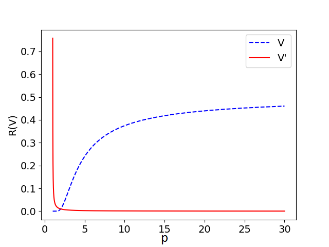
Next we consider monotonicity and majoritarity.

Here we apply our general model to a continuous model of budgeting. Several budgeting methods exist in the literature [32, 8, 14]; we also mention related work on probabilistic social choice [15]. Here we concentrate on a model, termed continuous participatory budgeting, in which fractional funds shall be allocated to several divisible items (in contrast to the non-divisible model of participatory budgeting [18], in which items come with cost, and an item cannot be partially funded):⁶⁶ 6 This model is sometimes also referred to as Pie Chart voting [48]. Specifically, individual financial statement items are grouped by cost centers or departments, and there is a given, fixed budget limit. In contrast to related models [36, 28], we do not assume a fixed set of alternatives provided to the agents to choose from. Rather, every agent may propose a set of alternatives, (represented, e.g., by a string) and an allocation of funds between them.

Utilizing Plott’s theorem [50], that provides a full characterization of Condorcet winners in euclidean spaces, we conclude the following:

In fact, as follows from the literature on spatial models [27], a Condorcet winner exists with probability zero, and the Condorcet cycle usually spans over almost the entire domain.

In contrast, with regards to $L_{p}$ aggregators, since $f(x)=\sum_{i\in[n]}\left\|x-v_{i}\right\|^{p}$ is continuous over the compact domain $\Delta_{m-1}$, it follows that there always exists an element in $X=(\Delta_{m-1},\left\|\cdot\right\|_{p})$ that minimizes $f$. Furthermore, when the ideal points $v_{1},...,v_{n}$ are not collinear (i.e., they do not lie on the same line), it holds that $f$ is positive and strictly convex in $\Delta_{m-1}$, hence obtains a unique minimum (we refer the reader to [63] for elaborate discussion for the case of $p=1$).

The situation here generalizes the situation of $1$-dimensional Euclidean elections described in Section 4, as a $1$-simplex is a $1$-dimensional Euclidean space. From similar reasons as discussed in Section 4 (specifically, the convexity and compactness of $\Delta_{m-1}$), efficient computation for $L_{p}$ aggregation follows by using gradient descent.

Majoritarity holds for Condorcet aggregation and for $L_{1}$ aggregation.

We consider social welfare functions, where the input for an aggregation method is a set of $n$ linear orders and the output of an aggregation method is another linear order. A relevant metric space in this setting is the set of all permutations $X=S_{z}$ over a set of $z$ underlying alternatives, equipped with the metric $d$ induced by swaps of consecutive alternatives (other options are natural for future study).

As for $L_{\infty}$, it is equivalent to the NP-hard Adjacent Element Swap Centre Permutation problem [51, Corollary 1]. Thus $L_{\infty}$ is NP-hard here as well. This fact also follows from Biedl et al. [11].

The following result shows that, for this setting, $L_{p}$ is NP-hard for any $p\geq 1$.

We conjecture that also Condorcet aggregation is NP-hard for this setting, however proving it seems to be quite tricky.

The next example demonstrates that $L_{p}$ aggregation is not monotone for any $p>1$.

Next we consider majoritarity.

Here we consider selecting a committee from a given set of candidates.

First, recall the definition of the median element [43]: Consider an election $E$ based on $n$ ideal elements $V=\{v_{1},\ldots,v_{n}\}$, $v_{i}\in X$. Then, the median element is the element $x\in X$ which contains exactly those alternatives $a\in A$ for which $|\{v\in V:a\in v\}|\geq n/2$. That is, the median element is the unique element containing exactly those alternatives with weak voter majority support.

For $X=2^{A}$, finding $L_{\infty}(V)$ is equivalent to the NP-hard Closest String problem [35]. We also mention that it is equivalent to the variable number of winners counterpart of minimax approval voting [13].

Chen et al. [20], using a slightly different jargon, prove that $L_{p}$ aggregation in NP-hard for all values of $p>1$.

While $L_{p}$ aggregation always exist for this setting, the next example demonstrates that Condorcet winners do not always exist for this application.

Condorcet aggregation for this application can be phrased also as a Condorcet-consistent aggregation method for a binary combinatorial domain with top-based input, where the completion principle is based on the Hamming distance (see, e.g., [21]). Condorcet aggregation was studied by Darmann [22] which demonstrated the computational intractability of a related problem [22, Theorem 3.7].

We note that for committee election, only one committee may be a Condorcet winner: namely the one obtained by the majority voting rule, i.e. taking each alternative selected in a majority of preferences. Indeed, for any other committee, there is no strict majority against adding or removing an “unpopular” alternative. However, this is a necessary condition only, and it remains to decide if such committee actually is a Condorcet winner.

Next we consider majoritarity.

References

- [1] Ali, A., Meilă, M.: Experiments with Kemeny ranking: What works when? Mathematical Social Sciences 64(1), 28–40 (2012)
- [2] Alsina, V., Martí, J.L.: The birth of the CrowdLaw movement: Tech-based citizen participation, legitimacy and the quality of lawmaking. Analyse & Kritik 40(2), 337–358 (2018)
- [3] Anshelevich, E., Bhardwaj, O., Elkind, E., Postl, J., Skowron, P.: Approximating optimal social choice under metric preferences. AI 264, 27–51 (2018)
- [4] Anshelevich, E., Postl, J.: Randomized social choice functions under metric preferences. Journal of Artificial Intelligence Research 58, 797–827 (2017)
- [5] Arrow, K.J.: Social choice and individual values. Yale university press (1951)
- [6] Assembly, N.C.: Declaration of the rights of man and of the citizen (1789)
- [7] Aziz, H., Faliszewski, P., Grofman, B., Slinko, A., Talmon, N.: Egalitarian committee scoring rules. In: Proceedings of IJCAI ’18. pp. 56–62 (2018)
- [8] Aziz, H., Lee, B., Talmon, N.: Proportionally representative participatory budgeting: Axioms and algorithms. In: Proceedings of AAMAS ’18 (2018)
- [9] Barbera, S., Bossert, W., Pattanaik, P.K.: Ranking sets of objects (2004)
- [10] Behrens, J., Kistner, A., Nitsche, A., Swierczek, B.: The principles of liquidfeedback (2014)
- [11] Biedl, T., Brandenburg, F.J., Deng, X.: On the complexity of crossings in permutations. Discrete Mathematics 309(7), 1813–1823 (2009)
- [12] Black, D.: On the rationale of group decision-making. Journal of political economy 56(1), 23–34 (1948)
- [13] Brams, S., Fishburn, P.C.: Approval voting. Springer (2007)
- [14] Brandl, F., Brandt, F., Peters, D., Stricker, C., Suksompong, W.: Donor coordination: Collective distribution of individual contributions (2019), unpublished manuscript.
- [15] Brandt, F.: Rolling the dice: Recent results in probabilistic social choice. In: Endriss, U. (ed.) Trends in Computational Social Choice. AI Access (2017)
- [16] Brill, M., Talmon, N.: Pairwise liquid democracy. In: Proceedings of IJCAI ’18. pp. 137–143 (2018)
- [17] Bullen, P.S.: Handbook of means and their inequalities (2013)
- [18] Cabannes, Y.: Participatory budgeting: a significant contribution to participatory democracy. Environment and urbanization 16(1), 27–46 (2004)
- [19] Caragiannis, I., Nath, S., Procaccia, A.D., Shah, N.: Subset selection via implicit utilitarian voting. Journal of Artificial Intelligence Research 58, 123–152 (2017)
- [20] Chen, J., Hermelin, D., Sorge, M.: On computing centroids according to the -norms of hamming distance vectors. arXiv preprint arXiv:1807.06469 (2018)
- [21] Chevaleyre, Y., Endriss, U., Lang, J., Maudet, N.: Preference handling in combinatorial domains: From AI to social choice. AI magazine 29(4), 37 (2008)
- [22] Darmann, A.: How hard is it to tell which is a Condorcet committee? Mathematical social sciences 66(3), 282–292 (2013)
- [23] Duddy, C., Piggins, A., Zwicker, W.: Aggregation of binary evaluations: a Borda-like approach. Social Choice and Welfare 46(2), 301–333 (2016)
- [24] Duncan, B.: The theory of committees and elections (1958)
- [25] Elkind, E., Faliszewski, P., Slinko, A.: Distance rationalization of voting rules. Social Choice and Welfare 45(2), 345–377 (2015)
- [26] Endriss, U., Grandi, U.: Graph aggregation. AI 245, 86–114 (2017)
- [27] Enelow, J.M., Hinich, M.J.: The spatial theory of voting: An introduction (1984)
- [28] Fain, B., Goel, A., Munagala, K.: The core of the participatory budgeting problem. In: Proceedings of WINE ’16. pp. 384–399 (2016)
- [29] Fain, B., Goel, A., Munagala, K., Sakshuwong, S.: Sequential deliberation for social choice. In: Proceedings of WINE ’17. pp. 177–190 (2017)
- [30] Faliszewski, P., Skowron, P., Slinko, A., Talmon, N.: Multiwinner rules on paths from k-Borda to Chamberlin-Courant. In: Proceedings of IJCAI ’17. pp. 192–198 (2017)
- [31] Faliszewski, P., Skowron, P., Slinko, A., Talmon, N.: Multiwinner voting: A new challenge for social choice theory. In: Endriss, U. (ed.) Trends in Computational Social Choice. AI Access Foundation (2017)
- [32] Faliszewski, P., Talmon, N.: A framework for approval-based budgeting methods. arXiv preprint arXiv:1809.04382 (2018)
- [33] Faliszewski, P., Slinko, A., Talmon, N.: The complexity of multiwinner voting rules with variable number of winners. arXiv preprint arXiv:1711.06641 (2017)
- [34] Feldman, M., Fiat, A., Golomb, I.: On voting and facility location. In: Proceedings of the 2016 ACM Conference on Economics and Computation. pp. 269–286 (2016)
- [35] Frances, M., Litman, A.: On covering problems of codes. Theory of Computing Systems 30(2), 113–119 (1997)
- [36] Garg, N., Kamble, V., Goel, A., Marn, D., Munagala, K.: Collaborative optimization for collective decision-making in continuous spaces. In: Proceedings of WWW ’17. pp. 617–626 (2017)
- [37] Gershkov, A., Moldovanu, B., Shi, X.: Monotonic norms and orthogonal issues in multidimensional voting (2018)
- [38] Gershkov, A., Moldovanu, B., Shi, X.: Voting on multiple issues: What to put on the ballot? Theoretical Economics 14(2), 555–596 (2019)
- [39] Goel, A., Krishnaswamy, A.K., Sakshuwong, S., Aitamurto, T.: Knapsack voting. Collective Intelligence (2015)
- [40] Goel, A., Krishnaswamy, A.K., Munagala, K.: Metric distortion of social choice rules: Lower bounds and fairness properties. In: EC ’17. pp. 287–304 (2017)
- [41] Kilgour, M.: Approval elections with a variable number of winners. Theory and Decision 81(2), 1–13 (2016)
- [42] Lang, J., Xia, L.: Voting in combinatorial domains (2016)
- [43] Meir, R.: Strategic voting (synthesis lectures on AI and ML) (2018)
- [44] Meir, R., Procaccia, A.D., Rosenschein, J.S.: Algorithms for strategyproof classification. Artificial Intelligence 186, 123–156 (2012)
- [45] Miller, J.C.: A program for direct and proxy voting in the legislative process. Public choice 7(1), 107–113 (1969)
- [46] Moulin, H., Brandt, F., Conitzer, V., Endriss, U., Procaccia, A.D., Lang, J.: Handbook of Computational Social Choice. Cambridge University Press (2016)
- [47] Pennecchi, F., Callegaro, L.: Between the mean and the median: the Lp estimator. Metrologia 43(3), 213 (2006)
- [48] Peters, D.: Fair Division of the Commons. Ph.D. thesis, University of Oxford (2019)
- [49] Peters, H., van der Stel, H., Storcken, T.: Generalized median solutions, strategy-proofness and strictly convex norms. Zeitschrift für Operations Research 38(1), 19–53 (1993)
- [50] Plott, C.R.: A notion of equilibrium and its possibility under majority rule. The American Economic Review 57(4), 787–806 (1967)
- [51] Popov, V.Y.: Multiple genome rearrangement by swaps and by element duplications. Theoretical Computer Science 385(1-3), 115–126 (2007)
- [52] Procaccia, A.D., Rosenschein, J.S.: The distortion of cardinal preferences in voting. In: Proceedings of CIA ’06. pp. 317–331 (2006)
- [53] Procaccia, A.D., Tennenholtz, M.: Approximate mechanism design without money. In: Proceedings of EC ’09. pp. 177–186 (2009)
- [54] Schiavinotto, T., Stützle, T.: A review of metrics on permutations for search landscape analysis. Computers & operations research 34(10), 3143–3153 (2007)
- [55] Sen, A.: Social choice theory. Handbook of math. economics 3, 1073–1181 (1986)
- [56] Shahaf, G., Shapiro, E., Talmon, N.: Sybil-resilient reality-aware voting. arXiv preprint arXiv:1807.11105 (2018)
- [57] Shahaf, G., Shapiro, E., Talmon, N.: Aggregation over metric spaces: Proposing and voting in elections, budgeting, and legislation. In: Proceedings of ADT ’19 (2019)
- [58] Shapiro, E., Talmon, N.: Incorporating reality into social choice. In: Proceedings of AAMAS ’18. pp. 1188–1192 (2018)
- [59] Shapiro, E.: Point: foundations of e-democracy. Communications of the ACM 61(8), 31–34 (2018)
- [60] Skowron, P., Elkind, E.: Social choice under metric preferences: Scoring rules and stv. In: Proceedings of AAAI ’17. pp. 706–712 (2017)
- [61] Slavkovik, M., Jamroga, W.: Iterative judgment aggregation. In: Proceedings of ECAI ’16. pp. 1528–1536 (2016)
- [62] Sposito, V.: Some properties of Lp-estimation. Robust Regression: Analysis and Applications (1990)
- [63] Vardi, Y., Zhang, C.H.: The multivariate L1-median and associated data depth. Proceedings of the National Academy of Sciences 97(4), 1423–1426 (2000)