Stability Conditions for Cluster Synchronization in Networks of Heterogeneous Kuramoto Oscillators

Tommaso Menara Giacomo Baggio Danielle S. Bassett Fabio Pasqualetti ^†^†thanks: This material is based upon work supported in part by ARO award 71603NSYIP, and in part by NSF awards BCS1430279 and BCS1631112.^†^†thanks: Tommaso Menara, Giacomo Baggio and Fabio Pasqualetti are with the Department of Mechanical Engineering, University of California at Riverside, {tomenara, gbaggio, fabiopas}@engr.ucr.edu. Danielle S. Bassett is with the Department of Bioengineering, the Department of Electrical and Systems Engineering, the Department of Physics and Astronomy, the Department of Psychiatry, and the Department of Neurology, University of Pennsylvania, dsb@seas.upenn.edu.

Abstract

In this paper we study cluster synchronization in networks of oscillators with heterogenous Kuramoto dynamics, where multiple groups of oscillators with identical phases coexist in a connected network. Cluster synchronization is at the basis of several biological and technological processes; yet the underlying mechanisms to enable cluster synchronization of Kuramoto oscillators have remained elusive. In this paper we derive quantitative conditions on the network weights, cluster configuration, and oscillators’ natural frequency that ensure asymptotic stability of the cluster synchronization manifold; that is, the ability to recover the desired cluster synchronization configuration following a perturbation of the oscillators’ states. Qualitatively, our results show that cluster synchronization is stable when the intra-cluster coupling is sufficiently stronger than the inter-cluster coupling, the natural frequencies of the oscillators in distinct clusters are sufficiently different, or, in the case of two clusters, when the intra-cluster dynamics is homogeneous. We illustrate and validate the effectiveness of our theoretical results via numerical studies.

Index Terms:

Biological neural network, limit cycle, network theory, nonlinear dynamical systems, stability.

I Introduction

Synchronization refers broadly to patterns of coordinated activity that arise spontaneously or by design in several natural and man-made systems [1, 2, 3]. Examples include coherent firing of neuronal populations in the brain [4], coordinated flashing of fireflies [5], flocking of birds [6], exchange of signals in wireless networks [7], consensus in multi-agent systems [8], and power generation in the smart grid [9]. Synchronization enables complex functions: while some systems require complete (or full) synchronization among all the components in order to function properly, others rely on cluster (or partial) synchronization, where different groups exhibit different, yet synchronized, internal behaviors [10].

While studies of full synchronization are numerous and have generated a rich literature, e.g., see [11, 12, 13], conditions explaining the onset of cluster synchronization and its properties are less well understood. Such conditions are necessary for the analysis and, more importantly, the control of synchronized activity across biological [14, 15, 16] and technological [17] systems. For instance, a deeper understanding of the mechanisms enabling cluster synchronization might not only shed light on the nature of the healthy human brain [18], but also enable and guide targeted interventions for patients with neurological disorders, such as epilepsy [19] and Parkinson’s disease [20].

We study cluster synchronization in networks of oscillators with Kuramoto dynamics [21], which, despite their apparent simplicity, are particularly suited to represent complex synchronization phenomena in neural systems [22], as well as in many other natural and technological systems [9]. Although our study and modeling choices are guided by the practical need to understand and control patterns of synchronized functional activity in the human brain, as they naturally arise in healthy and diseased populations [23, 24], in this paper we focus on developing the mathematical foundations of a quantitative approach to the analysis and control of cluster synchronization in a weighted network of Kuramoto oscillators. In particular, we derive conditions on the oscillators’ coupling and their natural frequencies that guarantee the stability of an arbitrary cluster configuration.

Related work Cluster synchronization, where multiple synchronized groups of oscillators coexist in a connected network, is an exciting phenomenon that has attracted the attention of the physics, dynamical systems, and controls communities, among others. Existing work on this topic has shown that cluster-synchronized states can be linked to the existence of certain network symmetries [25, 26, 27, 28, 29] or symmetries in the nodes’ dynamics [30]. More recently, in [31, 32], the stability of cluster states corresponding to network symmetries is addressed with the Master Stability Function approach [33]. In contrast to this previous work, [34] combines network symmetries with contraction analysis to study the stability of synchronized states. Further studies relating contraction properties and cluster synchronization are conducted in [35, 36]. Finally, control algorithms for cluster synchronization are developed in [37, 38]. To the best of our knowledge, however, the above studies are not applicable to oscillators with Kuramoto dynamics, which we study in this work.

A few papers have studied cluster synchronization of Kuramoto oscillators. Specifically, in [39, 40] the authors provide invariance conditions for an approximate definition of cluster synchronization and for particular types of networks. Invariance of exact cluster synchronization, which is the notion used in this paper, is also studied in [41, 42]. Stability of exact cluster synchronization is investigated in [43] where, however, only the restrictive case of two clusters for identical Kuramoto oscillators with inertia is considered, and in [44], where only implicit and numerical stability conditions are provided. To the best of our knowledge, our work presents the first explicit analytical conditions for the (local) stability of the cluster synchronization manifold in sparse and weighted networks of heterogeneous Kuramoto oscillators.

Paper contribution The main contribution of this paper is to characterize conditions for the stability of cluster synchronization in networks of oscillators with Kuramoto dynamics. We consider a notion of exact cluster synchronization, where the phases of the oscillators within each cluster remain equal to each other over time, and different from the phases of the oscillators in the other clusters. We derive three conditions. First, we show that the cluster synchronization manifold is locally exponentially stable when the intra-cluster coupling is sufficiently stronger than the inter-cluster coupling. We quantify this tradeoff using the theory of perturbation for dynamical systems together with the invariance properties of cluster synchronization. Second, through a Lyapunov argument, we show that the cluster synchronization manifold is locally exponentially stable when the natural frequencies of the oscillators in disjoint clusters are sufficiently different (in their limit to infinity). Third, we focus on the case of two clusters, and provide a quantitative condition on the network weights and oscillators’ natural frequency for the stability of the cluster synchronization manifold. This analysis shows that asymptotic stability of the cluster synchronization manifold is guaranteed for weak inter-cluster weights, sufficiently different natural frequencies, or even homogeneous intra-cluster configurations.

As minor contributions, we provide examples showing that network symmetries are not necessary for cluster synchronization of Kuramoto oscillators, and a sufficient condition guaranteeing the absence of stable synchronization submanifolds.

Paper organization The rest of the paper is organized as follows. Section II contains our problem setup and some preliminary notions. Section III contains our main results; that is, our conditions for the stability of the cluster synchronization manifold in Kuramoto networks. Finally, section IV concludes the paper, and the Appendix contains the proofs of our results.

Mathematical notation The set $\mathbb{R}_{>0}$ (resp. $\mathbb{R}_{<0}$ ) denotes the positive (resp. negative) real numbers, whereas the sets $\mathbb{S}^{1}$ and $\mathbb{T}^{n}$ denote the unit circle and the $n$ -dimensional torus, respectively. The vector of all ones is represented by $\mathds{1}$ . We let $O(f)$ denote the order of the function $f$ . Further, we denote a positive (resp. negative) definite matrix $A$ with $A\succ 0$ (resp. $A\prec 0$ ). We indicate the smallest (resp. largest) eigenvalue of a symmetric matrix with $\lambda_{\text{min}}(\cdot)$ (resp. $\lambda_{\text{max}}(\cdot)$ ). A (block-)diagonal matrix is represented by ( $\mathrm{blk}\text{-})\mathrm{diag}(\cdot)$ . We let $\|\cdot\|$ denote the $\ell^{2}$ -norm, and $\mathsf{i}=\sqrt{-1}$ . Finally, $A^{\dagger}$ represents the Moore-Penrose pseudoinverse of the matrix $A$ .

II Problem setup and preliminary notions

In this work we characterize the stability properties of certain synchronized trajectories arising in networks of oscillators with Kuramoto dynamics. To this aim, let $\mathcal{G}=(\mathcal{V},\mathcal{E})$ be the connected and weighted graph representing the network of oscillators, where $\mathcal{V}=\{1,\dots,n\}$ and $\mathcal{E}\subseteq\mathcal{V}\times\mathcal{V}$ represent the oscillators, or nodes, and their interconnection edges, respectively. Let $A=[a_{ij}]$ be the weighted adjacency matrix of $\mathcal{G}$ , where $a_{ij}\in\mathbb{R}_{>0}$ is the weight of the edge $(i,j)\in\mathcal{E}$ , and $a_{ij}=0$ when $(i,j)\not\in\mathcal{E}$ . The dynamics of $i$ -th oscillator is

\displaystyle\dot{\theta}_{i}=\omega_{i}+\sum_{j\neq i}a_{ij}\sin(\theta_{j}-\theta_{i}),

(1)

where $\omega_{i}\in\mathbb{R}_{>0}$ and $\theta_{i}\in\mathbb{S}^{1}$ denote the natural frequency and the phase of the $i$ -th oscillator. Unless specified differently, we assume that the edge weights are symmetric. That is,

(A1)

The network adjacency matrix satisfies $A=A^{\mathsf{T}}$ .

Assumption (A1) is typical in the study of (cluster) synchronization in networks of Kuramoto oscillators, e.g., see [45, 46, 47], as it facilitates the derivation of stability results. While relaxing this assumption is beyond the scope of this work, we will discuss how our stability results can also be applied to study cluster synchronization with asymmetric network weights (see Remark 5). Finally, since the diagonal entries of the adjacency matrix $A$ do not contribute to the dynamics in (1), we assume that $\mathcal{G}$ does not contain self-loops.

A network exhibits cluster synchronization when the oscillators can be partitioned so that the phases of the oscillators in each cluster evolve identically. To be precise, let $\mathcal{P}=\{\mathcal{P}_{1},\dots,\mathcal{P}_{m}\}$ , with $m>1$ , be a partition of $\mathcal{V}$ , where $\bigcup_{i=1}^{m}\mathcal{P}_{i}=\mathcal{V}$ and $\mathcal{P}_{i}\cap\mathcal{P}_{j}=\emptyset$ if $i\neq j$ . Define the cluster synchronization manifold associated with the partition $\mathcal{P}$ as

\displaystyle\mathcal{S}_{\mathcal{P}}=\{\theta\in\mathbb{T}^{n}\;:\;\theta_{i}=\theta_{j}\text{ for all }i,j\in\mathcal{P}_{k},\,k=1,\dots,m\}.

Then, the network is cluster-synchronized with partition $\mathcal{P}$ when the phases of the oscillators belong to $\mathcal{S}_{\mathcal{P}}$ at all times.

In this paper we characterize conditions on the network weights and the oscillators’ natural frequency that guarantee local exponential stability of the cluster synchronization manifold $\mathcal{S}_{\mathcal{P}}$ , for a given partition $\mathcal{P}$ .¹¹ 1 Loosely speaking, the manifold $\mathcal{S}_{\mathcal{P}}$ is locally exponentially stable if $\theta$ converge to $\mathcal{S}_{\mathcal{P}}$ exponentially fast when $\theta(0)$ is sufficiently close to $\mathcal{S}_{\mathcal{P}}$ . In order to study stability of the cluster synchronization manifold, we assume $\mathcal{S}_{\mathcal{P}}$ to be invariant [48, Chapter 3].²² 2 The manifold $\mathcal{S}_{\mathcal{P}}$ is invariant if $\theta(0)\in\mathcal{S}_{\mathcal{P}}$ implies $\theta\in\mathcal{S}_{\mathcal{P}}$ at all times. In particular, following [42], invariance of $\mathcal{S}_{\mathcal{P}}$ is guaranteed by the following conditions:

(A2)

Given $\mathcal{P}=\{\mathcal{P}_{1},\dots,\mathcal{P}_{m}\}$ , the natural frequencies satisfy $\omega_{i}=\omega_{j}$ for every $i,j\in\mathcal{P}_{k}$ and $k~\in~\{1,\dots,m\}$ ,³³ 3 This condition is necessary for $\mathcal{S}_{\mathcal{P}}$ to be forward invariant, and thus stable [42], and is motivated by observed synchronization phenomena, e.g., see [49]. and
(A3)

The network weights satisfy $\sum_{k\in\mathcal{P}_{\ell}}a_{ik}-a_{jk}=0$ for every $i,j\in\mathcal{P}_{z}$ and $z,\ell\in\{1,\dots,m\}$ , with $z\neq\ell$ .

Thus, in the remainder of the paper we assume that (A2) and (A3) are satisfied for the network partition being considered.

Refer to caption — Fig. 1: Fig. 1 illustrates a network of $6$ oscillators with adjacency matrix as in Fig. 1. In this network, the partition $\mathcal{P}=\{\mathcal{P}_{1},\mathcal{P}_{2}\}$ , which satisfies Assumption (A3), cannot be identified by group symmetries of the network for any choice of the positive weights $\alpha_{1}$ , $\alpha_{2}$ , $\alpha_{3}$ , $\alpha_{4}$ , $\beta_{1}$ and $\beta_{2}$ . The manifold $\mathcal{S}_{\mathcal{P}}$ is invariant whenever the oscillators’ natural frequencies satisfy Assumption (A2). Thus, this example shows that network symmetries are not necessary for cluster synchronization of Kuramoto oscillators.

Remark 1

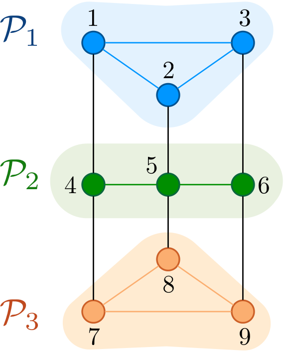
(Network symmetries, equitable partitions, and balanced weights) Conditions to ensure the invariance of the cluster synchronization manifold have been linked to network symmetries, which are defined by the group comprising all node permutations that leave the network topology unchanged, e.g., see [31, 32, 44]. In Fig. 1 we propose a network with two clusters, which are not defined by any group symmetry, that satisfies Assumption (A3) and thus admits an invariant cluster synchronization manifold. This example shows that cluster synchronization of Kuramoto oscillators does not require symmetric networks. Our Assumption (A3), and in fact the equivalent notion of external equitable partition [41], is less restrictive than requiring partitions satisfying group symmetries [50, 51, 52]. Finally, Assumptions (A2) and (A3) are necessary when the natural frequencies in distinct clusters are sufficiently different (see [42] and Remark 2). $\square$

Remark 2

(Invariance of submanifolds of $\mathcal{S}_{\mathcal{P}}$ ) When the network of oscillators is cluster-synchronized (i.e. $\theta(t)\in\mathcal{S}_{\mathcal{P}}$ for all $t\geq 0$ ), submanifolds of $\mathcal{S}_{\mathcal{P}}$ may appear whenever the phases belonging to two (or more) disjoint clusters have equal values (see Fig. 2). Interestingly, the example in Fig. 2 also points out that Assumption (A3) may not be necessary for the invariance of $\mathcal{S}_{\mathcal{P}}$ if the clusters do not evolve with different frequencies (see Assumption (A1) in [42]). In what follows we show that, if the natural frequencies of the oscillators in disjoint clusters are sufficiently different, invariant, and hence stable, submanifolds cannot exist. To see this, assume that the phases of the disjoint clusters $\mathcal{P}_{\ell}$ and $\mathcal{P}_{z}$ remain equal over time. Then, using Assumption (A2) and (A3), the dynamics

	$\displaystyle\dot{\theta}_{\ell}-\dot{\theta}_{z}=\,\omega_{\ell}-\omega_{z}+\sum_{k=1}^{m}$	$\displaystyle\left[\left(\sum_{r\in\mathcal{P}_{k}}a_{\ell r}\right)\sin(\theta_{k}-\theta_{\ell})\right.$
		$\displaystyle\!\!\!-\left.\left(\sum_{r\in\mathcal{P}_{k}}a_{zr}\right)\sin(\theta_{k}-\theta_{z})\right]\!,$		(2)

must be identically zero, where $\theta_{i}$ denotes the phase of any oscillator in $\mathcal{P}_{i}$ . Clearly, if the following inequality holds,

\displaystyle|\omega_{\ell}-\omega_{z}|>2(m-2)\max_{k\neq\ell,z}\left\{\sum_{r\in\mathcal{P}_{k}}a_{\ell r}\,,\sum_{r\in\mathcal{P}_{k}}a_{zr}\!\right\},

(3)

Equation (2) cannot vanish and, consequently, the clusters $\mathcal{P}_{\ell}$ and $\mathcal{P}_{z}$ cannot evolve with the same phases when the network is cluster synchronized.⁴⁴ 4 In (3), we have $(m-2)$ because for $k=z,\ell$ , the sine terms in (2) vanish. More generally, if condition (3) is satisfied for all pairs of clusters, then invariant, and hence stable, cluster synchronization submanifolds cannot exist. $\square$

We conclude with an example showing that the synchronization manifold $\mathcal{S}_{\mathcal{P}}$ is, in general, not globally asymptotically stable due to the existence of multiple invariant sets.

Example 1

(Multiple invariant sets) Consider a Kuramoto network with $2N$ oscillators ( $N\geq 2$ ) and with an adjacency matrix defined as follows⁵⁵ 5 This analysis extends directly to arbitrary weights $a_{ij}=a$ , $a\in\mathbb{R}_{>0}$ . (see Fig. 3 for the case $N=5$ ):

Fig. 3: Fig. 3 shows the network in Example 1 for the case

N=5

. The nodes belonging to partition

\mathcal{P}_{1}

are blue and have natural frequency

\omega_{1}=1

, while the nodes belonging to partition

\mathcal{P}_{2}

are orange and have

\omega_{2}=3

. Fig. 3 illustrates the stability of the set

\mathcal{M}_{\mathcal{P}}

via numerical simulations. We performed

10^{3}

iterations, each one with

\theta(0)

chosen randomly within an angle of

\pm 0.01~[\text{rad}]

from

\mathcal{M}_{\mathcal{P}}

. The thick line represents the mean value among all simulations of the

2

-norm distance between

\theta

and

\mathcal{M}_{\mathcal{P}}

, while the faded area represents the smallest and largest value of the

2

-norm distance between

\theta

and

\mathcal{M}_{\mathcal{P}}

. Fig. 3-3 illustrate the invariance of the set

\mathcal{M}_{\mathcal{P}}

as the phases in the clusters

\mathcal{P}_{1}

and

\mathcal{P}_{2}

evolve respectively with the same frequencies.

\displaystyle a_{ij}=\begin{cases}1,&\text{ if }|i-j|\leq 2,\\ 0,&\text{ otherwise},\end{cases}

with $i,j\in\{1,\dots,2N\}$ (and the convention $2N+\ell\triangleq\ell$ , $-\ell\triangleq 2N+\ell-1$ , for $\ell\in\{1,2\}$ ). Let $\mathcal{P}=\{\mathcal{P}_{1},\mathcal{P}_{2}\}$ , with $\mathcal{P}_{1}=\{1,3,\dots,2N-1\}$ , $\mathcal{P}_{2}=\{2,4,\dots,2N\}$ , and define

\displaystyle\mathcal{M}_{\mathcal{P}}=\{\theta\in\mathbb{T}^{2N}\!\;:\;\!\theta_{i+2}=\theta_{i}+2\pi/N,i=1,\dots,2N-2\}.

It can be verified that Assumption (A3) is satisfied, and that the set $\mathcal{S}_{\mathcal{P}}$ is invariant whenever the natural frequencies satisfy Assumption (A2). Yet, the set $\mathcal{S}_{\mathcal{P}}$ is not the only invariant set. In fact, $\mathcal{M}_{\mathcal{P}}$ is also invariant (we prove this by showing that $\dot{\theta}_{i}=\dot{\theta}_{i+2}$ when $\theta_{i},\theta_{i+2}\in\mathcal{M}_{\mathcal{P}}$ ):

	$\displaystyle\dot{\theta}_{i}$	$\displaystyle=\omega_{i}+\sin(\theta_{i-2}-\theta_{i})+\sin(\theta_{i+2}-\theta_{i})$
		$\displaystyle\;\;\;\;+\sin(\theta_{i-1}-\theta_{i})+\sin(\theta_{i+1}-\theta_{i})$
		$\displaystyle=\omega_{i}+\sin(\theta_{i}-\theta_{i+2})+\sin(\theta_{i+4}-\theta_{i+2})$
		$\displaystyle\;\;\;\;+\sin(\theta_{i+1}-\theta_{i+2})+\sin(\theta_{i+3}-\theta_{i+2})=\dot{\theta}_{i+2},$

where we have used the fact that $\theta_{i+2}-\theta_{i}=2\pi/N$ , and $\omega_{i}=\omega_{j}$ for all $i,j$ in the same cluster. Further, it can be verified numerically that, depending on the number of oscillators $N$ , the set $\mathcal{M}_{\mathcal{P}}$ is also locally stable (see Fig. 3). We conclude that the cluster synchronization manifold $\mathcal{S}_{\mathcal{P}}$ is not, in general, globally asymptotically stable. In what follows we derive conditions guaranteeing local stability of $\mathcal{S}_{\mathcal{P}}$ . $\square$

III Conditions for the stability of the cluster synchronization manifold

In this section we derive sufficient conditions for the local exponential stability of the cluster synchronization manifold. Define the phase difference $x_{ij}=\theta_{j}-\theta_{i}$ , and notice that

\displaystyle\dot{x}_{ij}=\omega_{j}-\omega_{i}+\sum_{z=1}^{n}\left[a_{jz}\sin(x_{jz})-a_{iz}\sin(x_{iz})\right].

(4)

Given a partition $\mathcal{P}=\{\mathcal{P}_{1},\dots,\mathcal{P}_{m}\}$ of the set $\mathcal{V}$ in the graph $\mathcal{G}$ , we define the following graphs (see also Example 2):

(i)

the graph of the $k$ -th cluster, with $k\in\{1,\dots,m\}$ , $\mathcal{G}_{k}=(\mathcal{P}_{k},\mathcal{E}_{k})$ , where $\mathcal{E}_{k}=\{(i,j)\;:\;(i,j)\in\mathcal{E},\;i,j\in\mathcal{P}_{k}\}$ ;
(ii)

a spanning tree $\mathcal{T}_{k}=(\mathcal{P}_{k},\mathcal{E}_{\text{span},k})$ of $\mathcal{G}_{k}$ ;⁶⁶ 6 We assume that $\mathcal{G}$ and its subgraphs $\mathcal{G}_{k}$ are connected. This guarantees the existence of the (connected) spanning trees defined in (ii) and (iii). A graph is connected if there exists a path between any pair of nodes [53].
(iii)

a spanning tree $\mathcal{T}=(\mathcal{V},\mathcal{E}_{\mathcal{T}})$ of $\mathcal{G}$ with $\mathcal{E}_{\mathcal{T}}=\bigcup_{k=1}^{m}\mathcal{E}_{\text{span},k}\cup\mathcal{E}_{\text{inter}}$ , where $\mathcal{E}_{\text{inter}}$ satisfies $|\mathcal{E}_{\text{inter}}|=m-1$ .

Further, we define the following vectors of phase differences:

(iv)

${x}_{\textup{intra}}^{(k)}=[x_{ij}]$ , for all $(i,j)\in\mathcal{E}_{\text{span},k}$ with $i<j$ ,
(v)

${x}_{\textup{intra}}=\left[{x}_{\textup{intra}}^{(1)\mathsf{T}},\dots,{x}_{\textup{intra}}^{(m)\mathsf{T}}\right]^{\mathsf{T}}$ , and
(vi)

${x}_{\textup{inter}}=[x_{ij}]$ , for all $(i,j)\in\mathcal{E}_{\text{inter}}$ with $i<j$ .

It should be noticed that the vectors ${x}_{\textup{intra}}^{(k)}$ , ${x}_{\textup{intra}}$ and ${x}_{\textup{inter}}$ contain, respectively, $n_{\text{intra},k}=|\mathcal{P}_{k}|-1$ , ${n}_{\textup{intra}}=n-m$ and ${n}_{\textup{inter}}=m-1$ entries. Notice that every phase difference can be computed as a linear function of ${x}_{\textup{intra}}$ and ${x}_{\textup{inter}}$ . To see this, let $i,j\in\mathcal{V}$ , and let $\mathrm{p}(i,j)=\{p_{1},\dots,p_{\ell}\}$ be the unique path on $\mathcal{T}$ from $i$ to $j$ . Define $\mathrm{dif}\mathrm{f}(\mathrm{p}(i,j))=\sum_{k=1}^{\ell-1}s_{k}$ , where $s_{k}=x_{p_{k}p_{k+1}}$ if $p_{k}<p_{k+1}$ , and $s_{k}=-x_{p_{k+1}p_{k}}$ otherwise. Then, $x_{ij}=\mathrm{dif}\mathrm{f}(\mathrm{p}(i,j))$ , and the vectors ${x}_{\textup{intra}}$ and ${x}_{\textup{inter}}$ contain a smallest set of phase differences that can be used to quantify synchronization among all of the oscillators in the network.

Let $B=[b_{k\ell}]\in\mathbb{R}^{|\mathcal{V}|\times|\mathcal{E}|}$ denote the oriented incidence matrix of the graph $\mathcal{G}=(\mathcal{V},\mathcal{E})$ , where $\ell$ corresponds to the edge $(i,j)\in\mathcal{E}$ , $b_{k\ell}=1$ if node $k$ is the sink of the edge $\ell$ , $b_{k\ell}=-1$ if $k$ is the source of $\ell$ , and $b_{k\ell}=0$ otherwise.⁷⁷ 7 Node $i$ is the source (resp. sink) of $(i,j)$ if $i<j$ (resp. $i>j$ ). Further, let $B_{k}$ and $B_{\text{span},k}$ denote the incidence matrices of $\mathcal{G}_{k}$ and $\mathcal{T}_{k}$ , respectively. Notice that $B_{\text{span},k}$ is full rank because it is the incidence matrix of an acyclic graph (tree) [53, Theorem 8.3.1]. Let $T_{\text{intra},k}=B_{k}^{\mathsf{T}}(B_{\text{span},k}^{\mathsf{T}})^{\dagger}$ be the unique matrix that maps the phase differences contained in $x_{\text{intra}}^{(k)}$ to all intra-cluster phase differences in the $k$ -th cluster. That is,

\displaystyle x^{(k)}=T_{\text{intra},k}{x}_{\textup{intra}}^{(k)},

(5)

where $x^{(k)}$ contains all phase differences in the cluster $\mathcal{P}_{k}$ .

We conclude this part by rewriting the intra-cluster dynamics in a form that will be useful to prove our results. In particular, from the above discussion and for an intra-cluster phase difference $x_{ij}$ of $x_{\text{intra}}^{(k)}$ , we rewrite (4) as

	$\displaystyle\dot{x}_{ij}=$	$\displaystyle\underbrace{\sum_{z\in\mathcal{P}_{k}}\left[a_{jz}\sin(\mathrm{dif}\mathrm{f}(\mathrm{p}(j,z)))-a_{iz}\sin(\mathrm{dif}\mathrm{f}(\mathrm{p}(i,z)))\right]}_{F_{ij}^{(k)}(x_{\text{intra}}^{(k)})}$
		$\displaystyle+\underbrace{\sum_{z\not\in\mathcal{P}_{k}}\left[a_{jz}\sin(\mathrm{dif}\mathrm{f}(\mathrm{p}(j,z)))-a_{iz}\sin(\mathrm{dif}\mathrm{f}(\mathrm{p}(i,z)))\right]}_{G_{ij}^{(k)}(x_{\text{intra}},x_{\text{inter}})},$		(6)

which leads to

\displaystyle\dot{x}_{\text{intra}}^{(k)}=F^{(k)}(x_{\text{intra}}^{(k)})+G^{(k)}(x_{\text{intra}},x_{\text{inter}}),

(7)

where $F^{(k)}$ is the vector of $F^{(k)}_{ij}$ and $G^{(k)}$ is the vector of $G^{(k)}_{ij}$ , for all $(i,j)\in\mathcal{E}_{\text{span},k}$ with $i<j$ . Finally, by concatenating the dynamics (7) for all clusters, we obtain

\displaystyle\dot{x}_{\text{intra}}=F(x_{\text{intra}})+G(x_{\text{intra}},x_{\text{inter}}).

(8)

Example 2

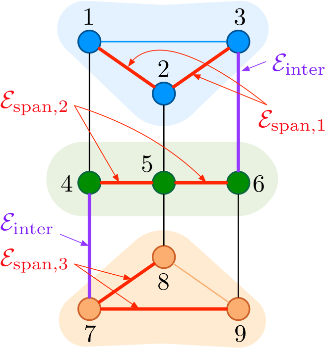
(Illustration of the definitions) We provide here an illustrative example of the definitions introduced in this section. Consider the network in Fig. 4 with partition $\mathcal{P}=\{\mathcal{P}_{1},\mathcal{P}_{2},\mathcal{P}_{3}\}$ , where $\mathcal{P}_{1}=\{1,2,3\}$ , $\mathcal{P}_{2}=\{4,5,6\}$ and $\mathcal{P}_{3}=\{7,8,9\}$ . Fig. 4 illustrates the definitions of spanning trees, together with the edge sets $\mathcal{E}_{\text{span},k}$ $(k=1,2,3)$ , and the inter-cluster edges in $\mathcal{E}_{\text{inter}}=\{(3,6),~(4,7)\}$ . The vectors of intra-cluster differences read as $x_{\text{intra}}^{(1)}=[x_{12}\;x_{23}]^{\mathsf{T}}$ , $x_{\text{intra}}^{(2)}=[x_{45}\>x_{56}]^{\mathsf{T}}$ , and $x_{\text{intra}}^{(3)}=[x_{78}\;x_{79}]^{\mathsf{T}}$ , whereas the vector of inter-cluster differences reads as $x_{\text{inter}}=[x_{36}\;x_{47}]^{\mathsf{T}}$ .

For the partition $\mathcal{P}_{1}$ , order the edges as $\ell_{1}=(1,2)$ , $\ell_{2}=(1,3)$ , and $\ell_{3}=(2,3)$ . Then, a spanning tree is $\mathcal{T}_{1}=(\mathcal{P}_{1},\mathcal{E}_{\text{span},1})$ , with $\mathcal{E}_{\text{span},1}=\{(1,2),(2,3)\}$ , and the (oriented) incidence matrices $B_{1}$ of $\mathcal{G}_{1}$ and $B_{\text{span},1}$ of $\mathcal{T}_{1}$ are

\displaystyle B_{1}=\begin{bmatrix}-1&-1&0\\ 1&0&-1\\ 0&1&1\end{bmatrix},\;\;\;B_{\text{span},1}=\begin{bmatrix}-1&0\\ 1&-1\\ 0&1\end{bmatrix}.

Finally, the matrix $T_{\text{intra},1}=B_{1}^{\mathsf{T}}(B_{\text{span},1}^{\mathsf{T}})^{\dagger}$ satisfies

\displaystyle T_{\text{intra},1}=\begin{bmatrix}1&1&0\\ 0&1&1\end{bmatrix}^{\mathsf{T}}.

$\square$

III-A Local asymptotic stability of $\mathcal{S}_{\mathcal{P}}$ via perturbation theory

In what follows we will make use of perturbation theory of dynamical systems to provide our first stability condition. We first introduce the following instrumental result.

Lemma III.1

(Properties of intra-cluster dynamics) The intra-cluster dynamics (8) satisfies the following properties:

(i)

the Jacobian matrix $J_{\text{intra}}$ of $F(x_{\text{intra}})$ computed at the origin is Hurwitz stable and can be written as

\displaystyle J_{\text{intra}}=\left.\frac{\partial F(x_{\text{intra}})}{\partial{x}_{\textup{intra}}}\right|_{x_{\text{intra}}=0}=\mathrm{blk}\text{-}\mathrm{diag}\left(J_{1},\dots,J_{m}\right),

(9)

where, for $k\in\{1,\dots,m\}$ , $T_{\text{intra},k}$ is as in (5) and

\displaystyle J_{k}=-B_{\text{span},k}^{\mathsf{T}}B_{k}\,\mathrm{diag}(\{a_{ij}\}_{(i,j)\in\mathcal{E}_{k}})T_{\text{intra},k}.

(10)

Thus, the origin is an exponentially stable equilibrium of the system $\dot{x}_{\text{intra}}=F(x_{\text{intra}})$ ;

(ii)

There exist constants $\gamma^{(k\ell)}\in\mathbb{R}_{>0}$ such that

\displaystyle\|G^{(k)}({x_{\text{intra}}},x_{\text{inter}})\|\leq\sum_{\ell=1}^{m}\gamma^{(k\ell)}\|{x_{\text{intra}}^{(\ell)}}\|,

(11)

for all $k,\ell\in\{1,\dots,m\}$ . Specifically,

\displaystyle\gamma^{(k\ell)}=2\max_{r}\;n_{\text{intra},r}\,\tilde{\gamma}^{(k\ell)},

(12)

where, for any $i\in\mathcal{P}_{k}$ ,

\displaystyle\tilde{\gamma}^{(k\ell)}=\begin{cases}\displaystyle\sum_{j\in\mathcal{P}_{\ell}}a_{ij},&\text{ if }\ell\neq k,\\ \displaystyle\sum_{\begin{subarray}{c}\ell=1\\ \ell\neq k\end{subarray}}^{m}\sum_{j\in\mathcal{P}_{\ell}}a_{ij},&\text{ otherwise.}\end{cases}

(13)

As formalized in the next theorem, Lemma III.1, together with results on stability of perturbed systems [54, Chapter 9], implies that the origin of (8), and thus the cluster synchronization manifold $\mathcal{S}_{\mathcal{P}}$ , is exponentially stable for some choices of the network weights. Recall that an $M$ -matrix is a real nonsingular matrix $A=[a_{ij}]$ such that $a_{ij}\leq 0$ for all $i\neq j$ and all leading principal minors are positive [55, Chapter 2.5].

Theorem III.2

(Sufficient condition on network weights for the stability of $\mathcal{S}_{\mathcal{P}}$ ) Let $\mathcal{S}_{\mathcal{P}}$ be the cluster synchronization manifold associated with a partition $\mathcal{P}=\{\mathcal{P}_{1},\dots,\mathcal{P}_{m}\}$ of the network $\mathcal{G}$ of Kuramoto oscillators. Let $\gamma^{(k\ell)}$ be the constants defined in (12). Define the matrix $S\in\mathbb{R}^{m\times m}$ as

\displaystyle S=[s_{k\ell}]=\begin{cases}\lambda_{\text{max}}^{-1}(X_{k})-\gamma^{(kk)}&\text{ if }k=\ell,\\ -\gamma^{(k\ell)}&\text{ if }k\neq\ell,\end{cases}

(14)

where $X_{k}\succ 0$ is such that $J_{k}^{\mathsf{T}}X_{k}+X_{k}J_{k}=-I$ , with $J_{k}$ as in (10). If $S$ is an $M$ -matrix, then the cluster synchronization manifold $\mathcal{S}_{\mathcal{P}}$ is locally exponentially stable.

Remark 3

(Family of bounds) In (14), the matrices $X_{k}$ can be selected as the solutions to the Lyapunov equations $J_{k}^{\mathsf{T}}X_{k}+X_{k}J_{k}=-Q_{k}$ , for arbitrary positive definite matrices $Q_{k}$ . Yet, selecting $Q_{k}=I$ for all $k$ yields a tighter stability bound. This follows because (i) if $S$ is an $M$ -matrix, then $S+\Delta$ remains an $M$ -matrix whenever $\Delta$ is a nonnegative diagonal matrix [55, Theorem 2.5.3], and (ii) the ratio $\lambda_{\text{min}}(Q_{k})/\lambda_{\text{max}}(X_{k})$ is maximal whenever $Q_{k}=I$ [54, Exercise 9.1]. $\square$

Theorem III.2 describes a sufficient condition on the network weights for the stability of the cluster synchronization manifold. Loosely speaking, the cluster synchronization manifold is exponentially stable when the intra-cluster coupling (measured by $\lambda_{\text{max}}^{-1}(X_{k})-\gamma^{(kk)}$ ) is sufficiently stronger than the perturbation induced by the inter-cluster connections (measured by $\gamma^{(k\ell)}$ ). In particular, the term $\lambda_{\text{max}}^{-1}(X_{k})$ is proportional to the intra-cluster weights and it is implicitly related to the network topology. In fact, the matrix $X_{k}$ is the solution of a Lyapunov’s equation containing $J_{k}$ , whose spectrum coincides with the stable eigenvalues of the negative Laplacian matrix of the $k$ -th cluster. We refer the interested reader to the proof of Lemma III.1. Finally, we remark that a result akin to Theorem III.2 has been derived in [56], although for interconnected systems whose coupling functions are required to satisfy certain assumptions that fail to hold in the Kuramoto model.

Fig. 5: Fig. 5 illustrates the network of 6 Kuramoto oscillators in Example 3. We identify the clusters

\mathcal{P}_{1}

and

\mathcal{P}_{2}

in blue and orange, respectively. Fig. 5 contains the adjacency matrix of the network in Fig. 5. The parameters

\alpha_{1},\alpha_{2}

, and

\beta

represent the intra-cluster and inter-cluster weights, respectively. Fig. 5 illustrates the stability of the cluster synchronization manifold

\mathcal{S}_{\mathcal{P}}

for

\alpha_{1}=\alpha_{2}=1

and

\beta=0.1

, as predicted by Theorem III.2. Fig. 5 shows that

\mathcal{S}_{\mathcal{P}}

is unstable when

\alpha_{1}=\beta=1

and

\alpha_{2}=0.001

Example 3

(Tradeoff between intra- and inter-cluster weights) Consider the network in Fig. 5 with partition $\mathcal{P}=\{\mathcal{P}_{1},\mathcal{P}_{2}\}$ , where $\mathcal{P}_{1}=\{1,2,3\}$ and $\mathcal{P}_{2}=\{4,5,6\}$ , natural frequencies $\omega_{1}=1$ and $\omega_{2}=6$ for the oscillators in $\mathcal{P}_{1}$ and $\mathcal{P}_{2}$ , and adjacency matrix as in Fig. 5. The parameters $\alpha_{1},\alpha_{2}\in\mathbb{R}_{>0}$ and $\beta\in\mathbb{R}_{>0}$ denote the strength of the intra- and inter-cluster coupling, respectively. Let $\alpha_{1}=\alpha_{2}$ , and construct the matrix $S$ as in Theorem III.2:

\displaystyle S=\begin{bmatrix}\lambda_{\text{max}}^{-1}(X_{1})-\gamma_{11}&-\gamma_{12}\\ -\gamma_{12}&\lambda_{\text{max}}^{-1}(X_{2})-\gamma_{22}\end{bmatrix},

where $X_{k}\succ 0$ is such that $J_{k}^{\mathsf{T}}X_{k}+X_{k}J_{k}=-I$ , $\lambda_{\text{max}}^{-1}(X_{1})=\lambda_{\text{max}}^{-1}(X_{2})=2\,\alpha_{1}$ and, from (12), $\gamma_{ij}=4\,\beta$ for all $i$ , $j$ . By inspecting all leading principal minors, $S$ is an $M$ -matrix if $\alpha_{1}/\beta>4$ , and the cluster synchronization manifold $\mathcal{S}_{\mathcal{P}}$ is exponentially stable (see Fig. 5). We remark that, when $\alpha_{1}\neq\alpha_{2}$ , the synchronization manifold $\mathcal{S}_{\mathcal{P}}$ can become unstable, as we verify numerically in Fig. 5. $\square$

Fig. 6: This Figure shows that the condition in Theorem III.2 leads to conservative stability bounds. For the network in Example 3, we let

\beta=0.1

and plot, as a function of the ratio

\alpha_{1}/\alpha_{2}

, the stable configurations predicted by Theorem III.2 (green) and those found numerically. For each value of

\alpha_{1}/\alpha_{2}

, we assess numerical stability by making use of the Floquet stability theory [57, Chapter 5] and by resorting to statement (i) in Lemma III.4. This is possible because the partition in Example 3 has only two clusters.

The stability condition in Theorem III.2 depends only on the network weights, and typically leads to conservative bounds (see also Fig. 6). To derive refined stability conditions, we next characterize how the natural frequencies of the oscillators affect stability of the cluster synchronization manifold.

III-B Local asymptotic stability of $\mathcal{S}_{\mathcal{P}}$ when the oscillators’ natural frequencies in disjoint clusters are sufficiently different

Natural frequencies play a fundamental role for full and cluster synchronization of Kuramoto oscillators. However, while heterogeneity of the natural frequencies typically impedes full synchronization [47], we will show that cluster synchronization is in fact facilitated when the oscillators in different clusters have sufficiently different natural frequencies. We start with an asymptotic result that is valid for arbitrary networks and partitions, and then improve our results for the case of partitions containing only two clusters.

Theorem III.3

(Stability of $\mathcal{S}_{\mathcal{P}}$ for large natural frequency differences) Let $\mathcal{S}_{\mathcal{P}}$ be the cluster synchronization manifold associated with a partition $\mathcal{P}=\{\mathcal{P}_{1},\dots,\mathcal{P}_{m}\}$ of the network $\mathcal{G}$ of Kuramoto oscillators. Let $\omega_{i}\in\mathbb{R}_{>0}$ be the natural frequency of the oscillators in the cluster $\mathcal{P}_{i}$ , with $i\in\{1,\dots,m\}$ . In the limit $|\omega_{i}-\omega_{j}|\rightarrow\infty$ , for all $i,j\in\{1,\dots,m\}$ , $i\neq j$ , the cluster synchronization manifold $\mathcal{S}_{\mathcal{P}}$ is locally exponentially stable.

Theorem III.3 shows that heterogeneity of the natural frequencies of the oscillators in different clusters facilitates cluster synchronization, independently of the network weights. We remark that a similar behavior was also identified in [58], although with a different method and definition of synchronization.

We next improve upon Theorem III.3 by analyzing the case where the natural frequencies are finite and the partition $\mathcal{P}$ contains only two clusters. To this aim, let $\mathcal{P}=\{\mathcal{P}_{1},\mathcal{P}_{2}\}$ and assume, without loss of generality, that $\omega_{2}\geq\omega_{1}$ , where $\omega_{i}$ is the natural frequency of the oscillators in $\mathcal{P}_{i}$ . Define

\displaystyle\bar{\omega}

\displaystyle=\omega_{2}-\omega_{1},\text{ and }\bar{a}=\sum_{k\in\mathcal{P}_{2}}a_{ik}+\sum_{k\in\mathcal{P}_{1}}a_{jk},

for any $i\in\mathcal{P}_{1}$ and $j\in\mathcal{P}_{2}$ . The next result characterizes the inter-cluster phase difference when the network evolves on the cluster synchronization manifold.

Lemma III.4

(Nominal inter-cluster difference) Let $\mathcal{S}_{\mathcal{P}}$ be the cluster synchronization manifold associated with a partition $\mathcal{P}=\{\mathcal{P}_{1},\mathcal{P}_{2}\}$ of the network $\mathcal{G}$ of Kuramoto oscillators. Let $\theta(0)\in\mathcal{S}_{\mathcal{P}}$ (equivalently, ${x}_{\textup{intra}}(0)=0$ ). Then, if ${x}_{\textup{intra}}=0$ at all times and $\bar{\omega}>\bar{a}$ ,

	$\displaystyle x_{\text{inter}}(t)$	$\displaystyle=\begin{cases}h(t),&\text{ if }t\neq t_{0}+kT,~k\in\mathbb{Z},\\ \pi,&\text{ if }t=t_{0}+kT,~k\in\mathbb{Z}.\end{cases}$
		$\displaystyle\triangleq{x}_{\textup{nom}}(t),$		(15)

where

h(t)=2\tan^{-1}\!\left(\!\frac{\bar{a}+\sqrt{\bar{\omega}^{2}-\bar{a}^{2}}\,\tan\!\left(\frac{\sqrt{\bar{\omega}^{2}-\bar{a}^{2}}}{2}(t+\tau)\right)}{\bar{\omega}}\!\right),

$t_{0}=-\tau+\pi/\sqrt{\bar{\omega}^{2}-\bar{a}^{2}}$ , $T=2\pi/\sqrt{\bar{\omega}^{2}-\bar{a}^{2}}$ , and $\tau\in\mathbb{R}$ is a constant that depends only on $\theta(0)$ . Moreover,

(i)

$x_{\text{nom}}$ is $T$ -periodic with zero time average, and

(ii)

the following inequality holds:

\displaystyle\left|\int_{0}^{t}\cos(x_{\text{nom}}(\tau))\,\mathop{}\!\mathrm{d}\tau\right|\leq\frac{1}{\bar{a}}\log\left(\frac{\bar{\omega}+\bar{a}}{\bar{\omega}-\bar{a}}\right).

(16)

Remark 4

(Constant versus time-varying inter-cluster difference) The values of $\bar{\omega}$ and $\bar{a}$ determine the behavior of the inter-cluster phase difference. In particular, if $\bar{\omega}<\bar{a}$ , then the inter-cluster difference evolves as in (15).⁸⁸ 8 In fact, $\sqrt{\bar{\omega}^{2}-\bar{a}^{2}}$ becomes a complex number and, by recalling that $\tan(\mathsf{i}\alpha)=\mathsf{i}\tanh(\alpha)$ , where $\alpha\in\mathbb{R}$ , in (15) we have $x_{\text{inter}}(t)=2\tan^{-1}((\bar{a}-\sqrt{\bar{a}^{2}-\bar{\omega}^{2}}\,\tanh(\sqrt{\bar{a}^{2}-\bar{\omega}^{2}}(t+\tau)/2))/\bar{\omega})$ . If $\bar{\omega}=\bar{a}$ , (4) reduces to $\dot{x}_{\text{inter}}=\bar{a}-\bar{a}\sin(x_{\text{inter}})$ , which can be integrated:

	$\displaystyle\bar{a}t$	$\displaystyle=\int_{x_{\text{inter}}(0)}^{x_{\text{inter}}(t)}(1-\sin(s))^{-1}\mathrm{d}s$
	$\displaystyle\bar{a}t$	$\displaystyle=\frac{2\sin(x_{\text{inter}}(t)/2)}{\cos(x_{\text{inter}}(t)/2)-\sin(x_{\text{inter}}(t)/2)}+\tau.$		(17)

By substitution, it can be verified that

\displaystyle x_{\text{inter}}(t)

\displaystyle=2\cos^{-1}\!\left(\!\frac{\bar{a}t-\tau+2}{\sqrt{2(\bar{a}t-\tau+1)^{2}+2}}\!\right)\!,

satisfies equation (17). In both cases ( $\bar{\omega}\leq\bar{a}$ ), $x_{\text{inter}}$ converges to the constant value $2\tan^{-1}((\bar{a}-\sqrt{\bar{a}^{2}-\bar{\omega}^{2}})/\bar{\omega})$ as $t$ increases to infinity. In other words, if $\bar{\omega}\leq\bar{a}$ , then the phases of the oscillators in the two clusters evolve with the same frequency, and the oscillators are phase locked (see Fig. 7 and [47, Remark 1]). Instead, if $\bar{\omega}>\bar{a}$ , the clusters evolve with different frequencies, and the inter-cluster phase difference follows a limit cycle (see Fig. 7 and [54, Chapter 2]). $\square$

Fig. 7: For the network in Example 3 with

\alpha_{1}=\alpha_{2}=\beta=1

\bar{a}=2

and

\bar{\omega}=1

, Fig. 7 shows that the clusters are synchronized (as

\|x_{\text{intra}}^{(1)}\|

and

\|x_{\text{intra}}^{(2)}\|

converge to zero), yet all oscillators remain phase locked (

x_{\text{inter}}

converges to a constant). Instead, Fig. 7 shows that the inter-cluster difference follows a limit cycle when

\alpha_{1}=\alpha_{2}=\beta=1

\bar{a}=2

and

\bar{\omega}=6

In the remainder of this section we assume that $\bar{\omega}>\bar{a}$ , so that the clusters evolve with different frequencies (see Remark 4). Leveraging Lemma III.4, we next present a refined condition for the stability of the cluster synchronization manifold.

Theorem III.5

(Sufficient condition on network weights and natural frequencies for the stability of $\mathcal{S}_{\mathcal{P}}$ ) Let $\mathcal{S}_{\mathcal{P}}$ be the cluster synchronization manifold associated with a partition $\mathcal{P}=\{\mathcal{P}_{1},\mathcal{P}_{2}\}$ of the network $\mathcal{G}$ of Kuramoto oscillators. Let $\omega_{i}\in\mathbb{R}_{>0}$ be the natural frequency of the oscillators in the cluster $\mathcal{P}_{i}$ , with $i\in\{1,2\}$ . Let ${J}_{\textup{intra}}$ be as in Lemma III.1, and $J_{\text{inter}}=\partial G(x_{\text{intra}},x_{\text{inter}})/\partial x_{\text{intra}}$ along the trajectory $x_{\text{intra}}=0$ and $x_{\text{inter}}=x_{\text{nom}}$ . The cluster synchronization manifold $\mathcal{S}_{\mathcal{P}}$ is locally exponentially stable if the following inequality holds:

\displaystyle\left(\frac{\bar{\omega}+\bar{a}}{\bar{\omega}-\bar{a}}\right)^{\frac{2}{\bar{a}}\|J_{\text{inter}}\|}<1+\frac{1}{2\lambda_{\text{max}}(X)\|J_{\text{intra}}\|},

(18)

where $X\succ 0$ is the solution of $J_{\text{intra}}^{\mathsf{T}}X+XJ_{\text{intra}}=-I$ .

Theorem III.5 provides a quantitative condition on the network weights and the natural frequencies of the oscillators to ensure stability of the cluster synchronization manifold. It can be shown that (i) when the inter-cluster weights decrease to zero ( $\bar{a}\rightarrow 0$ ) and $\bar{\omega}$ remains bounded, then $\|{J}_{\textup{inter}}\|/\bar{a}$ remains bounded, the left-hand side of (18) converges to $1$ , and the inequality is automatically satisfied, and (ii) when $\bar{\omega}$ grows ( $\bar{\omega}\rightarrow\infty$ ) and the inter-cluster weights remain bounded, the left-hand side of (18) converges to $1$ and the inequality is automatically satisfied. The role of the intra-cluster connections on the stability of $\mathcal{S}_{\mathcal{P}}$ cannot be evaluated directly from (18) because of the dependency of the right-hand side on $\lambda_{\text{max}}(X)$ . The following result, however, suggests that the synchronization manifold may remain exponentially stable when the intra-cluster weights are homogeneous, independently of the inter-cluster weights and the natural frequencies.

Theorem III.6

(Stability of $\mathcal{S}_{\mathcal{P}}$ with homogeneous clusters) Let $\mathcal{S}_{\mathcal{P}}$ be the cluster synchronization manifold associated with a partition $\mathcal{P}=\{\mathcal{P}_{1},\mathcal{P}_{2}\}$ of the network $\mathcal{G}$ of Kuramoto oscillators. Let $\omega_{i}\in\mathbb{R}_{>0}$ be the natural frequency of the oscillators in the cluster $\mathcal{P}_{i}$ , with $i\in\{1,2\}$ . If ${J}_{\textup{intra}}=\alpha I$ , for some constant $\alpha\in\mathbb{R}_{<0}$ , then the cluster synchronization manifold $\mathcal{S}_{\mathcal{P}}$ is locally exponentially stable.

We provide an example that illustrates the stability conditions derived in Theorem III.5.

Fig. 8: For the network in Example 3, Fig. 8 illustrates the stability of

\mathcal{S}_{\mathcal{P}}

when

\alpha_{1}=\alpha_{2}=\beta=\omega_{1}=1

and

\omega_{2}=47

, as predicted by the condition in Theorem III.5. For the same network and weights, Fig. 8 shows the largest value of inter-cluster weights

\beta^{*}

that satisfies (18) with equality. As predicted by Theorem III.3 and Theorem III.5, stability of the cluster synchronization manifold

\mathcal{S}_{\mathcal{P}}

is preserved when

\bar{\omega}

grows with the inter-cluster weights.

Fig. 9: For the network in Example 3, we let

\alpha_{1}=\beta=1

and

\alpha_{2}=10^{-4}

and plot, as a function of

\bar{\omega}

, the stable configurations predicted by Theorem III.5 (green) and those found numerically. For each value of

\bar{\omega}

, we assess numerical stability (in red) by making use of the Floquet stability theory [57, Chapter 5] and by resorting to statement (i) in Lemma III.4. This is possible because the partition in Example 3 contains two clusters. Although condition (18) is conservative, it captures the effect of large

\bar{\omega}

on the stability of

\mathcal{S}_{\mathcal{P}}

Example 4

(Heterogeneity of natural frequencies improves stability of the cluster synchronization manifold) Consider the network of Kuramoto oscillators in Example 3. Fig. 8 illustrates that the cluster synchronization manifold is asymptotically stable when the condition in Theorem III.5 is satisfied. Fig. 8 illustrates the tradeoff in the latter stability condition between the natural frequency $\bar{\omega}$ and the inter-cluster strength measured by $\beta^{*}$ , which denotes the largest inter-cluster weight $\beta$ (see Example 3) such that (18) is still satisfied. Further, we show in Fig. 9 that, while being conservative, condition (18) captures the fact that stability of the cluster synchronization manifold can be recovered by increasing $\bar{\omega}$ . Namely, choosing the same network weights that yield instability as in Fig. 5, we show that stability of the cluster synchronization manifold is recovered as the difference in natural frequencies grows. $\square$

We conclude this section with a discussion of cluster synchronization in asymmetric networks and identical nodes.

Remark 5

(Extension to networks with asymmetric weights) Symmetry of the network weights is typically exploited to provide conditions for the stability of the full synchronization manifold in networks of Kuramoto oscillators [47]. We rely on the symmetry assumption (A1) to derive statement (i) in Lemma III.1, which supports our main theorems. However, these results remain valid for bidirected graphs,⁹⁹ 9 A bidirected graph is a directed graph where $(i,j)\in\mathcal{E}$ implies $(j,i)\in\mathcal{E}$ . The adjacency matrix of a bidirected graph needs not be symmetric. provided that the Jacobian $J_{\text{intra}}$ can be proven to be Hurwitz. In other words, Assumption (A1) is used to guarantee stability of the isolated clusters, and not of the cluster configuration. $\square$

Remark 6

(Cluster synchronization in networks of identical oscillators) This paper focuses on heterogeneous oscillators and leverages mismatches in the natural frequencies and the network weights to characterize the stability of the cluster synchronization manifold. Yet, cluster synchronization can also arise in networks of homogeneous Kuramoto oscillators, where all units have equal natural frequencies and all edges have equal weight (e.g., see Fig. 10). With the exception of Theorem III.3, which is also applicable in the case of identical edge weights, our stability results cannot predict cluster synchronization in networks of identical oscillators, a question that we leave as the subject of future investigation. $\square$

Fig. 10: Fig. 10 illustrates a network of

10

Kuramoto oscillators with partition

\mathcal{P}=\{\mathcal{P}_{1},\mathcal{P}_{2},\mathcal{P}_{3},\mathcal{P}_{4},\mathcal{P}_{5}\}

, where each cluster is color-coded. All oscillators have identical natural frequency

\omega=3

and all edges have unit weight. As illustrated in Fig. 10, the cluster synchronization manifold associated to

\mathcal{P}

is stable, showing that cluster synchronization is possible even in networks of identical Kuramoto oscillators with identical edge weights.

IV Conclusion and future work

In this work we characterize conditions for the stability of cluster synchronization in networks of oscillators with Kuramoto dynamics, where multiple synchronized groups of oscillators coexist in a connected network. We derive conditions showing that the cluster synchronization manifold is locally exponentially stable when (i) the intra-cluster coupling is sufficiently stronger that the inter-cluster coupling, (ii) the differences of natural frequencies of the oscillators in disjoint clusters are sufficiently large, or, (iii) in the case of two clusters, if the intra-cluster dynamics is homogeneous. To the best of our knowledge, our results are the first to characterize the stability of the cluster synchronization manifold in sparse and weighted networks of heterogeneous Kuramoto oscillators.

Directions of future research include the characterization of tighter stability bounds, the design of methods to control the formation of time-varying synchronized clusters, and the extension of Theorem III.5 to an arbitrary number of clusters.

In this section we provide the proofs of the results presented in Section III, together with some instrumental lemmas.

-A Proofs of the results in Section III-A

Proof of Lemma III.1: Proof of statement (i). Notice that the block-diagonal form of the Jacobian matrix $J_{\text{intra}}$ follows directly from the form of $F(x_{\text{intra}})$ in (8). Therefore, the stability of $J_{\text{intra}}$ is equivalent to the stability of the diagonal blocks $J_{k}$ . Let $\theta^{(k)}$ be the vector of $\theta_{i}$ , $i\in\mathcal{P}_{k}$ and, by Assumption (A2), let $\omega_{k}$ be the natural frequency of any oscillator in $\mathcal{P}_{k}$ . From (1), we write the phase dynamics of the $k$ -th cluster as (see [45])

\displaystyle\dot{\theta}^{(k)}=\omega_{k}\mathds{1}-B_{k}\,\mathrm{diag}(\{a_{ij}\}_{(i,j)\in\mathcal{E}_{k}})\sin(B_{k}^{\mathsf{T}}\theta^{(k)}).

Because the phase differences satisfy $x_{\text{intra}}^{(k)}=B_{\text{span},k}^{\mathsf{T}}\theta^{(k)}$ and $x^{(k)}=B_{k}^{\mathsf{T}}\theta^{(k)}$ , we have

\dot{x}_{\text{intra}}^{(k)}=-B_{\text{span},k}^{\mathsf{T}}B_{k}\,\mathrm{diag}(\{a_{ij}\}_{(i,j)\in\mathcal{E}_{k}})\sin(x^{(k)}),

(19)

where we have used the property $B_{\text{span},k}^{\mathsf{T}}\mathds{1}=0$ . Using (5), the Jacobian matrix of (19) computed at $x_{\text{intra}}^{(k)}=0$ reads as

\displaystyle J_{k}=-B_{\text{span},k}^{\mathsf{T}}B_{k}\,\mathrm{diag}(\{a_{ij}\}_{(i,j)\in\mathcal{E}_{k}})T_{\text{intra},k}.

(20)

Recall that the Laplacian matrix of the graph $\mathcal{G}_{k}$ satisfies

\displaystyle\mathcal{L}_{\mathcal{G}_{k}}=B_{k}\,\mathrm{diag}(\{a_{ij}\}_{(i,j)\in\mathcal{E}_{k}})B_{k}^{\mathsf{T}},

and that, because $\mathcal{G}_{k}$ is connected, the eigenvalues of $-\mathcal{L}_{\mathcal{G}_{k}}$ have negative real part, except one single eigenvalue located at the origin with eigenvector $\mathds{1}$ . Define the matrix $W_{k}=[B_{\text{span},k}\;\mathds{1}]^{\mathsf{T}}$ and notice that, because $B_{\text{span},k}^{\mathsf{T}}\mathds{1}=0$ and $B_{\text{span},k}$ being full column rank [53, Theorem 8.3.1], then $W_{k}$ is invertible and $W_{k}^{-1}=[(B_{\text{span},k}^{\mathsf{T}})^{{\dagger}}\;(\mathds{1}^{\mathsf{T}})^{{\dagger}}]$ . Therefore we have

\displaystyle W_{k}(-\mathcal{L}_{\mathcal{G}_{k}})W_{k}^{-1}=\begin{bmatrix}J_{k}&0\\ 0&0\end{bmatrix},

where we have used that $T_{\text{intra},k}=B_{k}^{\mathsf{T}}(B_{\text{span},k}^{\mathsf{T}})^{\dagger}$ in (20). This shows that $J_{k}$ contains only the stable eigenvalues of $-\mathcal{L}_{\mathcal{G}_{k}}$ .

Proof of statement (ii). Notice that, for any $(j,z)\in\mathcal{E}$ with $j\in\mathcal{P}_{k}$ , $z\in\mathcal{P}_{\ell}$ , and $k\neq\ell$ , the difference $\mathrm{dif}\mathrm{f}(\mathrm{p}(j,z))$ in $G_{ij}^{(k)}(x_{\text{inter}},x_{\text{inter}})$ in equation (6) can be rewritten as

\displaystyle\mathrm{dif}\mathrm{f}(\mathrm{p}(j,z))=\mathrm{dif}\mathrm{f}(\mathrm{p}(j,k^{*}))\!+\!\mathrm{dif}\mathrm{f}(\mathrm{p}(k^{*}\!,\ell^{*}))\!+\mathrm{dif}\mathrm{f}(\mathrm{p}(\ell^{*}\!,z)),

where $k^{*}$ and $\ell^{*}$ are such that $\mathrm{p}(k^{*},\ell^{*})$ is the shortest path on $\mathcal{T}$ connecting the clusters $\mathcal{P}_{k}$ and $\mathcal{P}_{\ell}$ . Then,

		$\displaystyle G_{ij}^{(k)}(x_{\text{inter}},x_{\text{inter}})=$
		$\displaystyle\!\sum_{\begin{subarray}{c}\ell=1\\ \ell\neq k\end{subarray}}^{m}\!\sum_{z\in\mathcal{P}_{\ell}}\!\!\left[a_{jz}\!\sin(\mathrm{dif}\mathrm{f}(\mathrm{p}(j,k^{}))\!+\!\mathrm{dif}\mathrm{f}(\mathrm{p}(k^{}\!,\ell^{}))\!+\!\mathrm{dif}\mathrm{f}(\mathrm{p}(\ell^{}\!,z)))\right.$
		$\displaystyle\left.\;\;\;\;\;-a_{iz}\sin(\mathrm{dif}\mathrm{f}(\mathrm{p}(i,k^{}))+\mathrm{dif}\mathrm{f}(\mathrm{p}(k^{}\!,\ell^{}))\!+\mathrm{dif}\mathrm{f}(\mathrm{p}(\ell^{}\!,z)))\right]\!.$

Notice that $\mathrm{dif}\mathrm{f}(\mathrm{p}(i,k^{*}))$ and $\mathrm{dif}\mathrm{f}(\mathrm{p}(j,k^{*}))$ contain only differences in $x_{\text{intra}}^{(k)}$ , and $\mathrm{dif}\mathrm{f}(\mathrm{p}(\ell^{*},z))$ only differences in $x_{\text{intra}}^{(\ell)}$ .

Notice that $\sin(a+b)=\sin(a)+\delta$ , with $|\delta|\leq|b|$ .¹⁰¹⁰ 10 Letting $\delta=\sin(a+b)-\sin(a)$ , we have $|\delta|=|2\sin(\frac{b}{2})\cos(a+\frac{b}{2})|\leq|2\sin(\frac{b}{2})|$ , from which the inequality $|\delta|\leq|b|$ follows. Then,

	$\displaystyle G_{ij}^{(k)}(x_{\text{intra}},x_{\text{inter}})=$	$\displaystyle\sum_{\begin{subarray}{c}\ell=1\\ \ell\neq k\end{subarray}}^{m}\sum_{z\in\mathcal{P}_{\ell}}[a_{jz}\left(\sin(\mathrm{dif}\mathrm{f}(\mathrm{p}(k^{},\ell^{}))+\delta_{jz}\right)$
		$\displaystyle-a_{iz}\left(\sin(\mathrm{dif}\mathrm{f}(\mathrm{p}(k^{},\ell^{}))+\delta_{iz}\right)]$
	$\displaystyle=$	$\displaystyle\!\sum_{\begin{subarray}{c}\ell=1\\ \ell\neq k\end{subarray}}^{m}\!\left(\sum_{z\in\mathcal{P}_{\ell}}[(a_{jz}-a_{iz})\!\sin(\mathrm{dif}\mathrm{f}(\mathrm{p}(k^{},\ell^{})))]\right.$
		$\displaystyle\left.+\sum_{z\in\mathcal{P}_{\ell}}[a_{jz}\delta_{jz}-a_{iz}\delta_{iz}]\right)$
	$\displaystyle\overset{\text{(A3)}}{=}$	$\displaystyle\sum_{\begin{subarray}{c}\ell=1\\ \ell\neq k\end{subarray}}^{m}\sum_{z\in\mathcal{P}_{\ell}}[a_{jz}\delta_{jz}\!-\!a_{iz}\delta_{iz}],$

where $\delta_{jz}$ and $\delta_{iz}$ are upper bounded by $\sqrt{n_{\text{intra},k}}\|x_{\text{intra}}^{(k)}\|+\sqrt{n_{\text{intra},\ell}}\|x_{\text{intra}}^{(\ell)}\|$ . Therefore, we have the following bound:

	$\displaystyle\|G_{ij}^{(k)}\|$	$\displaystyle\leq\,\sum_{\begin{subarray}{c}\ell=1\\ \ell\neq k\end{subarray}}^{m}\left(\sum_{z\in\mathcal{P}_{\ell}}a_{jz}\|\delta_{jz}\|+\sum_{z\in\mathcal{P}_{\ell}}a_{iz}\|\delta_{iz}\|\right)$
		$\displaystyle\overset{\text{(A3)}}{\leq}2\sum_{\begin{subarray}{c}\ell=1\\ \ell\neq k\end{subarray}}^{m}\sum_{z\in\mathcal{P}_{\ell}}a_{jz}\!\left(\sqrt{n_{\text{intra},k}}\\|x_{\text{intra}}^{(k)}\\|+\sqrt{n_{\text{intra},\ell}}\\|x_{\text{intra}}^{(\ell)}\\|\right)$
		$\displaystyle=2\sum_{\ell=1}^{m}\sqrt{n_{\text{intra},\ell}}\,\,\tilde{\gamma}^{(k\ell)}_{ij}\\|{x_{\text{intra}}^{(\ell)}}\\|,$

where

\displaystyle\tilde{\gamma}^{(k\ell)}_{ij}=\begin{cases}\displaystyle\sum_{\begin{subarray}{c}\ell=1\\ \ell\neq k\end{subarray}}^{m}\sum_{z\in\mathcal{P}_{\ell}}a_{jz},&\text{ if }\ell=k,\\ \displaystyle\sum_{z\in\mathcal{P}_{\ell}}a_{jz},&\text{ otherwise.}\end{cases}

To conclude, $\|G^{(k)}\|\leq\sqrt{n_{\text{intra},k}}\max_{(i,j)\in\mathcal{E}_{\text{span},k}}|G_{ij}^{(k)}|$ , and, due to (A3), $\tilde{\gamma}^{(k\ell)}_{ij}=\tilde{\gamma}^{(k\ell)}$ is independent of $i$ and $j$ . Thus,

\displaystyle\|G^{(k)}\|\leq\sum_{\ell=1}^{m}2\max_{r}\,n_{\text{intra},r}\,\tilde{\gamma}^{(k\ell)}\,\|{x_{\text{intra}}^{(\ell)}}\|.

This concludes the proof. $\blacksquare$

Proof of Theorem III.2: The system (8) can be viewed as the perturbation via $G({x}_{\textup{intra}},{x}_{\textup{inter}})$ of ${\dot{x}}_{\textup{intra}}=F({x}_{\textup{intra}})$ , which describes the dynamics of $m$ disjoint networks of oscillators:

\dot{x}_{\text{intra}}^{(k)}=F^{(k)}({x_{\text{intra}}^{(k)}}).

(21)

The origin of each system (21) is an exponentially stable equilibrium, which can be shown with the Lyapunov candidate

V_{k}(x_{\text{intra}})={x_{\text{intra}}^{(k)\mathsf{T}}}P_{k}{x_{\text{intra}}^{(k)}},

where $P_{k}\succ 0$ is such that $J_{k}^{\mathsf{T}}P_{k}+P_{k}J_{k}=-Q_{k}$ for $Q_{k}\succ 0$ . In fact, the derivative of $V$ along the trajectories (21) is

	$\displaystyle\dot{V}_{k}({x_{\text{intra}}^{(k)}})$	$\displaystyle=F^{(k)\mathsf{T}}({x_{\text{intra}}^{(k)}})P_{k}{x_{\text{intra}}^{(k)}}+x_{\text{intra}}^{(k)\mathsf{T}}P_{k}F^{(k)}({x_{\text{intra}}^{(k)}})$
		$\displaystyle=x_{\text{intra}}^{(k)\mathsf{T}}(J_{k}^{\mathsf{T}}P_{k}+P_{k}J_{k})x_{\text{intra}}^{(k)}+O(\\|{x_{\text{intra}}^{(k)}}\\|^{3}),$		(22)

and the latter is strictly negative when $\|{x}_{\textup{intra}}^{(k)}\|\leq r$ and $r\in\mathbb{R}_{>0}$ is sufficiently small. Further, it holds that: (i) $\|\partial V_{k}/\partial x_{\text{intra}}^{(k)}\|\leq 2\lambda_{\text{max}}(P_{k})\|x_{\text{intra}}^{(k)}\|$ , (ii) $\dot{V}_{k}({x_{\text{intra}}^{(k)}})\leq-\lambda_{\text{min}}(Q_{k})\|x_{\text{intra}}^{(k)}\|^{2}$ , and (iii) the perturbation terms $G^{(k)}({x_{\text{intra}}},x_{\text{inter}})$ are linearly bounded in $\|{x_{\text{intra}}^{(k)}}\|$ following statement (ii) in Lemma III.1.

Consider now the following Lyapunov candidate for (8):

V(x_{\text{intra}})=\sum_{k=1}^{m}d_{k}V_{k}({x_{\text{intra}}^{(k)}}),\;\;\;d_{k}>0.

From [54, Chapter 9.5] we have:

\dot{V}(x_{\text{intra}})\leq-\frac{1}{2}(DS+S^{\mathsf{T}}D)\|x_{\text{intra}}\|^{2},

(23)

where $D=\mathrm{diag}(d_{1},\dots,d_{m})$ , and $S$ satisfies

\displaystyle S=[s_{k\ell}]=\begin{cases}\frac{\lambda_{\text{min}}(Q_{k})}{\lambda_{\text{max}}(P_{k})}-\gamma^{(kk)}&\text{ if }k=\ell,\\ -\gamma^{(k\ell)}&\text{ if }k\neq\ell.\end{cases}

(24)

The origin of (8) is locally exponentially stable if $S$ is an $M$ -matrix [54, Lemma 9.7 and Theorem 9.2]. Finally, choosing $Q_{k}=I$ in (24) yields condition (14) in Theorem III.2. $\blacksquare$

-B Proofs of the results in Section III-B

Let $\mathcal{C}$ be the set of connected clusters pairs, that is,

\displaystyle\mathcal{C}=\{(\ell,z)\;:\;\exists\;(i,j)\in\mathcal{E}\text{ with }i\in\mathcal{P}_{\ell},j\in\mathcal{P}_{z},\text{ and }\ell<z\}.

With a slight abuse of notation, for any $(\ell,z)\in\mathcal{C}$ , we define $x^{(\ell z)}=x_{ij}$ , for any node $i\in\mathcal{P}_{\ell}$ and $j\in\mathcal{P}_{z}$ .

Lemma .1

(Linearized intra-cluster dynamics) The linearization of the intra-cluster dynamics (8) around the trajectory $x_{\text{intra}}=0$ and $x_{\text{inter}}=x_{\text{nom}}$ reads as follows:

\displaystyle\dot{x}_{\text{intra}}=\left(J_{\text{intra}}+{J}_{\textup{inter}}\right)x_{\text{intra}},

(25)

where $J_{\text{intra}}$ is defined in Lemma III.1, and

\displaystyle{J}_{\textup{inter}}=\left.\frac{\partial G}{\partial x_{\text{intra}}}\right|_{\shortstack[l]{ $\scriptstyle x_{\text{intra}}=0$ \\ $\scriptstyle x_{\text{inter}}=x_{\text{nom}}$}}\triangleq\sum_{(\ell,z)\in\mathcal{C}}\cos(x^{\,(\ell z)})\,J_{\text{inter}}^{(\ell z)}.

Proof:

Linearization of (8) around the trajectory $(x_{\text{intra}},x_{\text{inter}})=(0,x_{\text{nom}})$ yields $\partial F/\partial x_{\text{intra}}=J_{\text{intra}}$ and $\partial G/\partial x_{\text{intra}}=J_{\text{inter}}$ . The remaining derivatives vanish. That is, $\partial F/\partial x_{\text{inter}}=0$ because $F$ does not depend on $x_{\text{inter}}$ , and $\partial G/\partial x_{\text{inter}}=0$ because of Assumption (A3). In fact, for any intra-cluster difference $x_{ij}$ with $i,j\in\mathcal{P}_{\ell}$ , $\ell\in\{1,\dots,m\}$ ,

\left.\frac{\partial G_{ij}}{\partial x_{\text{inter}}}\right|_{\shortstack[l]{ $\scriptstyle x_{\text{intra}}=0$ \\ $\scriptstyle x_{\text{inter}}=x_{\text{nom}}$}}=\sum_{(\ell,z)\in\mathcal{C}}\cos(x^{\,(\ell z)})\underbrace{\sum_{k\in\mathcal{P}_{z}}[a_{jk}-a_{ik}]}_{=0}=0.

This concludes the proof. ∎

We next characterize an asymptotic property of the inter-cluster differences through the following instrumental result.

Lemma .2

(Asymptotic behavior of the inter-cluster dynamics for large frequency differences) Let $i\in\mathcal{P}_{\ell}$ , $j\in\mathcal{P}_{z}$ , and $\ell\neq z$ . Then, the inter-cluster difference $x_{ij}$ satisfies

\displaystyle\lim_{|\omega_{j}-\omega_{i}|\rightarrow\infty}\;\frac{x_{ij}(t)}{\omega_{j}-\omega_{i}}=t.

(26)

Proof:

Let $\bar{\omega}_{ij}=\omega_{j}-\omega_{i}$ . We rewrite (4) as

	$\displaystyle\dot{x}_{ij}=$	$\displaystyle\,\bar{\omega}_{ij}-(a_{ij}+a_{ji})\sin(x_{ij})$
		$\displaystyle+\sum_{\begin{subarray}{c}k\neq i,j\end{subarray}}\left[a_{jk}\sin(x_{jk})-a_{ik}\sin(x_{ik})\right].$		(27)

From (27), let $\beta=\sum_{\begin{subarray}{c}k\neq i,j\end{subarray}}[a_{jk}+a_{ik}]$ , and

	$\displaystyle\dot{\underline{x}}_{\,ij}$	$\displaystyle=\bar{\omega}_{ij}-(a_{ij}+a_{ji})\sin(\underline{x}_{\,ij})-\beta,$		(28)
	$\displaystyle\dot{\overline{x}}_{ij}$	$\displaystyle=\bar{\omega}_{ij}-(a_{ij}+a_{ji})\sin(\overline{x}_{ij})+\beta,$		(29)

with ${\underline{x}}_{\,ij}(0)={\overline{x}}_{ij}(0)={x}_{ij}(0)$ . Integrating (28) yields

\int_{{x}_{ij}(0)}^{{\underline{x}}_{\,ij}(t)}\frac{\mathop{}\!\mathrm{d}y}{\bar{\omega}_{ij}-(a_{ij}+a_{ji})\sin(y)-\beta}=\int_{0}^{t}\mathop{}\!\mathrm{d}\tau.

(30)

As $|\bar{\omega}_{ij}|$ grows, it holds that $|(a_{ij}+a_{ji})+\beta|<|\bar{\omega}_{ij}|$ . Therefore,

	$\displaystyle\frac{1}{\bar{\omega}_{ij}-(a_{ij}+a_{ji})\sin(y)-\beta}=\frac{1}{\bar{\omega}_{ij}}\left[\frac{1}{1-\frac{(a_{ij}+a_{ji})\sin(y)+\beta}{\bar{\omega}_{ij}}}\right]$
	$\displaystyle=\frac{1}{\bar{\omega}_{ij}}\sum_{k=0}^{\infty}\left[\frac{(a_{ij}+a_{ji})\sin(y)+\beta}{\bar{\omega}_{ij}}\right]^{k}.$

In view of the latter equality, (30) becomes

	$\displaystyle t=$	$\displaystyle\,\frac{{\underline{x}}_{\,ij}(t)-{x}_{ij}(0)}{\bar{\omega}_{ij}}$
		$\displaystyle+\frac{1}{\bar{\omega}_{ij}}\underbrace{\int_{{x}_{ij}(0)}^{{\underline{x}}_{\,ij}(t)}\sum_{k=1}^{\infty}\left[\frac{(a_{ij}+a_{ji})\sin(y)+\beta}{\bar{\omega}_{ij}}\right]^{k}\!\mathop{}\!\mathrm{d}y}_{O\left(\bar{\omega}_{ij}^{-1}\right)},$

or, equivalently,

\displaystyle{\underline{x}}_{\,ij}(t)=\,\bar{\omega}_{ij}\,t+{x}_{ij}(0)+O\left(\bar{\omega}_{ij}^{-1}\right).

(31)

Similarly, the solution of (29) has the form in (31). Finally, using the Comparison Principle [54, Lemma 3.4], it holds that $\underline{x}_{\,ij}(t)\leq x_{ij}(t)\leq\overline{x}_{ij}(t)$ for all $t\geq 0$ . Hence, $\frac{x_{ij}(t)}{\bar{\omega}_{ij}}\to t$ as $|\bar{\omega}_{ij}|\to\infty$ and this concludes the proof. ∎

We are now ready to prove Theorem III.3.

Proof of Theorem III.3: Consider the Lyapunov candidate $V({x}_{\textup{intra}},t)={x}_{\textup{intra}}^{\mathsf{T}}\Gamma(t){x}_{\textup{intra}}$ , and notice that, using (25),

		$\displaystyle\dot{V}({x}_{\textup{intra}},t)=\;\dot{x}_{\text{intra}}^{\mathsf{T}}\Gamma x_{\text{intra}}+x_{\text{intra}}^{\mathsf{T}}\Gamma\dot{x}_{\text{intra}}+x_{\text{intra}}^{\mathsf{T}}\dot{\Gamma}x_{\text{intra}}$
		$\displaystyle\hskip 14.22636pt=x_{\text{intra}}^{\mathsf{T}}\!\left[\vphantom{\sum_{(\ell,z)\in\mathcal{C}}}\,J_{\text{intra}}^{\mathsf{T}}\Gamma+\Gamma J_{\text{intra}}+\dot{\Gamma}\right.$
		$\displaystyle\hskip 11.38092pt\left.+\!\!\!\sum_{(\ell,z)\in\mathcal{C}}\!\!\cos(x^{\,(\ell z)})\!\left(J_{\text{inter}}^{(\ell z)\mathsf{T}}\Gamma+\Gamma J_{\text{inter}}^{(\ell z)}\right)\!\right]\!x_{\text{intra}}\!+\!O(\\|x_{\text{intra}}\\|^{3}).$		(32)

Let

\displaystyle\dot{\Gamma}=-\sum_{(\ell,z)\in\mathcal{C}}\cos(x^{\,(\ell z)})\!\left(J_{\text{inter}}^{(\ell z)\mathsf{T}}\Gamma+\Gamma J_{\text{inter}}^{(\ell z)}\right).

(33)

When the inter-cluster natural frequencies satisfy $|\omega_{i}-\omega_{j}|\rightarrow\infty$ for all $i,j$ , then $\Gamma(t)\rightarrow\Gamma(0)$ for all times $t$ . In fact, integrating both sides of (33) and substituting $\Gamma(t)=\Gamma(0)$ yields

	$\displaystyle\int_{0}^{t}\!\dot{\Gamma}\mathop{}\!\mathrm{d}\tau\!$	$\displaystyle=\Gamma(t)-\Gamma(0)=\Gamma(0)-\Gamma(0)=0$
		$\displaystyle=\!-\!\!\sum_{(\ell,z)\in\mathcal{C}}\int_{0}^{t}\cos(x^{(\ell z)})\left(J_{\text{inter}}^{(\ell z)\mathsf{T}}\Gamma+\Gamma J_{\text{inter}}^{(\ell z)}\right)\mathop{}\!\mathrm{d}\tau$
		$\displaystyle=\!-\!\!\sum_{(\ell,z)\in\mathcal{C}}\!\!\left(J_{\text{inter}}^{(\ell z)\mathsf{T}}\Gamma(0)+\Gamma(0)J_{\text{inter}}^{(\ell z)}\right)\!\int_{0}^{t}\!\cos(x^{(\ell z)})\mathop{}\!\mathrm{d}\tau,$

which holds true because $\int\cos(x^{(\ell z)})\mathop{}\!\mathrm{d}\tau=0$ due to Lemma .2. Because ${J}_{\textup{intra}}$ is stable, we conclude that, when the inter-cluster natural frequencies satisfy $|\omega_{i}-\omega_{j}|\rightarrow\infty$ for all $i,j$ , $\dot{\Gamma}=0$ , and there exists $\Gamma(0)$ such that (32) is strictly negative. This concludes the proof of the claimed statement. $\blacksquare$

Proof of Lemma III.4: When ${x}_{\textup{intra}}=0$ , the differential equation (27) reduces to $\dot{x}_{\text{inter}}=\bar{\omega}-\bar{a}\sin(x_{\text{inter}})$ , which is a separable differential equation with solution as in (15). To show that the period of (15) is equal to $T=2\pi/\sqrt{\bar{\omega}^{2}-\bar{a}^{2}}$ , we assume, without loss of generality, that $\tau=0$ . It is easy to see that, because $\tan(t)$ is $\pi$ -periodic, $x_{\text{nom}}(t)=x_{\text{nom}}(t+2\pi/\sqrt{\bar{\omega}^{2}-\bar{a}^{2}})$ . Further, notice that the variable substitution $z=x_{\text{nom}}$ in $\int_{0}^{t}\cos(x_{\text{nom}})\,\mathop{}\!\mathrm{d}\tau$ yields

	$\displaystyle\int_{0}^{t}\cos(x_{\text{nom}}(\tau))\,\mathop{}\!\mathrm{d}\tau$	$\displaystyle=\int_{x_{\text{nom}}(0)}^{x_{\text{nom}}(t)}\frac{\cos(z)}{\bar{\omega}-\bar{a}\sin(z)}\,\mathop{}\!\mathrm{d}z$
		$\displaystyle=\frac{1}{\bar{a}}\log\left(\frac{\bar{\omega}-\bar{a}\sin(x(0))}{\bar{\omega}-\bar{a}\sin(x_{\text{nom}}(t))}\right),$		(34)

which implies the bound (16). To prove that $\cos(x_{\text{nom}})$ has zero time average, it suffices to substitute $t=T$ in (34). $\blacksquare$

Proof of Theorem III.5: Consider the Lyapunov candidate $V({x}_{\textup{intra}},t)={x}_{\textup{intra}}^{\mathsf{T}}\Gamma(t){x}_{\textup{intra}}$ , and notice that, using (25),

	$\displaystyle\dot{V}(x_{\text{intra}},t)=$	$\displaystyle\;x_{\text{intra}}^{\mathsf{T}}[\,J_{\text{intra}}^{\mathsf{T}}\Gamma+\Gamma J_{\text{intra}}+\dot{\Gamma}$
	$\displaystyle+$	$\displaystyle\cos(x_{\text{nom}})(J_{\text{inter}}^{\mathsf{T}}\Gamma+\Gamma J_{\text{inter}})\,]x_{\text{intra}}+O(\\|x_{\text{intra}}\\|^{3}).$		(35)

Let $\dot{\Gamma}=-\cos(x_{\text{nom}})(J_{\text{inter}}^{\mathsf{T}}\Gamma+\Gamma J_{\text{inter}})$ and notice that, following [57, Exercise 3.9 and Property 4.2], its solution satisfies

	$\displaystyle\Gamma(t)=$	$\displaystyle\exp\left[{-\int_{0}^{t}\!\cos(x_{\text{nom}}(\tau))\,J_{\text{inter}}^{\mathsf{T}}\,\mathop{}\!\mathrm{d}\tau}\right]\Gamma(0)$
		$\displaystyle\,\cdot\exp\left[{-\int_{0}^{t}\!\cos(x_{\text{nom}}(\tau))J_{\text{inter}}\,\mathop{}\!\mathrm{d}\tau}\right]\!.$

This implies that $V(x_{\text{intra}},t)$ is a Lyapunov function for (25) because, by Lemma III.4, $\int_{0}^{t}\cos(x_{\text{nom}}(\tau))\mathop{}\!\mathrm{d}\tau$ is bounded. Furthermore, notice that

		$\displaystyle\exp\left[{-\int_{0}^{t}\!\cos(x_{\text{nom}}(\tau))\,J_{\text{inter}}^{\mathsf{T}}\,\mathop{}\!\mathrm{d}\tau}\right]$
		$\displaystyle=I+\underbrace{\sum_{k=1}^{\infty}\frac{(J_{\text{inter}}^{\mathsf{T}})^{k}}{k!}\left(-\int_{0}^{t}\!\cos(x_{\text{nom}}(\tau))\,\mathop{}\!\mathrm{d}\tau\right)^{k}}_{\Delta}.$

Thus, (35) can equivalently be written as $\dot{V}=x_{\text{intra}}^{\mathsf{T}}[J_{\text{intra}}^{\mathsf{T}}\Gamma(0)\!+\!\Gamma(0)J_{\text{intra}}\!+\!M\,]x_{\text{intra}}\!+O(\|x_{\text{intra}}\|^{3}),$ where $M=J_{\text{intra}}^{\mathsf{T}}\Delta\Gamma(0)\Delta^{\mathsf{T}}+\Delta\Gamma(0)\Delta^{\mathsf{T}}J_{\text{intra}}+J_{\text{intra}}^{\mathsf{T}}(\Delta\Gamma(0)+\Gamma(0)\Delta)+(\Delta\Gamma(0)+\Gamma(0)\Delta)J_{\text{intra}}.$ using the triangle inequality and Lemma III.4, we obtain

	$\displaystyle\\|\Delta\\|$	$\displaystyle=\left\\|\sum_{k=1}^{\infty}\frac{(J_{\text{inter}}^{\mathsf{T}})^{k}}{k!}\left(-\int_{0}^{t}\!\cos(x_{\text{nom}}(\tau))\,\mathop{}\!\mathrm{d}\tau\right)^{k}\right\\|$
		$\displaystyle\leq\sum_{k=1}^{\infty}\frac{\\|J_{\text{inter}}\\|^{k}}{k!}\left\|\int_{0}^{t}\!\cos(x_{\text{nom}}(\tau))\,\mathop{}\!\mathrm{d}\tau\right\|^{k}$
		$\displaystyle=e^{\left\|\int_{0}^{t}\!\cos(x_{\text{nom}}(\tau))\,\mathop{}\!\mathrm{d}\tau\right\|\\|J_{\text{inter}}\\|}-1\leq e^{\frac{1}{\bar{a}}\log\left(\frac{\bar{\omega}+\bar{a}}{\bar{\omega}-\bar{a}}\right)\\|J_{\text{inter}}\\|}-1.$

Because $J_{\text{intra}}$ is stable, there always exists $\Gamma(0)\succ 0$ such that $J_{\text{intra}}^{\mathsf{T}}\Gamma(0)+\Gamma(0)J_{\text{intra}}=-Q$ for any $Q\succ 0$ . Thus,

\displaystyle\dot{V}\leq

\displaystyle\;(-\lambda_{\text{min}}(Q)+\|M\|)\|x_{\text{intra}}\|^{2}+O(\|x_{\text{intra}}\|^{3}).

(36)

By a simple Lyapunov argument, the cluster synchronization manifold $\mathcal{S}_{\mathcal{P}}$ is locally exponentially stable if $\|M\|<\lambda_{\text{min}}(Q)$ . In addition, $\|M\|$ can be upper bounded as

	$\displaystyle\\|M\\|\leq$	$\displaystyle 2\\|J_{\text{intra}}\\|\\|\Gamma(0)\\|\\|\Delta\\|(\\|\Delta\\|+2)$
	$\displaystyle\leq$	$\displaystyle 2\lambda_{\text{max}}(\Gamma(0))\\|J_{\text{intra}}\\|\left(e^{\frac{2}{\bar{a}}\log\left(\frac{\bar{\omega}+\bar{a}}{\bar{\omega}-\bar{a}}\right)\\|J_{\text{inter}}\\|}-1\right).$

Thus, a sufficient condition for local exponential stability is

\displaystyle 2\lambda_{\text{max}}(\Gamma(0))\|J_{\text{intra}}\|\left(e^{\frac{2}{\bar{a}}\log\left(\frac{\bar{\omega}+\bar{a}}{\bar{\omega}-\bar{a}}\right)\|J_{\text{inter}}\|}-1\right)<\lambda_{\text{min}}(Q),

and because the ratio $\lambda_{\text{min}}(Q)/\lambda_{\text{max}}(\Gamma(0))$ is maximized for $Q=I$ [54, Exercise 9.1], we have

\displaystyle 2\lambda_{\text{max}}(\Gamma(0))\|J_{\text{intra}}\|\left(e^{\frac{2}{\bar{a}}\log\left(\frac{\bar{\omega}+\bar{a}}{\bar{\omega}-\bar{a}}\right)\|J_{\text{inter}}\|}-1\right)<1,

from which condition (18) follows. $\blacksquare$

Proof of Theorem III.6: From (35) and for $\beta\in\mathbb{R}_{>0}$ we have $\dot{V}(x_{\text{intra}},t)=\;x_{\text{intra}}^{\mathsf{T}}[\,J_{\text{intra}}^{\mathsf{T}}\Gamma+\Gamma J_{\text{intra}}\,]x_{\text{intra}}+O(\|x_{\text{intra}}\|^{3})=\;-\beta x_{\text{intra}}^{\mathsf{T}}\Gamma x_{\text{intra}}+O(\|x_{\text{intra}}\|^{3}),$ which is negative in a small neighborhood of the origin. $\blacksquare$

References

[1] M. Girvan and M. E. J. Newman. Community structure in social and biological networks. Proceedings of the National Academy of Sciences, 99(12):7821–7826, 2002.
[2] A. Pikovsky, M. Rosenblum, and J. Kurths. Synchronization: A Universal Concept in Nonlinear Sciences. Cambridge University Press, 2003.
[3] F. L. Lewis, H. Zhang, K. Hengster-Movric, and A. Das. Introduction to synchronization in nature and physics and cooperative control for multi-agent systems on graphs. In Cooperative Control of Multi-Agent Systems, pages 1–21. Springer, 2014.
[4] J. Cabral, E. Hugues, O. Sporns, and G. Deco. Role of local network oscillations in resting-state functional connectivity. Neuroimage, 57(1):130–139, 2011.
[5] A. Moiseff and J. Copeland. A new type of synchronized flashing in a north american firefly. Journal of Insect Behavior, 13(4):597–612, 2000.
[6] I. Giardina. Collective behavior in animal groups: theoretical models and empirical studies. HFSP Journal, 2(4):205–219, 2008.
[7] O. Simeone, U. Spagnolini, Y. Bar-Ness, and S. H. Strogatz. Distributed synchronization in wireless networks. IEEE Signal Processing Magazine, 25(5):81–97, 2008.
[8] F. Garin and L. Schenato. A survey on distributed estimation and control applications using linear consensus algorithms. In Networked Control Systems, LNCIS, pages 75–107. Springer, 2010.
[9] F. Dörfler, M. Chertkov, and F. Bullo. Synchronization in complex oscillator networks and smart grids. Proceedings of the National Academy of Sciences, 110(6):2005–2010, 2013.
[10] F. Sorrentino and E. Ott. Network synchronization of groups. Phys. Rev. E, 76(5):056114, 2007.
[11] S. Boccaletti, V. Latora, Y. Moreno, M. Chavez, and D. U. Hwang. Complex networks: Structure and dynamics. Physics Reports, 424(4-5):175–308, 2006.
[12] N. Chopra and M. W. Spong. On exponential synchronization of Kuramoto oscillators. IEEE Transactions on Automatic Control, 54(2):353–357, 2009.
[13] A. Arenas, A. Díaz-Guilera, J. Kurths, Y. Moreno, and C. Zhou. Synchronization in complex networks. Phys. Rep., 469(3):93–153, 2008.
[14] K. Kaneko. Relevance of dynamic clustering to biological networks. Physica D: Nonlinear Phenomena, 75(1-3):55–73, 1994.
[15] L. Stone, R. Olinky, B. Blasius, A. Huppert, and B. Cazelles. Complex synchronization phenomena in ecological systems. In AIP Conference Proceedings, volume 622, pages 476–488. AIP, 2002.
[16] I. Belykh and M. Hasler. Mesoscale and clusters of synchrony in networks of bursting neurons. Chaos, 21(1):016106, 2011.
[17] J. R. Terry, K. S. Thornburg Jr, D. J. DeShazer, G. D. VanWiggeren, S. Zhu, P. Ashwin, and R. Roy. Synchronization of chaos in an array of three lasers. Phys. Rev. E, 59(4):4036, 1999.
[18] A. Schnitzler and J. Gross. Normal and pathological oscillatory communication in the brain. Nat. Rev. Neurosci., 6(4):285, 2005.
[19] K. Lehnertz, S. Bialonski, M.-T. Horstmann, D. Krug, A. Rothkegel, M. Staniek, and T. Wagner. Synchronization phenomena in human epileptic brain networks. Journal of Neuroscience Methods, 183(1):42–48, 2009.
[20] C. Hammond, H. Bergman, and P. Brown. Pathological synchronization in Parkinson’s disease: networks, models and treatments. Trends in Neurosciences, 30(7):357–364, 2007.
[21] Y. Kuramoto. Self-entrainment of a population of coupled non-linear oscillators. In International symposium on mathematical problems in theoretical physics, pages 420–422, Berlin, Heidelberg, 1975.
[22] A. Daffertshofer and B. van Wijk. On the influence of amplitude on the connectivity between phases. Frontiers in Neuroinformatics, 5:6, 2011.
[23] G. Deco, V. Jirsa, A. R. McIntosh, O. Sporns, and R. Kötter. Key role of coupling, delay, and noise in resting brain fluctuations. Proceedings of the National Academy of Sciences, 106(25):10302–10307, 2009.
[24] F. Váša, M. Shanahan, P. J. Hellyer, G. Scott, J. Cabral, and R. Leech. Effects of lesions on synchrony and metastability in cortical networks. Neuroimage, 118:456–467, 2015.
[25] V. N. Belykh, I. Belykh, and M. Hasler. Hierarchy and stability of partially synchronous oscillations of diffusively coupled dynamical systems. Phys. Rev. E, 62(5):6332, 2000.
[26] A. Y. Pogromsky, G. Santoboni, and H. Nijmeijer. Partial synchronization: from symmetry towards stability. Physica D: Nonlinear Phenomena, 172(1-4):65–87, 2002.
[27] I. Belykh, V. N. Belykh, K. Nevidin, and M. Hasler. Persistent clusters in lattices of coupled nonidentical chaotic systems. Chaos, 13(1):165–178, 2003.
[28] I. Stewart, M. Golubitsky, and M. Pivato. Symmetry groupoids and patterns of synchrony in coupled cell networks. SIAM Journal on Applied Dynamical Systems, 2(4):609–646, 2003.
[29] A. Y. Pogromsky. A partial synchronization theorem. Chaos, 18(3):037107, 2008.
[30] D. Fiore, G. Russo, and M. di Bernardo. Exploiting nodes symmetries to control synchronization and consensus patterns in multiagent systems. Control Systems Letters, 1(2):364–369, 2017.
[31] L. M. Pecora, F. Sorrentino, A. M. Hagerstrom, T. E. Murphy, and R. Roy. Cluster synchronization and isolated desynchronization in complex networks with symmetries. Nature Communications, 5, 2014.
[32] F. Sorrentino, L. M. Pecora, A. M. Hagerstrom, T. E. Murphy, and R. Roy. Complete characterization of the stability of cluster synchronization in complex dynamical networks. Science Advances, 2(4), 2016.
[33] L. M. Pecora and T. L. Carroll. Master stability functions for synchronized coupled systems. Phys. Rev. Lett., 80(10):2109, 1998.
[34] G. Russo and J.-J E. Slotine. Symmetries, stability, and control in nonlinear systems and networks. Phys. Rev. E, 84(4):041929, 2011.
[35] Q. C. Pham and J.-J. Slotine. Stable concurrent synchronization in dynamic system networks. Neural Networks, 20(1):62–77, 2007.
[36] Z. Aminzare, B. Dey, E. N. Davison, and N. E. Leonard. Cluster synchronization of diffusively-coupled nonlinear systems: A contraction based approach. Journal of Nonlinear Science, pages 1–23, 2018.
[37] W. Wu, W. Zhou, and T. Chen. Cluster synchronization of linearly coupled complex networks under pinning control. IEEE Transactions on Circuits and Systems, 56(4):829–839, 2009.
[38] W. Lu, B. Liu, and T. Chen. Cluster synchronization in networks of coupled nonidentical dynamical systems. Chaos, 20(1):013120, 2010.
[39] C. Favaretto, A. Cenedese, and F. Pasqualetti. Cluster synchronization in networks of Kuramoto oscillators. In IFAC World Congress, pages 2433–2438, Toulouse, France, July 2017.
[40] Y. Qin, Y. Kawano, and M. Cao. Partial phase cohesiveness in networks of communitinized Kuramoto oscillators. In European Control Conference, pages 2028–2033, Limassol, Cyprus, 2018.
[41] M. T. Schaub, N. O’Clery, Y. N. Billeh, J.-C. Delvenne, R. Lambiotte, and M. Barahona. Graph partitions and cluster synchronization in networks of oscillators. Chaos, 26(9):094821, 2016.
[42] L. Tiberi, C. Favaretto, M. Innocenti, D. S. Bassett, and F. Pasqualetti. Synchronization patterns in networks of Kuramoto oscillators: A geometric approach for analysis and control. In IEEE Conf. on Decision and Control, pages 481–486, Melbourne, Australia, December 2017.
[43] I. V. Belykh, B. N. Brister, and V. N. Belykh. Bistability of patterns of synchrony in Kuramoto oscillators with inertia. Chaos, 26(9):094822, 2016.
[44] Y. S. Cho, T. Nishikawa, and A. E. Motter. Stable chimeras and independently synchronizable clusters. Phys. Rev. Lett., 119(8):084101, 2017.
[45] A. Jadbabaie, N. Motee, and M. Barahona. On the stability of the Kuramoto model of coupled nonlinear oscillators. In American Control Conference, pages 4296–4301, Boston, MA, USA, June 2004.
[46] F. Dörfler and F. Bullo. Exploring synchronization in complex oscillator networks. In IEEE Conf. on Decision and Control, pages 7157–7170, Maui, Hawaii, USA, 2012. IEEE.
[47] F. Dörfler and F. Bullo. Synchronization in complex networks of phase oscillators: A survey. Automatica, 50(6):1539–1564, 2014.
[48] A. N. Michel, L. Hou, and D. Liu. Stability of Dynamical Systems. Springer, 2008.
[49] D. Mantini, M. G. Perrucci, C. Del Gratta, G. L. Romani, and M. Corbetta. Electrophysiological signatures of resting state networks in the human brain. Proceedings of the National Academy of Sciences, 104(32):13170–13175, 2007.
[50] Z. Ma, Z. Liu, and G. Zhang. A new method to realize cluster synchronization in connected chaotic networks. Chaos, 16(2):023103, 2006.
[51] V. N. Belykh, G. V. Osipov, V. S. Petrov, J. A. K. Suykens, and J. Vandewalle. Cluster synchronization in oscillatory networks. Chaos, 18(3), 2008.
[52] A. B. Siddique, L. Pecora, J. D. Hart, and F. Sorrentino. Symmetry-and input-cluster synchronization in networks. Phys. Rev. E, 97(4):042217, 2018.
[53] C. Godsil and G. F. Royle. Algebraic Graph Theory. Graduate Texts in Mathematics. Springer New York, 2001.
[54] H. K. Khalil. Nonlinear Systems. Prentice Hall, 3 edition, 2002.
[55] R. A. Horn and C. R. Johnson. Topics in Matrix Analysis. Cambridge University Press, 1994.
[56] J. Qin, Q. Ma, H. Gao, Y. Shi, and Y. Kang. On group synchronization for interacting clusters of heterogeneous systems. IEEE Transactions on Cybernetics, 47(12):4122–4133, 2017.
[57] W. J. Rugh. Linear System Theory. Information and System Sciences Series. Prentice Hall, New Jersey, 1993.
[58] C. Favaretto, D. S. Bassett, A. Cenedese, and F. Pasqualetti. Bode meets Kuramoto: Synchronized clusters in oscillatory networks. In American Control Conference, pages 2378–5861, Seattle, WA, May 2017.

	$\displaystyle\|G_{ij}^{(k)}\|$	$\displaystyle\leq\,\sum_{\begin{subarray}{c}\ell=1\\ \ell\neq k\end{subarray}}^{m}\left(\sum_{z\in\mathcal{P}_{\ell}}a_{jz}\|\delta_{jz}\|+\sum_{z\in\mathcal{P}_{\ell}}a_{iz}\|\delta_{iz}\|\right)$
		$\displaystyle\overset{\text{(A3)}}{\leq}2\sum_{\begin{subarray}{c}\ell=1\\ \ell\neq k\end{subarray}}^{m}\sum_{z\in\mathcal{P}_{\ell}}a_{jz}\!\left(\sqrt{n_{\text{intra},k}}\\|x_{\text{intra}}^{(k)}\\|+\sqrt{n_{\text{intra},\ell}}\\|x_{\text{intra}}^{(\ell)}\\|\right)$
		$\displaystyle=2\sum_{\ell=1}^{m}\sqrt{n_{\text{intra},\ell}}\,\,\tilde{\gamma}^{(k\ell)}_{ij}\\|{x_{\text{intra}}^{(\ell)}}\\|,$

	$\displaystyle\\|\Delta\\|$	$\displaystyle=\left\\|\sum_{k=1}^{\infty}\frac{(J_{\text{inter}}^{\mathsf{T}})^{k}}{k!}\left(-\int_{0}^{t}\!\cos(x_{\text{nom}}(\tau))\,\mathop{}\!\mathrm{d}\tau\right)^{k}\right\\|$
		$\displaystyle\leq\sum_{k=1}^{\infty}\frac{\\|J_{\text{inter}}\\|^{k}}{k!}\left\|\int_{0}^{t}\!\cos(x_{\text{nom}}(\tau))\,\mathop{}\!\mathrm{d}\tau\right\|^{k}$
		$\displaystyle=e^{\left\|\int_{0}^{t}\!\cos(x_{\text{nom}}(\tau))\,\mathop{}\!\mathrm{d}\tau\right\|\\|J_{\text{inter}}\\|}-1\leq e^{\frac{1}{\bar{a}}\log\left(\frac{\bar{\omega}+\bar{a}}{\bar{\omega}-\bar{a}}\right)\\|J_{\text{inter}}\\|}-1.$

	$\displaystyle\\|M\\|\leq$	$\displaystyle 2\\|J_{\text{intra}}\\|\\|\Gamma(0)\\|\\|\Delta\\|(\\|\Delta\\|+2)$
	$\displaystyle\leq$	$\displaystyle 2\lambda_{\text{max}}(\Gamma(0))\\|J_{\text{intra}}\\|\left(e^{\frac{2}{\bar{a}}\log\left(\frac{\bar{\omega}+\bar{a}}{\bar{\omega}-\bar{a}}\right)\\|J_{\text{inter}}\\|}-1\right).$

Stability Conditions for Cluster Synchronization in Networks of Heterogeneous Kuramoto Oscillators

Abstract

Index Terms:

I Introduction

II Problem setup and preliminary notions

Remark 1

Remark 2

Example 1

III Conditions for the stability of the cluster synchronization manifold

Example 2

III-A Local asymptotic stability of 𝒮𝒫\mathcal{S}_{\mathcal{P}} via perturbation theory

Lemma III.1

Theorem III.2

Remark 3

Example 3

III-B Local asymptotic stability of 𝒮𝒫\mathcal{S}_{\mathcal{P}} when the oscillators’ natural frequencies in disjoint clusters are sufficiently different

Theorem III.3

Lemma III.4

Remark 4

Theorem III.5

Theorem III.6

Example 4

Remark 5

Remark 6

IV Conclusion and future work

-A Proofs of the results in Section III-A

-B Proofs of the results in Section III-B

Lemma .1

Proof:

Lemma .2

Proof:

References

III-A Local asymptotic stability of $\mathcal{S}_{\mathcal{P}}$ via perturbation theory

III-B Local asymptotic stability of $\mathcal{S}_{\mathcal{P}}$ when the oscillators’ natural frequencies in disjoint clusters are sufficiently different