Dynamical phase diagrams of a love capacity constrained prey-predator model
Evin, Tehran 19839, Iran
2 Center for Network Science, Central European University, H-1051, Budapest, Hungary
3 School of Business, University of Leicester, University Road, Leicester LE1 7RH, United Kingdom
4 GRAPES , rue de la Belle Jardinière 483,
B-4031, Angleur, Belgium
5 Psychological and Brain Science, Indiana University, Bloomington, USA
6 Instituto Argentino de Radioastronomía, CCT La Plata, CONICET, Argentina.
7 Laboratorio de Redes y Sistemas Móviles, FI-UBA, Argentina
8 Scuola di Economia e Statistica, Department of Statistics and Quantitative Methods,
Università degli Studi di Milano-Bicocca, I-20126 Milano, Italy
Abstract
One interesting question in love relationships is: finally, what and when is the end of this love relationship? Using a prey-predator Verhulst-Lotka-Volterra (VLV) model we imply cooperation and competition tendency between people in order to describe a ”love dilemma game”. We select the most simple but immediately most complex case for studying the set of nonlinear differential equations, i.e. that implying three persons, being at the same time prey and predator. We describe four different scenarios in such a love game containing either a one-way love or a love triangle. Our results show that it is hard to love more than one person simultaneously. Moreover, to love several people simultaneously is an unstable state. We find some condition in which persons tend to have a friendly relationship and love someone in spite of their antagonistic interaction. We demonstrate the dynamics by displaying flow diagrams.
1 INTRODUCTION
Empirical studies and theoretical modeling of interacting agents have been the subject of a large body of recent research in statistical physics and applied mathematics [1]. No need to recall (an exhaustive list of references would be impossible neither to print nor read) the flurry of papers on the ”prisoner’s dilemma game” since it was proposed by Flood and Dresher in 1950 [2, 3]. Nowadays, agents are considered to behave on networks rather than on lattices. Their ”opinion evolution” can be imagined to occur according to complex algorithms, but also basing their evolutive behavior on non linear differential equations. Let it be recalled that the Lotka-Volterra differential equation set for preys-predators [4] has been used in various ways to model many types of complex systems, with competitive or cooperation aspects. For instance, outside demography or biology, effects of competition on growth, pertinent in economy and opinion formation [5, 6] taking into account a ”market capacity” [7, 8] has been studied in [9, 10, 11].
As recently pointed out [12], dynamic system theory is useful for describing complex behavior of humans. The usefulness of non linear differential equations is hereby used for outlining possible ”love story” scenarios. The classical Lotka-Volterra equations [4] for prey-predator population evolution is taken as a model for one of the most common human behavior: love. The psychological conditions of a triad of potential lovers is described through an adjacency matrix. The mathematical analysis follows ideas presented elsewhere for economic-financial markets [9, 10, 11], introducing the notion of maximum love capacity, as in Verhulst logistic equation[7, 8], that is, limited resources for a population in a country.
The purpose of the described work here below touches upon a classical aspect of human nature, described by many but rarely touched upon in terms of complex system theories, - yet quite useful in quantitative social sciences, including psychology and cognition [12]. Nevertheless, it is fair to point to a pioneering work on the matter by Strogatz [13]. He considers the evolution of love in a couple. We add that such an evolution depends in an endogenous way of the possible other partners. Moreover, it is reasonable to consider an exogenous constraint: a ”love capacity” concept can also be introduced.
In Sect. 2, we present and develop a generalized Verhulst-Lotka-Volterra model in order to describe the ”love states” of three interacting persons. In Sect. 3, we analyze the four possible interaction schemes, searching for steady states through a fixed point and stability analysis. We present the non trivial dynamical phase diagrams, depending on initial love conditions of the partners. In Sect. 4, we point to the qualitative ”love story” aspects mimicked by our quantifying non-linear dynamics model, - and suggest extensions.
2 METHOD
The classical Lotka-Volterra equations or the predator-prey model equations are used to describe the dynamics of a population made of two species which interact, one as a predator and the other as a prey. The size of populations ( 1 or 2) changes according to the set of equations
| (2.1) |
where ’s and ’s are system parameters.
On the other hand, the simple logistic growth equation also known as the Verhulst equation describes the time evolution of a single species. Interestingly , and realistically, this equation considers the lack of resources in the growth of the population of a species according to the equation
| (2.2) |
where the parameter is related to the available resources for a species.
One can combine these two aspects of a population growth of species to find a generalized model which describes the evolution of the population of several species, on a ”market” with finite resources. The combination of these equations leads to the generalized Verhulst-Lotka-Volterra model [9, 10, 11]
| (2.3) |
In the present case, is the ”size of the love” of the agent i, such that ; is the growth rate for the love when there is no interaction; is the maximum capacity of the love for the agent i. According to psychological aspects, the maximum amount of ”love capacity” is supposed to be such that
similar to market constraints in economy and finance [9, 10, 11]. For simplicity, we may assume that all the lovers have the same growth rate and also assume that the love capacity is .
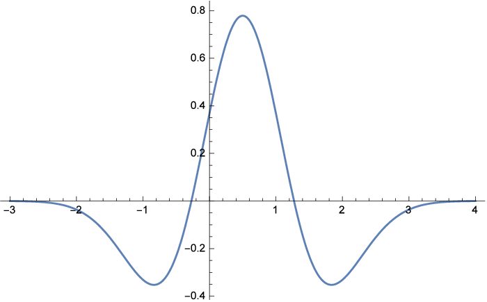
The interaction function in Eq. (2.3) is defined by
| (2.4) |
This Gaussian term expresses the effect of the difference between the strength of the love between two agents. This term notices some life reality. the interaction function is the largest if the strength of the lover and that of are similar, while if the strengths are quite different, - though not neglected.
The parameter is positive and scales the intensity distribution of the ”lover strengths”. For simplicity, we assume .
The parameter can be considered as an element of a matrix which specifies various scenarios on the types of lover’s interactions.
Here we define four different -matrices each of which characterizes different love scenarios among three lovers , and . The possible -matrices for describing one-way love are
| (2.5) |
represent a situation that is not interested in and , but and care about and wish as a lover. This can be imagined as a situation in which two individuals fall in love with a (famous) person, - who a priori does not care.
In contrast, expresses that falls in love with both and , but and do not care about .
We also describe a famous situation in relationships called ”love triangle”. Two main forms of love triangle have to be distinguished: there is the rivalrous triangle, where the lover is competing with a rival for the love of the desired, and the split-object triangle, where a lover has split some attention between two love objects”.
Thus, we consider is interested in both and , and also and care about and wish love; and do not ”know” each other, such that there is no interaction between and . The possible -matrix for expressing such a love triangle game is
| (2.6) |
In contrast, one may consider a situation in which does not like and and also and distaste . (An analogy for this scenario is the case where a country has a conflict with two other countries which they are neither allied nor hostile.) The possible -matrix for expressing this kind of interaction is
| (2.7) |
2.1 Fixed point analysis & stability
To access to all possible states and systems’ evolving states, it is useful to find the phase space of the parameters in the dynamical equations. The phase space trajectory represents the set of states compatible with starting from any initial condition. The dynamics equations could be represented as a vector field in the space ; the points of these vector space are:
| (2.8) |
Each point of space evolves in time from to .
| (2.9) |
This evolution path draws a trajectory in the space ; each vector shows the ”speed” and the evolving direction in this space.
In order to investigate the dynamics of the system, a fixed point analysis can be fruitful. A fixed point of a function is a point which is mapped to itself by the function. In other words, the evolution of the equations stops at the fixed points, thus the time derivative in the evolution equations is equal to zero. At the fixed point , each component of the vector field vanishes. The fixed points are found by solving Eqs. (2.10):
| (2.10) |
A fixed point is stable if the trajectory of all points in the vicinity of the fixed point tends to evolve toward the fixed point. These points are called attractors or sinks. A fixed point is called repeller or source if all the points in the vicinity of the fixed point flow away or diverge from the fixed point; it is called a saddle point if the vicinity of the fixed point converges to the fixed point along some directions and diverges along other directions [13].
If the derivative of the vector field along a specified direction at the fixed point is positive, the fixed point is an attractor along this direction; if it is negative, the fixed point is a repeller along that direction. Numerically or analytically,
| (2.11) |
| (2.12) |
Using the first order coefficient of the expansion, the Jacobian matrix is
| (2.13) |
One can probe the stability of a fixed point by evaluating the eigenvalues and eigenvectors of the Jacobian matrix computed at each corresponding fixed point.
| (2.14) |
In the above equation, is the i-th eigenvector and is the corresponding eigenvalue. The fixed point is an attractor along an eigenvector if the corresponding eigenvalue is negative; it is a repeller if the eigenvalue is positive; when all the eigenvalues are negative, the fixed point is an attractor and vice versa; if there are both negative and positive eigenvalues, the fixed point is a saddle point [13].
3 RESULTS
The dynamics equations are usefully rewritten as
| (3.1) |
| (3.2) |
| (3.3) |
In the following, we solve the equations for each .
3.1 One-way love type
| (3.4) |
1. is a trivial fixed point of the system. It is unstable, the eigenvalues of the Jacobian matrix are positive .
2. is an attractor fixed point; its eigenvalues are . The corresponding eigenvectors are , and .
3. is a saddle point with the eigenvalues ; the corresponding eigenvectors are , and . It is an attractor along vector and repeller along two other directions and , so all the points on the axis end up to this point; see Fig. 1.
4. is similar to the point due to the symmetry of the evolution equations; it is a saddle point; its eigenvalues are ; the eigenvectors are , and . All the points along the direction converge to , whence the basin of attraction for this fixed point is the axis ; see Fig. 2
5. There is a line of fixed points in the plane . All the points on the line are fixed point and the eigenvalues are:
| (3.5) |


The eigenvalue is greater than 0 in the region , as shown on Fig. 3; whence these points are unstable and saddle points. The eigenvector corresponding to the eigenvalue is and therefore all the points in the plane converge to this line along the direction ; Fig. 4.
The results are summarized in Table 2
| Fixed Point | Stability | Basin of attraction |
|---|---|---|
| repeller | - | |
| attractor | Global | |
| saddle | Axis | |
| saddle | Axis | |
| The line | saddle | The surface |

In this case, the vector field is perpendicular to the normal vector of the surface ; thus, the field is tangent to this surface and the trajectory remains on this surface forever and converges to the fixed point for all the initial values. This means that if the two lovers and were initially and equally interested in , their amount of love remains equal for ever. On the other hand, if none of and are interested in , their amount of initial love, decreases and converges to zero; this is in contrast to the love of which increases and goes to the full capacity. When the strength of the love interaction between and the two lovers , is equal, no one can win the love competition.
The point is the only stable fixed point; all the points in the space except those on the plane converge to this point. This result seems intuitive. As the two lovers are not interested in at all, cannot impress them but as is fascinated by both and the amount of its love increases; it will end up to be deeply in love with both and .
We also find an interesting situation when the lover starts with a little love at the beginning of the game and when the lovers and get somehow interested in ; both demand more attention from the lover ; therefore their love increases at first but later they become less interested and their love decreases, ending up to zero; see Fig. 5. This case occurs when the initial is small and for ; in such a case, and . One can numerically find a region in which and increase at first; see Fig. 6.
On the surface , there is a line of fixed points; the basin of attraction is the surface ; this means that if the lover wishes neither nor at first it will remain uninterested, but there will be a competition between and to obtain ’s attention; the initial ratio of their love remains unchanged and their interest reaches a balance state on the line ; see Fig. 4 again.


3.2 One-way love type
| (3.6) |
The fixed points, stability regimes, and basins of attraction are summarized in Table 2.
1. is an unstable fixed point and its eigenvalues are ;
2. is a saddle point with eigenvalues . The eigenvector corresponding to the eigenvalue is ; thus, it is an attractor along the axis ;
3. is a stable fixed point: the eigenvalues are ; the corresponding eigenvectors are , and ; see Fig. 7;
4. is similar to the point ; thus, it is a stable fixed point; he eigenvalues are ; the corresponding eigenvectors are , and ;
5. There is a line of fixed points in the plane . All the points on the line are fixed points; their eigenvalues are:
| (3.7) |
The eigenvalue is negative in the region , so that these points are stable and attractors. The eigenvector corresponding to the eigenvalue is ; therefore all the points in the plane converge to this line along the direction ; see Fig. 8.
| Fixed Point | Stability | Basin of attraction |
|---|---|---|
| repeller | - | |
| saddle | Axis | |
| stable | The surface | |
| stable | The surface | |
| The line | stable | Global |


All the points in the space except the axis converge to this line. This result seems intuitive, as is not interested in and at all, cannot be impressed by the lovers and . But as and are fascinated by the amount of their love increases up to be deeply in love with forever.
When the initial love of the lovers and is small and under the condition with , the lover gets somehow interested in and and demands more attention from these lovers; whence its love increases at first. As an example consider a movie star at the beginning of its work when he or she is not a celebrated person and is known by a few people, the movie star is interested in getting fans and greedily demands their attention. But later on, looses to be interested; thereafter decreases and ends up at zero; see Fig. 9. One can numerically find a region in which increases at first; Fig. 10.
Just like in the previous section, one finds the vector field to be tangent to the surface ; all the trajectories remain on this surface forever and converge to the fixed point .


3.3 Love triangle type
| (3.8) |

1. is a trivial fixed point of the system. It is unstable, the eigenvalues of the Jacobian matrix are positive .
2. There are three fixed points on the surface . , , ; is an attractor fixed point; its eigenvalues are .
The eigenvalues of the point are ; thus it is a saddle point. The eigenvector corresponding to is . Therefore, it is an attractor along the axis . On the other hand, it is a repeller along the two directions and ; Fig. 12.
Similarly, the point is a saddle point with the eigenvalues . The eigenvector corresponding to is . Therefore, it is an attractor along the axis .

3. There are two other fixed points , on the plane.
The fixed point is similar to the fixed point and its eigenvalues are the same ; thus, it is an attractor fixed point.
The eigenvalues of the point are . The eigenvector corresponding to is . So this point is a saddle point which attracts along the axis ; see Fig. 13.

4. There exists a line of fixed points in the plane . In other words, all the points on the line are fixed points. These points are saddle points and their eigenvalues are:
| (3.9) |
Since , the eigenvalue is greater than 0 in this interval, so these points are saddle points. The eigenvector corresponding to is and is located in the plane ; thus, all the points in this plane converge to the line of fixed points; see Fig. 14.

5. The fixed point is an unstable saddle point. Indeed, the eigenvalues are ; the corresponding eigenvectors are:
| (3.10) |
| (3.11) |
| (3.12) |
This point is a repeller along the third eigenvector with eigenvalue . Thus, all the trajectories perpendicular to this vector at this point will not be repelled. The surface is perpendicular to the vector ; the inner product of vector field lies on the surface ; the normal vector to the surface is zero:
| (3.13) |
Therefore, all the trajectories on the surface remain on this surface and converge to the fixed point . Thus, the surface is the basin of attraction of this point and all the trajectories on this surface converge to the fixed point ; Fig15.
The trajectories which are not on the surface diverge from the surface. The points that are located under this surface converge to the stable fixed point (Fig. 16); the points that are located above this surface converge to the fixed point ; see Fig. 17.
The results are summarized in Table 3.


So, two fixed points and correspond to a situation in which one of the lovers wins the love game in a love triangle and can get all the attention of the lover ; if one of the lovers and is initially more interested in , it will capture the full attention of the lover .
But if the two lovers love equally at first, no one wins the game and both share the love and attention of , - and reach the point . As this fixed point is strongly unstable and if the condition changes a little bit, the love path diverges from the point . For example, if the love of regresses and gets lower than , then will loose the game and the love path ends up in .
| Fixed Point | Stability | Basin of attraction |
|---|---|---|
| repeller | - | |
| attractor | ||
| saddle | Axis | |
| saddle | Axis | |
| attractor | ||
| saddle | Axis | |
| saddle | The surface | |
| The line | saddle | The surface |
3.4 Love triangle type
Now consider:
| (3.14) |

In this case the fixed points and their stability quite differ from the previous case. The three surfaces , and are illustrated in Fig. 18.
1. The point is an unstable fixed point with eigenvalues .
2. There are three fixed points on the plane . The point with the eigenvalues is an unstable saddle point. It is attractor along with the eigenvalue , as shown in Fig. 19. The point is an attractor fixed point and its eigenvalues are . The point with eigenvalues is an attractor.

3. There are two other fixed points on the plane . The point with eigenvalues is an unstable saddle point. All the points along the eigenvector converge to this point; see Fig. 20. The point with eigenvalues is an attractor.

4. There is a line of fixed points in the plane . All the points on the line are fixed points with eigenvalues:
| (3.15) |
The third eigenvector is negative in the region . So, unlike in the previous case, all the fixed points on this line are stable: Fig. 21.

5. In the region , there is a fixed point which is an unstable saddle point; its eigenvalues are . Consider the surface . The normal vector of this surface is The vector field on this surface is:
| (3.16) |
| (3.17) |
| (3.18) |
The inner product of vector field on the surface and the normal vector to the surface, , is zero.
| (3.19) |
Therefore, the vector field is perpendicular to ; thus, the vector field is tangent to the surface and all the trajectories remain on this surface. These trajectories converge to . The trajectories initially located under the surface converge to the stable fixed point (see Fig. 22); those located above the surface converge to the line ; see Fig. 23.
As an example for this case of interaction, consider three countries , and . There is a hostility between the country and the two countries and but there is no any hostility or alliance between the countries and .
The point corresponds to a situation in which is interested in the two others and demands a good relationship, but and are not interested in and tend to boycott it.
As mentioned before there is a fixed point on the surface for which the basin of attraction is . This means that under this special condition, there is an unusual fixed point in which all the countries/lovers are interested in each other and seek a mutually peaceful relationship, like a ”menage a 3”. However, this balanced state is extremely unstable; any small deviation (perturbation) from the surface, gives rise to a divergent trajectory from the fixed point, either leading to the fixed point or to the line .
(A ”symmetric solution” is possible: the line turns out to be obviously the opposite of this previously discussed situation.)


The results are summarized in Table 4.
| Fixed Point | Stability | Basin of attraction |
|---|---|---|
| repeller | - | |
| saddle | ||
| attractor | ||
| attractor | ||
| saddle | ||
| attractor | ||
| saddle | The surface | |
| The line | attractor |
4 CONCLUSIONS
In this paper, we have tried to describe one of the most mysterious aspects of a human life, love, in terms of complex system theories and nonlinear dynamics. We have used the Verhulst-Lotka-Volterra prey-predator model in order to take into account competitive or cooperative attitudes between ”agents”. We have considered 3 agents (”lovers”) for establishing the minimal complexity set of non linear differential equations, and have introduced different interaction matrices in order to mimick some (well-known) situations in a 3 partner love story game. We have tried to answer some questions, like: What is the end of a love story in different scenarios? Under which condition will occur different situations? Which ones of these final situations are stable and under which conditions?
In this love triangle, we have further reduced the number of scenarios, only considering that there is no direct interaction (love or hate) between the lovers and , yet keeping in relation with both neighboring partners. Therefore, most of the time one of the rivals wins the love game and the other one will be completely ignored. However under some conditions, as outlined in the main text, the game does not necessarily have any ”winner”; there is a possible stable trio of lovers. Interestingly, this situation is very sensitive and is not stable. This means that it is hard to love several persons simultaneously, - in this kind of model.
We have also considered the opposite of the previous love triangle case, that is is not interested in and . As an example for this case consider the political relationship among three countries which are hostile together. We argued that in this case, in spite of the unfriendly direct interaction between the agents, there is always some agent looking for a friendly relationship; under special conditions, described in the previous sections, everybody demands friendly relationship with the others. But this situation is again not stable. We have discussed two different scenarios in this so called ”one-way love”. In the first scenario, the central lover is interested by the two agents and but these do not love (care about) . The second scenario is the opposite: the two lovers and love , but the agent is not interested in them. The analogy with ”public stars” or ”celebrity” has been mentioned in the main text.
In the first scenario, will eventually be deeply in love with the two others, but these two will not be fond of . Under special conditions in which starts the love game from a low amount of interest, the two agents and get somehow interested in the central lover ; it seems they are appealing for more love and attention from the lover at the beginning of their love journey.
In the second scenario of one-way love, will not be in love with the two other lovers, but these two lovers reach a balance point due to their competition in loving . Just like in the first scenario, if the lovers and start the love game from a low amount of interest, the central agent will be interested in them and be looking for more love and attention, right from the beginning of the love journey.
In our analysis, we have supposed that the strength of the interaction is a binary variable, whatever the couples, and is time modulated in a self-organized, symmetric, and preferential way through some Gaussian strength weight; we have also supposed that the interaction term between and can be neglected. In order to achieve a deeper understanding it can be fruitful to reconsider these constraints in future research. It seems that it would be useful also to think about the evolution of love under ”external fields”, and about the dynamics of the system over time, allowing for memory effects [14, 15, 16].
References
- [1] S.N. Dorogovtsev and J.F.F. Mendes, Evolution of Networks: From Biological Nets to the Internet and WWW. (Oxford University Press, Oxford, 2003).
- [2] A. Rapoport and A.M. Chammah, Prisoner’s Dilemma: A Study in Conflict and Cooperation (University of Michigan Press, 1965).
- [3] W. Poundstone, Prisoner’s Dilemma. (Doubleday, 1992).
- [4] V. Volterra, Variazioni e fluttuazioni del numero d’individui in specie animali conviventi, Mem. R. Accad. Naz. dei Lincei VI, 2, 31 (1926).
- [5] N. K. Vitanov, Z. I. Dimitrova, and M. Ausloos, Verhulst-Lotka-Volterra (VLV) model of ideological struggle, Physica A 389, 4970 (2010).
- [6] N. K. Vitanov, M. Ausloos, and G. Rotundo, Discrete model of ideological struggle accounting for migration, Adv. Compl. Syst., 15, Suppl.1, 1250049 (2012).
- [7] P. F. Verhulst, Recherches mathématiques sur la loi d’accroissement de la population, Nouv. Mémoires de l’Académie Royale des Sci. et Belles-Lettres de Bruxelles 18, 14 (1845).
- [8] P. F. Verhulst, Deuxième mémoire sur la loi d’accroissement de la population, Mémoires de l’Académie Royale des Sci., des Lettres et des Beaux-Arts de Belgique 20, 1 (1847).
- [9] L.F. Caram, C.F. Caiafa, A.N. Proto, and M. Ausloos, Dynamic Peer-to-Peer Competition, Physica A 389, 2628 (2010) .
- [10] L.F. Caram, C.F. Caiafa, A.N. Proto, and M. Ausloos, Cooperative peer-to-peer multiagent based systems, Phys. Rev. E 92, 022805 (2015).
- [11] A. Sonubi, A. Arcagni, S. Stefani, and M. Ausloos, Peer to Peer Multiagent Competition and Cooperation with Network Effect, Physical Review E 94, 022303 (2016).
- [12] A. Gadomski, M. Ausloos, and T. Casey, On Dynamical Systems Theory in Quantitative Psychology and Cognition Science: A Fair Discrimination Between Deterministic and Statistical Counterparts is Required, Nonlinear Dynamics, Psychology, and Life Sciences 21, 129 (2017).
- [13] S.H. Strogatz, Nonlinear dynamics and chaos: with applications to physics, biology, chemistry, and engineering. (Westview Press, 2014).
- [14] H. Safdari, M. Kamali, A. Shirazi, M. Khalighi, G.R. Jafari, and M. Ausloos, Fractional Dynamics of Network Growth Constrained by Aging Node Interactions, PLoS ONE 11, e0154983 (2016)..
- [15] F. Hassanibesheli, L. Hedayatifar, H. Safdari, M. Ausloos, and G.R. Jafari, Glassy states of aging social networks, Entropy 19 246 (2017) .
- [16] M. Saeedian, M. Khalighi, N. Azimi-Tafreshi, G.R. Jafari, and M. Ausloos, Memory effects on epidemic evolution: The susceptible-infected-recovered epidemic model, Phys. Rev. E 95, 022409 (2017).