Constrained Density Functional Theory Calculation with Iterative Optimization
Abstract
An iterative optimization approach that simultaneously minimizes the energy and optimizes the Lagrange multipliers enforcing desired constraints is presented. The method is tested on previously established benchmark systems and it is proved to be efficient and accurate. The approach can also be efficiently used when the constraint is not a scalar quantity but a spatially varying function like the charge density distribution.
I Introduction
Density functional theory (DFT) [1] is one of the most important approaches to calculating ground state properties in molecules and solids. The extension of DFT for ground state calculations in constrained systems (cDFT) [2, 3] opened a new venue for the description of charge excitations [4], magnetic transitions [5], spin dynamics [6] and electron transfer [7]. This technique became a more powerful tool with a greatly enhanced range of applicability through the introduction of a self-consistent formulation by Wu and Van Voorhis [8]. It is now implemented in many computer codes using localized basis sets (NWChem [8], QChem [9, 10], SIESTA [11], deMon2k [12], ADF [13]), plane waves (CPMD [14], QuantumESPRESSO [15], VASP [16]), density matrices (CONQUEST [17]), wavelets (BigDFT [18]), and projector augmented wave (PAW) methods [19].
Armed with these powerful computational tools the cDFT has been intensively used (see a recent review in Ref. [20]) in a wide variety of problems including electron transfer reactions [21, 22, 23, 24, 25], excitation energy transfers [26], calculation of coupling parameters [27], and non-collinear magnetism [16]. Computational approaches using local constraints [28], orthogonality conditions [29], and constrained-orbitals [30] have also been developed.
In the direct optimization approach of Wu and Van Voorhis [8], a constraint is added to the energy functional using the Lagrange multiplier method. The Lagrange multiplier determines the constraining potential but it is not explicitly known. Wu and Van Voorhis have shown that the functional is a strictly concave function of the Lagrange multiplier and there is a unique stationary point which is a maximum. They proposed a nested loop approach with an outer self-consistent loop (a normal DFT loop) and an inner constraint loop. The constraint loop determines the Lagrange multiplier aided by the first and the second derivatives of the functional. The constraint iterations are relatively cheap using localized orbitals (the cost is a diagonalization of the Hamiltonian), but in the case of plane wave or real space grid codes describing larger systems, this step can be a bottleneck.
In this paper we implement an approach that simultaneously minimizes the energy and optimizes the Lagrange multipliers to satisfy the constraints. The method uses steepest descent iteration for the orbitals and the Lagrange multiplier is iteratively updated in each step. The Lagrange multiplier is adjusted in each iteration in order to enforce the constraining condition [31, 32] on the desired expectation value. The advantage of the approach is that it can be easily implemented alongside steepest descent or conjugate gradient minimization allowing efficient cDFT calculations using real space grids. A distinctive merit of the method is that it can also be used to enforce spatially varying constraints. One can constrain not only a prescribed total charge in a region, but a desired density distribution can also enforced opening new possible applications for cDFT.
In section II, we outline the main points of the formalism, leaving the details collected in the Appendices. In section III, numerical tests will be presented. The last section is a short summary. Two appendices are added to describe the iterative diagonalization formalism, to overview of Lagrange multiplier approach, and to motivate the iterative optimization.
II Formalism
II.1 Constrained Density Functional Theory
In DFT the total energy in atomic units (a.u.) is given by
| (1) |
where
| (2) |
is the kinetic energy, is the Coulomb energy, is the exchange-correlation energy, is the external potential, and
| (3) |
is the electronic density for spin of electrons (). A generic constraint can be defined as
| (4) |
where is an operator and is a desired expectation value. For example, it is very common to constrain the charge density so that there is a specified number of electrons for each spin, , within a certain region of space:
| (5) |
Here, is a weighting function confining the electron density into a specified spatial region (e.g. is equal to 1 within a certain volume and 0 elsewhere).
In order to minimize the total energy of Eq. 1 subject to the constraint of Eq. 4, a functional is defined to be
| (6) |
where is the Lagrange multiplier.
Minimizing with respect to forces the constraint to be satisfied. By making this functional stationary under the condition that the Kohn-Sham orbitals are orthonormalized (see Appendix B and the discussion in Ref. [33]), one gets the Kohn-Sham equations with an extra term, the constraining potential ,
| (7) |
Here,
| (8) |
where is the exchange and correlation potential. Up until now, the popular notation of the literature has been followed; however, from now on, we drop the spin index for simplicity and assume that each orbital is doubly occupied.
For a given , one can determine the orbitals, and with the correct the constraint is fulfilled. Wu and Van Voorhis [8] have established a means of solving for a unique stationary point. They have shown that is a strictly concave function of , with only one stationary point which is a maximum. Both the first and second derivatives of with respect to can be derived, so the optimization can be done efficiently. Finding requires the solution of Eq. (7) for a given lambda and updating lambda, thus optimizing (see Appendix B.2). The desired constraining potential is found when the constraining equation is satisfied with respect to a prescribed accuracy. Further discussion on the optimization of constrained DFT can be found in Ref. [33], in which efficient calculations involving multiple constraints are described.
II.2 Iterative minimization
We will use a method that is based on iterative diagonalization. This approach is often used in cases of large basis dimension, such as for the three-dimensional real space grid representation, where direct diagonalization of the Hamiltonian matrix is infeasible and alternate methods must be used to determine the lowest energy eigensolutions. The simplest approach is a steepest descent iteration
| (9) |
Here, ,
| (10) |
and indicates Gram–Schmidt orthonormalization, required to preserve the orthonormality of the single-particle states at each update step. The starting wave function, , is some initial guess, e.g. linear combination of atomic orbitals, and is chosen to be sufficiently small for convergence. The steepest descent step can be derived from imaginary time propagation and can be improved by using higher order approximations to the exponential operator (see Appendix A).
II.3 Iterative minimization with a constraint
The advantage of the iterative diagonalization is that it can be combined with a step which is designed to enforce the constraints. The motivation for the concrete form of the iterative updates, the possible implementations, and the highlights of earlier works is summarized in Appendix B.
In the case of constraint, the goal is to update each orbital towards the minimum energy configuration while maintaining that an arbitrary expectation value, related to an associated operator, , does not change from one static iteration to the next; i.e.
| (11) |
Furthermore, the value of this expectation value is meant to match a given input value,
| (12) |
These conditions may be incorporated into the above iterative formalism by the inclusion of a Lagrange multiplier constraint term such that the new update scheme becomes
| (13) |
In this new update scheme, one has to simultaneously iterate the Lagrange multiplier . The simplest choice is to use a steepest descent iteration for as well (see Appendix B.3), but one can work out a much better scheme by choosing in such a way that the the constraint in Eq. (11) is satisfied.
To this end [31, 32], one includes an intermediate step
| (14) |
The difference of the relevant expectation value between the original and half steps is calculated,
| (15) |
so that the Lagrange multiplier may be updated as
| (16) | |||||
Here, and are numeric constants; their role is explained in Appendix B.4. A good choice for is a value between 0.9 and 1.0, and that for is around . In the above equation, is corrected with two terms. The first correction seeks to preserve the expectation value of by reducing the change in (see Eq. (62)). The second correction term adjusts the expectation value toward the desired value (see Eq. (61)).
With these readjustments, the th step is given as
| (17) |
This update step can be considered as a simultaneous correction meant to preserve the expectation value as well as force the expectation value to be equal to a desired quantity. The numerical constants appearing in the iteration play a similar role to the density mixing parameters in the self-consistent solution of the Kohn-Sham equations by helping the speed of convergence. The motivation and details of the above steps for the simultaneous diagonalization of the Hamiltonian and the optimization of is given in Appendix B.4.
This update scheme settles the Kohn–Sham system into the minimum energy state while maintaining a constraint on an arbitrary state expectation value. Effectively, what occurs is the convergence of the Kohn–Sham system towards the global ground state for a total effective potential which is iteratively updated simultaneous to the orbitals. Thus, the final state may be fully constructed by real-valued orbitals, and the converged Lagrange multiplier term, , represents a fictitious, additional external potential which corresponds to a Kohn–Sham state exhibiting the desired expectation value.
III Results
In this section we present results of the iterative constraint update scheme. In each case, a real space grid representation was used alongside a finite difference representation of the kinetic energy. The ion cores were treated using norm-conserving Troullier and Martins pseudopotentials [34].
III.1 Simple model system
As a simple numerical test we consider a three dimensional harmonic oscillator (a.u.) with =5 orbitals, subject to the constraint
| (18) |
where
| (19) |
In the test calculation, the parameters and are chosen to be 1 and 25 a.u., respectively. The model is analytically solvable. Adding the term to the Hamiltonian is equivalent to a modified harmonic oscillator potential with . The square radius of a harmonic oscillator wave function with quantum numbers is equal to , so the condition determines the analytical value of and the energy. The numerical solution for a simple steepest descent update and the optimization approach presented in the previous section is compared in Fig. 1. The figure shows that the optimization is very accurate, both in energy and in constraining , and the convergence is very fast. The steepest descent approach, based on Eqs. (54) and (55), also works but the accuracy is orders of magnitudes worse. This simple but clean example (no self consistency) shows that the optimization approach is accurate and fast.

III.2 Charge constraint
Now we apply the iterative optimization scheme to charge transfer systems studied by Wu and Van Voorhis [8, 22]. They used a weight function, , which designates coordinate space belonging to the donor with a value of 1 and that of the acceptor with a value of -1. In this way, a Lagrange multiplier term is added to the Kohn–Sham equation as , effectively representing a step potential which may be tuned during optimization until the desired charge imbalance between the two partitions,
| (20) |
is reached. The weight function may be defined using a scheme such as Hirshfeld partitioning [35, 36] such that
| (21) |
where represents the unperturbed electron density of ion and is its location.
In our formalism, the weight function may be chosen as the operator whose associated expectation value, , is being constrained to a given value. In this way, charge constraint optimization may be performed in DFT using a real space grid approach which, unlike the atomic orbitals basis, does not allow for a practical means of storing the full Hamiltonian matrix and, instead, relies on algorithms which describe the action of the Hamiltonian matrix on a wave function vector. Furthermore, in this update scheme, one is not required to use a nested-loop form in which either the energy minimization or the constraint condition is satisfied via an inner loop while the other is satisfied using the outer loop. In the iterative constraint method, one progresses towards the stationary point by simultaneously updating each. This may lead to significantly faster runtimes or enhanced stability.
Of the simplest cases to consider is the diatomic molecule. Here, one atom is designated as the donor, and the other is the acceptor. The above described procedure was carried out for a desired charge difference between the two atoms of electrons. The width of the computational box was 6 Angstroms on each side with 25 grid points along each axis. A plot of the convergence of and of the Lagrange multiplier, , is presented in Fig. 2. We find that only a small number of iterations are needed for satisfactory convergence in this case. The resulting value for , indicating the depth of the step potential enforcing the charge difference, was -27.01 eV. The electron density for the molecule using conventional DFT is shown in Fig. 3(a) and that of the charge constrained molecule is shown in Fig. 3(b). By including an additional potential of in a conventional DFT calculation of the molecule, the charge difference of electrons naturally arises and the density, shown in Fig 3(c), nearly exactly matches that of the constrained DFT case.

(a) (b) (c)



The present approach and that of Wu and Van Voorhis is compared in Fig. 2. The present approach converges much faster for , after about 20 iterations the value of is accurate up to 5-6 digits. More importantly, also converges faster using the optimized iteration, despite the fact that it’s value is adjusted to enforce the constraint. To compare the computational burden, we note that each self consistent loop was updated in the same way for both approaches. The computational cost difference comes from the fact that the Wu and Van Voorhis method is using an internal loop (see Appendix B.2) which requires 3-4 additional operations per iteration than in our implementation. Thus the computational cost of the Wu and Van Voorhis approach is about 3-4 times higher than that of the present one for the same number of self-consistent energy minimization iterations.
This comparison is meant to highlight the potential efficiency of the present method, but it is not a strict comparison of the computational cost. Using the two approaches for different systems or using different basis functions might result in different computational efficiencies. Calculations using localized basis functions with small Hamiltonian matrices would most definitely be faster using the method of Wu and Van Voorhis. The second derivate (see Appendix B.2) of the functional would also increase the convergence, but that is not readily available in real space calculations.
We next consider the small systems tested by Wu and Van Voorhis in Table 1 of Ref. 22. For long separation distances between the donor and acceptor molecules, , one would expect that the energy varies as . A good test of the energies calculated by a charge constraint DFT program would be to plot the total energy vs. and show the expected linear dependence. Furthermore, one may use the slope of this curve in order to determine the total energy of the charge-separated (CS) system; i.e. . Being that at an infinite separation distance, the two molecules should be independent of one another, this total energy should equal the sum of separate calculations for the appropriately ionized donor and acceptor molecules, that is and in the case of .
An example trend of the total energy vs. is presented in Fig. 4 for the system – and a charge difference of . The data is well fit by a linear trend line. The slope indicates an expected CS total energy of -1069.735 eV. This value is in good agreement with the total energy of separate calculations for the and molecules, being -1070.970 eV. These values, as well as those for the cases of – and –, are presented in Table 1. We note that each value for is higher than its counterpart by about 1.15 eV. Apart from this small systematic shift, all values agree well, indicating that these long-range charge transfer states are being well-represented by the present scheme. We note that the reported values in Table 1 do not represent total energies of these systems. This is due to the fact that pseudopotentials have been employed, and the frozen-core approximation energies, corresponding to the pseudopotential contributions, have been neglected. In principle, because the difference in total energy is nearly always the desired calculated quantity, one may compare such valence energies among like systems, represented using the same pseudopotentials, as if they were the true total energies.

| D | A | % diff. | ||
|---|---|---|---|---|
| -1069.735 | -1070.970 | 0.115 | ||
| -1767.172 | -1768.204 | 0.058 | ||
| -3323.066 | -3324.250 | 0.036 |
Finally, we investigate the popular charge transfer excitation in zincbacteriochlorin-bacteriochlorin (ZnBC–BC). This system is a common component of suggested light harvesting devices, appearing with a phenylene link. However, it has been demonstrated that ignoring the link introduces negligible error [37]; therefore, the pair of isolated molecules separated by 5.84 Å is commonly studied. The charge transfer excited state of this complex was of the earliest shown to be misrepresented by time-dependent density functional theory (TDDFT) [37], due to an incorrect treatment of the long-range exchange potential. Thus, there are many studies devoted to the correction of this shortcoming. Such calculations include TDDFT using various local [37, 38, 39] and hybrid [39] functionals, methods combining a configuration interaction singles (CIS) approach [37, 40], and also use of the Bethe–Salpeter formalism [41]. The CDFT formalism of Wu and Voorhis was also initially applied to this system [8, 22], there using an atomic orbitals basis, specifically the basis set, and the Becke–Lee–Yang–Par (BLYP) functional [42, 43]. This approach has also been recently tested on the ZnBC-BC complex using a flexible Daubechies wavelet basis and the LDA functional [44].
(a)

(b)

The difference of the DFT-calculated ground state density for ZnBC–BC and the charge constrained DFT density is shown in Fig. 5(a) and Fig. 5(b) for the cases of – and –, respectively. The LDA relaxed coordinates were provided by Ratcliff et al. of Ref. 44. The energy values for this large system maintain a linear dependence with regards to , as shown in Fig. 6. The energies of the two excited states relative to the neutral ground state, using a separation distance of Å, were determined to be 3.54 eV for – and 3.95 eV for –. The latter value agrees well with previously calculated values (3.91 eV [37], 3.94 eV [8], and 3.98 eV [44]) while the former is lower than similar studies (3.71 eV [37], 3.75 eV [44], and 3.79 eV [8]). The difference between the results comes from several sources. The present code uses pseudopotentials and LDA with real space grid representation, while the calculations in Refs. [8, 37] are based on all-electron codes with the BLYP functional. The computation in Ref. [44] is also based on LDA but uses Daubechies wavelets, significantly reducing the effect of the coarseness of the real space grid (e.g. eggbox effect). The most important source of the difference is that in our real space grid approach the weight function is not represented in the same way as in the other approaches using the Voronoi grid [45] or wavelets.
III.3 Density constraint
The approach can be extended to more general constraints as well. In this section we demonstrate the ability of the present approach to constrain the spatial density, requiring that is equal to a given value, . In this case, the operator becomes the density operator such that
| (22) |
and
| (23) |
Given a desired initial density distribution, , and using the steps defined in Eqs. (14), (16), and (17), one looks for the potential, , which generates the Kohn-Sham orbitals, , so that
| (24) |
As a first example, we use a simple system, the H2 molecule. Fixing the protons at 0.74 Å apart, the two-electron Coulomb problem can be solved very accurately using the variational method with explicitly correlated Gaussian basis functions [46]. The calculated “exact” electron density, shown in Fig. 7, will be the target density . Fig. 7 compares to the density obtained by a conventional DFT calculation. The two densities differ mostly in the middle region between the two protons where the DFT density is higher. Using the density constraint, we then instruct the DFT density to be equal to . The asymptotic fall of the density is also different, but that is not so important for this test case. The cDFT calculation constrains the density to satisfy , and the constrained and exact densities are indistinguishable in Fig. 7. The cDFT potential (the Kohn-Sham potential plus ) and the DFT potential are compared in Fig. 7. The main difference is that the cDFT potential is higher in the middle region, pushing out the charge and correcting the difference between the exact and DFT result. In principle, calculations like this can be used to improve exchange-correlation potentials if accurate densities are available. To check the calculation, one can use the resulting and add it to the Kohn-Sham Hamiltonian as an external potential. The self-consistent solution produces the desired density distribution .
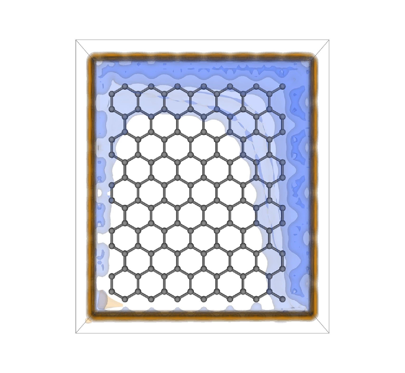
The next example demonstrates that the approach works for larger systems as well. In this case, we calculate the electron density of a graphene sheet in a periodic supercell calculation. Taking this density, Fig. 8(a), we use a masking function to gradually decrease the density to zero at the boundaries, Fig. 8(b), and use this distribution as .
The cDFT is now used in conjunction with a system of the same molecular geometry as the supercell but with the outer perimeter of carbon atoms removed. Extra Kohn–Sham orbitals are added, beyond those corresponding to the to carbon atoms, in order to ensure that the number of electrons of the initial non-converged density matches that of . We note that there will be one orbital of non-integer occupation. The cDFT generates , Fig. 8(c), so that yields as the ground state density. The calculation of a converged constraining potential needs about two to three times more iterations than a conventional DFT iteration. The calculated can be checked by using it as an external potential to produce .
This example serves to show that the approach is applicable and converges for larger systems as well. One can recognize the formation of potential wells within the shape of near the perimeter of the graphene fragment which correspond to the carbon atoms missing in the input molecular geometry. In principle this graphene fragment can be used to study defects without the problem of periodic images, but still keeping the proper density. One can also use the approach to embed a smaller system into a larger system with density constrains at the boundary. In Ref. [47] charge densities in a boundary region between the two domains has been connected using cDFT to facilitate multiscale calculations using a single scalar Lagrange multiplier. The present approach offers a more flexible embedding possibility.


IV Conclusion
We have implemented an iterative optimization approach for constrained density functional calculations. In this approach the energy minimization and the optimization of the Lagrange multipliers enforcing the constraint is simultaneously iterated. The ideal Lagrange multipliers are determined by enforcing the constraint on the Kohn-Sham orbitals at each self consistent iteration steps.
The accuracy and efficiency of the present approach is demonstrated on previously studied systems. Comparing the computational cost to previous methods based on the direct optimization of the Lagrange multiplier [8], the present approach is expected to be competitive. In the case of real space grid basis approaches, the present method is definitely favorable, by a 2-3 times savings in computational cost.
The method is not limited to charge constraints where only a single (or a small set of) Lagrange multiplier is optimized. We have shown that one can prescribe a general, spatially varying density, and the external potential that generates this density as a ground state can be calculated. The applicability of this approach to calculate a spatially dependent Lagrange multiplier may open up possibilities of embedding smaller systems into larger systems, prescribing boundary conditions using density, or enforcing orthogonality to a given ground state.
Acknowledgement: The work of A. S. Umar was supported by DOE grant No. DE-SC0013847.
Appendix A Imaginary time propagation
In this appendix, for completeness of the presentation, we show how the popular steepest descent iteration can be derived from the imaginary time step propagation [48]. The important part of this step is that although we only used, to lowest order, the simplest iteration, systematic improvement is possible by including higher order terms. The origin of the imaginary time propagation name comes from the similarity of each optimization step and the solution to the time-dependent Kohn–Sham equation,
| (25) |
for short time steps, :
| (26) |
For imaginary time step propagation, one makes the transformation and introduces the parameter such that the procedure takes the form
| (27) |
Here, we have replaced the notation of our employed wave functions so that they now represent arbitrary functions which are iteratively being updated and approaching the ground state eigenfunctions of . This is seen by noting that such an arbitrary function at iteration , , may be expanded as a linear combination of the eigenfunctions of :
| (28) |
By plugging this expansion into Eq. (27), one obtains
| (29) |
and notes that repeated action by the exponential factor will effectively screen out high energy contributions. Thus, if orthonormalization is enforced after each iteration via the Gram–Schmidt procedure, the functions will converge to the ground state Kohn–Sham orbitals. Equation (27) is often further modified by extracting an arbitrary phase factor from each wave functions which is related to their associated Hamiltonian eigenvalue,
| (30) |
In practice, one may approximate the exponential by it’s first-order Taylor expansion,
| (31) |
Here, indicates Gram–Schmidt orthonormalization, required to preserve the orthonormality of the single-particle states at each update step.
We note that in order to carry out this procedure, one only requires the action of upon a wave function, as opposed to needing to store a large matrix. In practice, the damping constant may be replaced with a generalized damping matrix, [49]. Several choices of this operator have been investigated [50]. That used in this work is of the form
| (32) |
where is the kinetic energy matrix and is a numeric constant. A good choice for the latter is the depth of the effective Kohn-Sham potential. In this work, determining the action of the damping matrix at each update step, a problem of the form , is approximately solved by applying a small number of conjugate gradient steps to the equation .
Appendix B Constrained system
B.1 Lagrange multiplier approach
We restrict the discussion for a single orbital—the extension for many orbitals by requiring orthogonality is simple. We assume that the wave function is expanded in terms of basis functions
| (33) |
If if one uses real space grid the basis,
| (34) |
where is a gridpoint, then
| (35) |
We define the matrix elements of the Hamiltonian,
| (36) |
overlap,
| (37) |
and constraining operator,
| (38) |
Using these matrix elements, the energy is
| (39) |
the norm of the wave function is
| (40) |
and the constraint is
| (41) |
One can now define the functional
| (42) |
where and are Lagrange multipliers which enforce the normalization and the desired value of , respectively. Taking the derivative of with respect to , and we get the familiar equations
| (43) |
| (44) |
| (45) |
These equations determine the extremal values of and the values of and . The actual calculation of these values, however, is not simple. Without the constraint, Eq. (45), Eq. (43) is a generalized eigenvalue problem and by solving it one obtains the energy eigenvalues and orthogonal orbitals. With the constraint, Eq. (43) is not a solvable algebraic system (except maybe if and commute and have a common set of eigenfunctions). One possible solution is to assume some value of and try to iterate so that the constraint is fulfilled.
Note, however, that the extremal value of is not necessarily a maximum or minimum of . To ensure the minimum or maximum one has to define [51]
| (46) |
| (47) |
| (48) |
and investigate the determinant
| (49) |
The expansion of is a polynomial of order . The roots of the polynomial are all positive if is a minimum at , and are all negative if is a maximum at . Without the constraint, Eq. (45), this polynomial can be used to prove the Ritz variational upper bounds [52].
B.2 The approach of Wu and Van Voorhis
Wu and Van Voorhis introduced an approach [8] in which Eq. (43), the eigenvalue problem of the Kohn-Sham Hamiltonian, is solved for a given value. This is determined by minimizing
| (50) |
by a root finding algorithm. One can, for example, use a Newton iteration
| (51) |
where
| (52) |
and is the step size. The derivative, , can be calculated using perturbation theory [8] or by finite differencing. In the latter case,
| (53) |
has to be calculated for some small self-consistently. In this approach, each energy minimizing self consistent loop has an inner loop to find .
B.3 Simple iterative optimization
In this section we describe the iterative optimization of . We drop the constraint of the normalization () and consider only the solution of Eqs. (43) and (45). For a single orbital, the normalization will be enforced by normalizing the wave function at each iteration, in the case of a set of orbitals, a Gram-Schmidt orthogonalization step will be incorporated.
The simplest iterative solution is a steepest descent approach where varies in the direction of the anti-gradient,
| (54) |
and changes in the direction of the gradient,
| (55) |
This is very closely related to the approach of Wu and Van Voorhis; Eq. (54) is a self-consistent minimization step and Eq. (55) steers toward the optimal value. The step in Eq. (55) can be further improved by using as in Eq. (51) if is readily available.
B.4 Constrained iterative optimization
Alternatively, one can adjust to fulfill the constraint. Unlike the simple update of described in the previous section, now we force the constraint on the interaction. Rewriting Eq. (54) in matrix vector notation,
| (56) |
the constraint can be written as
| (57) | |||||
where for the left multiplication one uses the transpose of the vector. Here we omit the transpose sign to simplify the notation. After dropping the terms that are quadratic in we can solve the equation for ,
| (58) |
and use this new value in the iteration. This expression contains and operators which are simple to evaluate in real space approaches but could cause difficulties in other basis function representations.
Alternatively [31, 32], we can make an iteration for in each step adjusting it to improve the satisfaction of the constraint. We are looking for the optimal so that the iteration
| (59) |
converges to the optimal value.
The effect of an iterative step using alone is
| (60) |
The same procedure as above gives
| (61) |
as the optimal to enforce . The same approach can also be used to constrain the change of the expectation value of . In this case should be chosen as
| (62) |
(1) Make an intermediate step
| (63) |
(2) Change to the ideal value
| (64) | |||||
(3) Advance iteration with the corrected
| (65) |
In step (2), both correction terms (Eqs. (61) and (62)) are used: the first one reduces the change in the expectation value and the second one adjusts the expectation value to its desired value. The numerical parameter, , sets the relative weight of the two terms. The second numerical constant, , is a parameter to compensate the neglected terms in deriving Eqs. (61) and (62). In step (3), is multiplied by and not by because the term has already acted on the wave function in step (1).
The extension of the above formalism for the many orbital case is straightforward and the relevant equations are given in the main text.
References
- [1] P. Hohenberg and W. Kohn, Phys. Rev. 136, B864 (1964).
- [2] P. Dederichs, S. Blügel, R. Zeller, and H. Akai, Physical review letters 53, 2512 (1984).
- [3] R. Podloucky, R. Zeller, and P. H. Dederichs, Phys. Rev. B 22, 5777 (1980).
- [4] H. Akai, S. Blügel, R. Zeller, and P. H. Dederichs, Phys. Rev. Lett. 56, 2407 (1986).
- [5] Z. Zhang and S. Satpathy, Phys. Rev. B 44, 13319 (1991).
- [6] B. Újfalussy, X.-D. Wang, D. M. C. Nicholson, W. A. Shelton, G. M. Stocks, Y. Wang, and B. L. Györffy, Journal of Applied Physics 85, 4824 (1999).
- [7] O. V. Prezhdo, J. T. Kindt, and J. C. Tully, The Journal of Chemical Physics 111, 7818 (1999).
- [8] Q. Wu and T. Van Voorhis, Phys. Rev. A 72, 024502 (2005).
- [9] H. Eshuis and T. van Voorhis, Phys. Chem. Chem. Phys. 11, 10293 (2009).
- [10] Q. Wu, C.-L. Cheng, and T. V. Voorhis, The Journal of Chemical Physics 127, 164119 (2007).
- [11] A. M. Souza, I. Rungger, C. D. Pemmaraju, U. Schwingenschloegl, and S. Sanvito, Phys. Rev. B 88, 165112 (2013).
- [12] J. Řezáč, B. Lévy, I. Demachy, and A. de la Lande, Journal of Chemical Theory and Computation 8, 418 (2012).
- [13] P. Ramos and M. Pavanello, Phys. Chem. Chem. Phys. 18, 21172 (2016).
- [14] H. Oberhofer and J. Blumberger, The Journal of Chemical Physics 131, 064101 (2009).
- [15] P. Ghosh and R. Gebauer, The Journal of Chemical Physics 132, 104102 (2010).
- [16] P.-W. Ma and S. L. Dudarev, Phys. Rev. B 91, 054420 (2015).
- [17] A. M. P. Sena, T. Miyazaki, and D. R. Bowler, Journal of Chemical Theory and Computation 7, 884 (2011).
- [18] L. E. Ratcliff, L. Grisanti, L. Genovese, T. Deutsch, T. Neumann, D. Danilov, W. Wenzel, D. Beljonne, and J. Cornil, Journal of Chemical Theory and Computation 11, 2077 (2015a).
- [19] M. Melander, E. Ã. Jónsson, J. J. Mortensen, T. Vegge, and J. M. García Lastra, Journal of Chemical Theory and Computation 12, 5367 (2016), pMID: 27749068, https://doi.org/10.1021/acs.jctc.6b00815 .
- [20] B. Kaduk, T. Kowalczyk, and T. Van Voorhis, Chemical Reviews 112, 321 (2012), pMID: 22077560.
- [21] N. Holmberg and K. Laasonen, Journal of Chemical Theory and Computation 13, 587 (2017), pMID: 28009515.
- [22] Q. Wu and T. Van Voorhis, Journal of Chemical Theory and Computation 2, 765 (2006).
- [23] M. Segal, M. Singh, K. Rivoire, S. Difley, T. Van Voorhis, and M. A. Baldo, Nature Materials 6, 374 EP (2007), article.
- [24] D. H. P. Turban, G. Teobaldi, D. D. O’Regan, and N. D. M. Hine, Phys. Rev. B 93, 165102 (2016).
- [25] S. Difley and T. Van Voorhis, Journal of Chemical Theory and Computation 7, 594 (2011).
- [26] S. R. Yost, J. Lee, M. W. B. Wilson, T. Wu, D. P. McMahon, R. R. Parkhurst, N. J. Thompson, D. N. Congreve, A. Rao, K. Johnson, M. Y. Sfeir, M. G. Bawendi, T. M. Swager, R. H. Friend, M. A. Baldo, and T. Van Voorhis, Nature Chemistry 6, 492 EP (2014), article.
- [27] J. S. Evans, C.-L. Cheng, and T. Van Voorhis, Phys. Rev. B 78, 165108 (2008).
- [28] J. Behler, B. Delley, K. Reuter, and M. Scheffler, Phys. Rev. B 75, 115409 (2007).
- [29] F. A. Evangelista, P. Shushkov, and J. C. Tully, The Journal of Physical Chemistry A 117, 7378 (2013), pMID: 23590595.
- [30] C. P. Plaisance, R. A. van Santen, and K. Reuter, Journal of Chemical Theory and Computation 13, 3561 (2017).
- [31] R. Y. Cusson, P. G. Reinhard, M. R. Strayer, J. A. Maruhn, and W. Greiner, Zeitschrift für Physik A Atoms and Nuclei 320, 475 (1985).
- [32] A. S. Umar, M. R. Strayer, R. Y. Cusson, P.-G. Reinhard, and D. A. Bromley, Phys. Rev. C 32, 172 (1985).
- [33] D. D. O’Regan and G. Teobaldi, Phys. Rev. B 94, 035159 (2016).
- [34] N. Troullier and J. L. Martins, Phys. Rev. B 43, 1993 (1991).
- [35] H. Oberhofer and J. Blumberger, The Journal of Chemical Physics 133, 244105 (2010).
- [36] F. L. Hirshfeld, Theoretica chimica acta 44, 129 (1977).
- [37] A. Dreuw and M. Head-Gordon, Journal of the American Chemical Society 126, 4007 (2004).
- [38] Y. Yamaguchi, S. Yokoyama, and S. Mashiko, The Journal of Chemical Physics 116, 6541 (2002).
- [39] R. Kobayashi and R. D. Amos, Chemical Physics Letters 420, 106 (2006).
- [40] Y. M. Rhee and M. Head-Gordon, The Journal of Physical Chemistry A 111, 5314 (2007).
- [41] I. Duchemin, T. Deutsch, and X. Blase, Phys. Rev. Lett. 109, 167801 (2012).
- [42] A. D. Becke, Phys. Rev. A 38, 3098 (1988).
- [43] C. Lee, W. Yang, and R. G. Parr, Phys. Rev. B 37, 785 (1988).
- [44] L. E. Ratcliff, L. Genovese, S. Mohr, and T. Deutsch, The Journal of Chemical Physics 142, 234105 (2015b).
- [45] F. G. Celia, H. Jan‐Willem, B. E. Jan, and B. F. Matthias, Journal of Computational Chemistry 25, 189, https://onlinelibrary.wiley.com/doi/pdf/10.1002/jcc.10351 .
- [46] J. Mitroy, S. Bubin, W. Horiuchi, Y. Suzuki, L. Adamowicz, W. Cencek, K. Szalewicz, J. Komasa, D. Blume, and K. Varga, Rev. Mod. Phys. 85, 693 (2013).
- [47] X. Zhang, G. Lu, and W. A. Curtin, Phys. Rev. B 87, 054113 (2013).
- [48] K. Davies, H. Flocard, S. Krieger, and M. Weiss, Nuclear Physics A 342, 111 (1980).
- [49] C. Bottcher, M. R. Strayer, A. S. Umar, and P.-G. Reinhard, Phys. Rev. A 40, 4182 (1989).
- [50] P.-G. Reinhard and R. Cusson, Nuclear Physics A 378, 418 (1982).
- [51] H. Hancock, Theory of Maxima and Minima (Dover Publications, New York, 1960).
- [52] M. Cohen and T. Feldmann, Journal of Physics A: General Physics 4, 761 (1971).