Scalar leptoquarks from GUT to accommodate the -physics anomalies
Abstract
We address the -physics anomalies within a two scalar leptoquark model. The low-energy flavor structure of our set-up originates from two operators that relate Yukawa couplings of the two leptoquarks. The proposed scenario has a UV completion, can accommodate all measured lepton flavor universality ratios in -meson decays, is consistent with related flavor observables, and is compatible with direct searches at the LHC. We provide prospects for future discoveries of the two light leptoquarks at the LHC and predict several yet-to-be-measured flavor observables.
I Introduction
Lepton flavor universality (LFU) ratios appear to be very interesting observables to test the validity of the Standard Model (SM). Several experiments found that LFU ratios , , are larger than . The measurements of [1, 2, 3] differ by with respect to the SM prediction [4] and by in the case of [5, 6, 7]. Further hints of LFU violation in transitions () were observed in ratio between decay widths [8]. On the other hand, the LHCb experiment has measured LFU ratios related to the neutral-current process and found them to be systematically lower than expected in the SM. While was measured in a single kinematical region, [9], was measured also in the region [10]. The three measured deviate from the SM predictions at level [11, 12].
New Physics (NP) explanations of the -physics anomalies suggest a presence of one or more TeV scale mediators which couple to left-handed currents with predominantly third generation fermions [12, 13, 14, 15, 16]. Among the most prominent NP candidates are leptoquarks (LQs). It turns out that a single scalar LQ cannot provide solution to the both -physics anomalies. The scalar LQ that can explain is not suitable for accommodating and vice versa. By using an effective theory approach, it was shown in Ref. [13] that of all possible single mediators only one particular vector LQ can generate suitable operators for the anomalies and satisfy both low-energy and high- constraints. The construction of ultra-violet (UV) complete models for these scenarios became a challenge that was addressed in Refs. [17, 18, 19, 20, 21, 22, 23]. Another possible approach is to consider models with several mediators. The low energy structure can be generated by integrating out two scalar LQs [13, 24, 25]. Incidentally, one can explore two scalar LQs even when they are known to generate operators with Lorentz structures other than for .
In this Letter we propose a UV complete model based on Grand Unified Theory (GUT) with two light scalar LQs that can address both anomalies. The LQs in question are and , where we specify their representation under the SM gauge group . At low energies, generates a combination of scalar and tensor effective operators that accommodate , while generates a operator which accommodates . In our set-up, since the Yukawa interactions have a common origin, both LQs share one Yukawa matrix. If we take into account all relevant flavor constraints we find that the preferred region in the parameter space is compatible with direct searches at the LHC. Furthermore, if we demand perturbativity of all the couplings to the GUT scale, we find that the mass of needs to be around . In the following we present our set-up, outline the UV completion, discuss the low-energy phenomenology and LHC signatures.
II Set-up
The interactions of and with the SM fermions are
| (1) |
where , , and are Yukawa matrices, denote the Pauli matrices, are the triplet components, , and . We omit hermitian conjugate parts throughout the Letter. This part of the lagrangian, in the mass eigenstate basis, reads
| (2) | ||||
where and are the charge (and mass) eigenstates with charge . We define the mass eigenstates , , , and , where , , , and are unitary matrices. and are the CKM and PMNS matrices, respectively.
We adopt the following features for the Yukawa matrices
| (3) |
and assume
| (4) |
where , , and . Relevant NP parameters are , , , , , and .
embedding
In the simplest scenario that can accommodate light and and (re)produce the associated flavor structure of Eqs. (3) and (4), the scalar sector needs to contain and whereas the SM fermions comprise and , where is a generation index. We omit the indices and underline scalar representations throughout this section.
To generate all three operators of Eq. (1) it is sufficient to introduce , and , where and are matrices in generation space. The former contraction couples () with the right-handed up-type quarks (quark doublets) and leptonic doublets, while the latter generates couplings of with the quark doublets and right-handed charged leptons. To break down to the SM gauge group we can use [26] or [27, 28]. This allows us to write either or , where is a dimensionful parameter. The two ’s that reside in and mix through either of these two contractions allowing us to end up with two light scalars, i.e., and , and one heavy state that completely decouples from the low-energy spectrum for large values of . The relevant lagrangian after the breaking, in the mass eigenstate basis of the two light LQs, is
| (5) | ||||
where we define the mixing angle between the two ’s to be . The primed unitary transformations in Eq. (5), i.e., , , , , as well as Yukawa matrices and are defined at the GUT scale. It is now trivial to compare Eq. (2) with Eq. (5) to obtain the following identification after renormalization group running from the GUT scale down to the electroweak scale: , , , , and . Our particular ansatz given in Eqs. (3) and (4) is consistent with this identification if we take both states to mix maximally, i.e., . Clearly, the two operators proportional to and suffice to generate the three operators of Eq. (1) associated with the Yukawa matrices , , and .
Perturbativity
We advocate the case that the low-energy Yukawa couplings have an origin. We implement the low-energy lagrangian of Eq. (1) in SARAH-4.12.3 [29] and obtain one- and two-loop beta function coefficients to accomplish the renormalization group running from the electroweak to the GUT scale which we set at GeV. The low-energy Yukawas that we use as input are the ones presented in Eq. (4) and we scan over , , and to identify the region of parameter space for which all Yukawa couplings remain below up to the GUT scale. We find, for example, that the most relevant Yukawa coupling contributions for the running of are
where is the top Yukawa coupling.
Proton decay
LQs are commonly associated with proton decay. It is thus important to address the issue of matter stability. cannot mediate proton decay at tree-level either directly or through mixing via one or two Higgs scalars in our set-up. It is an innocuous field with regard to the issue of matter stability. It can also be arranged that does not contribute towards proton decay. One prerequisite for this to happen is the absence (or suppression) of the contraction that couples to two quark doublets [30]. The other prerequisite is that does not mix with any other LQ with diquark couplings. Both prerequisites can be simultaneously satisfied in a generic framework [31]. It is thus possible to have light and without any conflict with the stringent experimental limits on matter stability.
III Low-energy phenomenology
Charged-current decays
The relevant effective lagrangian for (semi-)leptonic decays is
| (6) |
where neutrinos are in the flavor basis. The effective Wilson coefficients of are related to the LQ couplings at the matching scale TeV) via the expressions
| (7) |
From the above equations we learn that the only transitions affected by in our scenario are . , on the other hand, contributes to processes involving , , , , and , but gives a negligibly small contribution to .
To compute we employ the form factors calculated using the lattice QCD [32, 4], resulting in prediction which is below the experimental average [33, 34, 35]. On the other hand, the form factors have never been computed on the lattice at nonzero recoil. Thus, for we consider the leading form factors extracted from the () spectra [36], which are combined with the ratios and computed in Ref. [6]. We obtain the value which is below the experimental average [36]. Moreover, to confront the scalar (tensor) effective coefficients in Eq. (7) with low-energy data, we account for the SM running from the matching scale down to , while the vector coefficient is not renormalized by QCD [37].
We include in the fit several (semi-)leptonic decays which are sensitive to the couplings [38]. Particularly, the LFU ratios [39, 40] impose severe constraints to simultaneous explanations of the and anomalies [41]. Furthermore, we consider and the kaon LFU ratio [42], both in agreement with their SM predictions. See, for example, Ref. [38] for further discussion.
Neutral-current decays
The standard left-handed effective Hamiltonian for the (semi-)leptonic transition can be written as
| (8) |
where . The relevant operators for our discussion are
| (9) |
In our set-up, only contributes at tree-level via [38]
| (10) |
In the second line we explicitly write the dependence of on . This angle allows one to vary , independently of . Since we consider a scenario with relatively small Yukawa couplings, it is a very good approximation to neglect loop-induced contributions of (and ) to this transition. For a different set-up, see Ref. [43]. The interval is obtained by performing a fit to the clean observables, namely, , , and [44, 45].
Contributions to the left-handed current operators in transition unavoidably imply contributions to decays which are well constrained by experiments. These decays are governed by
| (11) |
where is the Wilson coefficient which includes the SM contribution [46] and the contribution from NP. Similarly as in the transition, the only tree-level contribution to comes from the state and reads [38]
| (12) |
These effective coefficients modify the ratios in the following way
| (13) |
In Sec. IV we confront the predictions of with experimental bounds and [47].
Further flavor constraints
Our low-energy fit also includes constraints which will be more extensively discussed in a future publication. These are (i) the mixing amplitude, which is shifted by the box-diagram, proportional to , (ii) the experimental limits , which is bounded to remain below , and [48], (iii) the muon , which shows discrepancy with respect to the SM [49] but receives only small contribution in our set-up, and (iv) the -boson couplings to leptons measured at LEP [50], which are modified at loop level by both and . Finally, we have also checked that our model is compatible with measured mixing parameters.
IV Numerical results

We perform a fit to the observables listed above by varying the parameters , , and , which were introduced in Sec. II. The fit requires to be more massive than . The masses and are set to the lowest values allowed by projected LHC constraints, namely, GeV and TeV, as we discuss later on. Note that in our flavor fit we obtain two solutions corresponding to small () and large () mixing angles. These two solutions successfully suppress the key constraints, such as and since they are proportional to . Further inclusion of in the fit selects the solution with as the only viable one. The results of our fit in the complex plane are shown in Fig. 1 to and accuracies. The SM point is excluded with significance, while the best fit point provides a perfect agreement with and . Interestingly, a simultaneous explanation of and requires complex , which is why we consider complex [51, 52]. Note that the phase in causes no observable CP violating effects. The best fit point is consistent with the LHC constraints superimposed on the same plot. A purely imaginary solution is:
| (14) |
An important prediction of our scenario is that is bounded from above and below, as illustrated in Fig. 2. At we obtain
| (15) |
This value is smaller than the current [53], which can certainly be improved by LHCb and Belle-II. Note that our prediction can easily be translated into similar modes via relations and [54, 55, 56]. Another important prediction of our set-up is a enhancement of , which can be tested in the near future at Belle-II. Remarkably, these two observables are highly correlated as depicted in Fig. 2. Furthermore, we predict a lower bound on , which lies just below the current experimental limit,
| (16) |
Finally, our description of the -physics anomalies, and most particularly , strongly depends on the assumption that the LQ states are not too far from the TeV scale. Thus, these particles are necessarily accessible at the LHC, yielding also predictions for the direct searches which we discuss next.

V LHC PHENOMENOLOGY
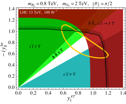
Direct searches at the LHC can play an important role in constraining LQ model(s) aiming to explain the and anomalies. In the following we show that the benchmark masses GeV and TeV are currently allowed by the high- and direct search experiments at the LHC and present exclusion limits for a projected LHC luminosity of 100 fb-1 of data.
High- di-tau tails
The dominant NP contributions to production, in view of the flavor structure of Eq. (4), come from the -channel exchange of and states in charm and bottom annihilation, respectively. Similar contributions from depend on the value of the mixing angle . As discussed in Sec. IV, the low-energy fit prefers . In this case an almost exact flavor alignment takes place between and the third quark generation, meaning that only the exchange of from initial collisions contributes to production. Following Ref. [57], we confront this scenario with data by recasting the most recent search by ATLAS [58] at 13 TeV and 36.1 fb-1 for a heavy resonance in the high-mass tails. Our results for the 95% C.L. limits in the – plane are given by the red exclusion region in Fig. 3 for the two benchmark masses, , and the LHC luminosity of 100 fb-1.
Leptoquark pair production
For the benchmark masses, bounds from pair-produced LQs can only be derived for . The dominant decay channels for each charged eigenstate are and with the corresponding branching fractions fixed by the squared ratio of Yukawa couplings . To set limits on , we use CMS results from the search [59] for final states and the multi-jet plus missing energy search [60] for final states, i.e., plus missing energy signature. The 95% C.L. exclusion limits are given by the light green and turquoise regions in Fig. 3 for a luminosity of 100 fb-1. As for the pair production of states, we employ the search by CMS [61] targeting final states. Results from this search are given by the dark green exclusion region in Fig. 3.
VI Conclusions
We propose a two scalar LQ extension of the SM that can accommodate all measured LFU ratios in -meson decays and related flavor observables, while being compatible with direct search constraints at the LHC. The extension has an origin that relates Yukawa couplings of the two LQs through a mixing angle and all Yukawas remain perturbative up to the unification scale. We provide prospects for future discoveries of the two light LQs at the LHC and spell out predictions for several yet-to-be-measured flavor observables. In particular, we predict and correlate with . We also predict a lower bound for which is just below the current experimental limit.
Acknowledgements.
S.F., D.A.F., and N.K. acknowledge support of the Slovenian Research Agency under the core funding grant P1-0035. This work has been supported in part by Croatian Science Foundation under the project 7118 and the European Union’s Horizon 2020 research and innovation programme under the Marie Sklodowska-Curie grant agreements N∘ 674896 and 690575.References
- [1] J. P. Lees et al. [BaBar Collaboration], Phys. Rev. D 88, no. 7, 072012 (2013) [arXiv:1303.0571 [hep-ex]].
- [2] S. Hirose et al. [Belle Collaboration], Phys. Rev. Lett. 118, no. 21, 211801 (2017) [arXiv:1612.00529 [hep-ex]].
- [3] R. Aaij et al. [LHCb Collaboration], Phys. Rev. Lett. 115, no. 11, 111803 (2015) Erratum: [Phys. Rev. Lett. 115, no. 15, 159901 (2015)] [arXiv:1506.08614 [hep-ex]].
- [4] J. A. Bailey et al. [MILC Collaboration], Phys. Rev. D 92, no. 3, 034506 (2015) [arXiv:1503.07237 [hep-lat]].
- [5] S. Fajfer, J. F. Kamenik and I. Nisandzic, Phys. Rev. D 85, 094025 (2012) [arXiv:1203.2654 [hep-ph]].
- [6] F. U. Bernlochner, Z. Ligeti, M. Papucci and D. J. Robinson, Phys. Rev. D 95, no. 11, 115008 (2017) Erratum: [Phys. Rev. D 97, no. 5, 059902 (2018)] [arXiv:1703.05330 [hep-ph]].
- [7] D. Bigi, P. Gambino and S. Schacht, Phys. Lett. B 769, 441 (2017) [arXiv:1703.06124 [hep-ph]].
- [8] R. Aaij et al. [LHCb Collaboration], Phys. Rev. Lett. 120, no. 12, 121801 (2018) [arXiv:1711.05623 [hep-ex]].
- [9] R. Aaij et al. [LHCb Collaboration], Phys. Rev. Lett. 113, 151601 (2014) [arXiv:1406.6482 [hep-ex]].
- [10] R. Aaij et al. [LHCb Collaboration], JHEP 1708, 055 (2017) [arXiv:1705.05802 [hep-ex]].
- [11] G. Hiller and F. Kruger, Phys. Rev. D 69, 074020 (2004) [hep-ph/0310219].
- [12] M. Bordone, G. Isidori and A. Pattori, Eur. Phys. J. C 76, no. 8, 440 (2016) [arXiv:1605.07633 [hep-ph]].
- [13] D. Buttazzo, A. Greljo, G. Isidori and D. Marzocca, JHEP 1711, 044 (2017) [arXiv:1706.07808 [hep-ph]].
- [14] B. Bhattacharya, A. Datta, D. London and S. Shivashankara, Phys. Lett. B 742, 370 (2015) [arXiv:1412.7164 [hep-ph]].
- [15] F. Feruglio, P. Paradisi and A. Pattori, Phys. Rev. Lett. 118, no. 1, 011801 (2017) [arXiv:1606.00524 [hep-ph]].
- [16] G. Hiller and M. Schmaltz, Phys. Rev. D 90, 054014 (2014) [arXiv:1408.1627 [hep-ph]].
- [17] N. Assad, B. Fornal and B. Grinstein, Phys. Lett. B 777 (2018) 324 [arXiv:1708.06350 [hep-ph]].
- [18] M. Bordone, C. Cornella, J. Fuentes-Martín and G. Isidori, arXiv:1805.09328 [hep-ph].
- [19] M. Bordone, C. Cornella, J. Fuentes-Martin and G. Isidori, Phys. Lett. B 779, 317 (2018) [arXiv:1712.01368 [hep-ph]].
- [20] A. Greljo and B. A. Stefanek, Phys. Lett. B 782, 131 (2018) [arXiv:1802.04274 [hep-ph]].
- [21] L. Di Luzio, A. Greljo and M. Nardecchia, Phys. Rev. D 96, no. 11, 115011 (2017) [arXiv:1708.08450 [hep-ph]].
- [22] M. Blanke and A. Crivellin, arXiv:1801.07256 [hep-ph].
- [23] L. Calibbi, A. Crivellin and T. Li, arXiv:1709.00692 [hep-ph].
- [24] A. Crivellin, D. Müller and T. Ota, JHEP 1709, 040 (2017) [arXiv:1703.09226 [hep-ph]].
- [25] D. Marzocca, arXiv:1803.10972 [hep-ph].
- [26] H. Georgi and S. L. Glashow, Phys. Rev. Lett. 32, 438 (1974).
- [27] T. Hubsch and S. Pallua, Phys. Lett. 138B, 279 (1984).
- [28] T. Hubsch, S. Meljanac and S. Pallua, Phys. Rev. D 31, 2958 (1985).
- [29] F. Staub, Comput. Phys. Commun. 185, 1773 (2014) [arXiv:1309.7223 [hep-ph]].
- [30] I. Dorsner, S. Fajfer and N. Kosnik, Phys. Rev. D 86, 015013 (2012) [arXiv:1204.0674 [hep-ph]].
- [31] I. Doršner, S. Fajfer and N. Košnik, Eur. Phys. J. C 77, no. 6, 417 (2017) [arXiv:1701.08322 [hep-ph]].
- [32] H. Na et al. [HPQCD Collaboration], Phys. Rev. D 92, no. 5, 054510 (2015) Erratum: [Phys. Rev. D 93, no. 11, 119906 (2016)] [arXiv:1505.03925 [hep-lat]].
- [33] J. P. Lees et al. [BaBar Collaboration], Phys. Rev. Lett. 109, 101802 (2012) [arXiv:1205.5442 [hep-ex]].
- [34] M. Huschle et al. [Belle Collaboration], Phys. Rev. D 92, no. 7, 072014 (2015) [arXiv:1507.03233 [hep-ex]].
- [35] R. Aaij et al. [LHCb Collaboration], Phys. Rev. D 97, no. 7, 072013 (2018) [arXiv:1711.02505 [hep-ex]].
- [36] Y. Amhis et al. [HFLAV Collaboration], Eur. Phys. J. C 77, no. 12, 895 (2017) [arXiv:1612.07233 [hep-ex]].
- [37] M. González-Alonso, J. Martin Camalich and K. Mimouni, Phys. Lett. B 772, 777 (2017) [arXiv:1706.00410 [hep-ph]].
- [38] I. Doršner, S. Fajfer, D. A. Faroughy and N. Košnik, JHEP 1710, 188 (2017) [arXiv:1706.07779 [hep-ph]].
- [39] R. Glattauer et al. [Belle Collaboration], Phys. Rev. D 93, no. 3, 032006 (2016) [arXiv:1510.03657 [hep-ex]].
- [40] A. Abdesselam et al. [Belle Collaboration], arXiv:1702.01521 [hep-ex].
- [41] D. Bečirević, N. Košnik, O. Sumensari and R. Zukanovich Funchal, JHEP 1611, 035 (2016) [arXiv:1608.07583 [hep-ph]].
- [42] V. Cirigliano and I. Rosell, Phys. Rev. Lett. 99, 231801 (2007) [arXiv:0707.3439 [hep-ph]].
- [43] D. Bečirević and O. Sumensari, JHEP 1708, 104 (2017) [arXiv:1704.05835 [hep-ph]].
- [44] G. D’Amico, M. Nardecchia, P. Panci, F. Sannino, A. Strumia, R. Torre and A. Urbano, JHEP 1709, 010 (2017) [arXiv:1704.05438 [hep-ph]].
- [45] B. Capdevila, A. Crivellin, S. Descotes-Genon, J. Matias and J. Virto, JHEP 1801, 093 (2018) [arXiv:1704.05340 [hep-ph]].
- [46] W. Altmannshofer, A. J. Buras, D. M. Straub and M. Wick, JHEP 0904, 022 (2009) [arXiv:0902.0160 [hep-ph]].
- [47] J. Grygier et al. [Belle Collaboration], Phys. Rev. D 96, no. 9, 091101 (2017) Addendum: [Phys. Rev. D 97, no. 9, 099902 (2018)] [arXiv:1702.03224 [hep-ex]].
- [48] C. Patrignani et al. [Particle Data Group], Chin. Phys. C 40, no. 10, 100001 (2016).
- [49] J. Beringer et al. [Particle Data Group], Phys. Rev. D 86, 010001 (2012).
- [50] S. Schael et al. [ALEPH and DELPHI and L3 and OPAL and SLD Collaborations and LEP Electroweak Working Group and SLD Electroweak Group and SLD Heavy Flavour Group], Phys. Rept. 427, 257 (2006) [hep-ex/0509008].
- [51] Y. Sakaki, M. Tanaka, A. Tayduganov and R. Watanabe, Phys. Rev. D 91 (2015) no.11, 114028 [arXiv:1412.3761 [hep-ph]].
- [52] D. Bečirević, B. Panes, O. Sumensari and R. Zukanovich Funchal, JHEP 1806 (2018) 032 [arXiv:1803.10112 [hep-ph]].
- [53] J. P. Lees et al. [BaBar Collaboration], Phys. Rev. D 86, 012004 (2012) [arXiv:1204.2852 [hep-ex]].
- [54] D. Bečirević, O. Sumensari and R. Zukanovich Funchal, Eur. Phys. J. C 76, no. 3, 134 (2016) [arXiv:1602.00881 [hep-ph]].
- [55] S. L. Glashow, D. Guadagnoli and K. Lane, Phys. Rev. Lett. 114 (2015) 091801 [arXiv:1411.0565 [hep-ph]].
- [56] D. Guadagnoli and K. Lane, Phys. Lett. B 751 (2015) 54 [arXiv:1507.01412 [hep-ph]].
- [57] D. A. Faroughy, A. Greljo and J. F. Kamenik, Phys. Lett. B 764, 126 (2017) [arXiv:1609.07138 [hep-ph]].
- [58] M. Aaboud et al. [ATLAS Collaboration], JHEP 1801, 055 (2018) [arXiv:1709.07242 [hep-ex]].
- [59] A. M. Sirunyan et al. [CMS Collaboration], JHEP 1707, 121 (2017) [arXiv:1703.03995 [hep-ex]].
- [60] CMS Collaboration [CMS Collaboration], CMS-PAS-SUS-16-036.
- [61] A. M. Sirunyan et al. [CMS Collaboration], arXiv:1803.02864 [hep-ex].