跳到论文正文
W Papers独立论文阅读器 arXiv:1806.05460 论文正文 计算阅读时间 · 0%
引用这篇论文根据当前论文元数据生成,正式投稿前建议核对。


License: arXiv.org perpetual non-exclusive license
arXiv:1806.05460v1 [math.PR] 14 Jun 2018

Semi-fractional diffusion equations

Peter Kern Address: Peter Kern, Mathematical Institute, Heinrich-Heine-University Düsseldorf, Universitätsstr. 1, D-40225 Düsseldorf, Germany Email address: kern@hhu.de , Svenja Lage Address: Svenja Lage, Mathematical Institute, Heinrich-Heine-University Düsseldorf, Universitätsstr. 1, D-40225 Düsseldorf, Germany Email address: Svenja.Lage@uni-duesseldorf.de and Mark M. Meerschaert Address: Mark M. Meerschaert, Department of Statistics and Probability, Michigan State University, East Lansing, MI 48824, USA Email address: mcubed@stt.msu.edu
Date: August 24, 2026
Abstract.

It is well known that certain fractional diffusion equations can be solved by the densities of stable Lévy motions. In this paper we use the classical semigroup approach for Lévy processes to define semi-fractional derivatives, which allows us to generalize this statement to semistable Lévy processes. A Fourier series approach for the periodic part of the corresponding Lévy exponents enables us to represent semi-fractional derivatives by a Grünwald-Letnikov type formula. We use this formula to calculate semi-fractional derivatives and solutions to semi-fractional diffusion equations numerically. In particular, by means of the Grünwald-Letnikov type formula we provide a numerical algorithm to compute semistable densities.

Key words and phrases: 
semistable Lévy process, log-characteristic function, log-periodic perturbation, semi-fractional derivative, Zolotarev fractional derivative, Grünwald-Letnikov type formula
2010 Mathematics Subject Classification
Primary 35R11, 60E10; Secondary 26A33, 60E07, 60G22, 60G51, 60H30, 82C31.

1. Introduction

Space-fractional diffusion equations are useful to model anomalous diffusions with a faster spreading rate than the classical Brownian motion model predicts [17]. In this case the behavior is super-diffusive and a spreading rate t1/αt^{1/\alpha} with time tt for some α∈(0,2)\alpha\in(0,2) may be modeled by a space-fractional partial differential equation

∂∂t​p​(x,t)=D1​∂α∂xα​p​(x,t)+D2​∂α∂(−x)α​p​(x,t)\frac{\partial}{\partial t}\,p(x,t)=D_{1}\,\frac{\partial^{\alpha}}{\partial x^{\alpha}}\,p(x,t)+D_{2}\,\frac{\partial^{\alpha}}{\partial(-x)^{\alpha}}\,p(x,t)

for constants D1,D2∈ℝD_{1},D_{2}\in{\mathbb{R}} with D1,D2≤0D_{1},D_{2}\leq 0 if α∈(0,1)\alpha\in(0,1) or D1,D2≥0D_{1},D_{2}\geq 0 if α∈(1,2)\alpha\in(1,2) and D1+D2≠0D_{1}+D_{2}\not=0 in both cases. Together with the initial condition p⁡(x,0)=δxp(x,0)=\delta_{x} (the Dirac delta distribution) the solution is well-known to consist of densities x↦p⁡(x,t)x\mapsto p(x,t) of a stable Lévy process (Xt)t≥0(X_{t})_{t\geq 0}; see [5, 15]. Here, ∂α∂xα\frac{\partial^{\alpha}}{\partial x^{\alpha}} and ∂α∂(−x)α\frac{\partial^{\alpha}}{\partial(-x)^{\alpha}} are the positive and negative fractional derivatives of order α∈(0,2)∖{1}\alpha\in(0,2)\setminus\{1\}. We refer to [11, 15, 18] for details on fractional derivatives, corresponding fractional partial differential equations and their connection to stochastic processes with heavy tails. Numerous applications of fractional diffusions are known from physics, biology, hydrology and other sciences; e.g., see [11, 15, 18] and the references cited therein.

Our goal is to generalize these fractional diffusion models so that the more general class of semistable Lévy process densities also appears as solutions of certain nonlocal diffusion equations which we will call semi-fractional. The difference between the stable and the semistable Lévy processes is that the power law behavior of the tails of the Lévy measure can additionally be disturbed by log-periodic functions as described below. Such log-periodic perturbations naturally appear in many physical applications [20] and also in finance [21]. We further aim to give numerical solutions to semi-fractional diffusion equations by means of a Grünwald-Letnikov type formula similar to [16] which also provides a method to calculate any semistable probability density numerically. To the best of our knowledge, the only available numerical method to calculate semistable probability densities is given in [4] by Laplace inversion techniques for the special case of one-sided semistable distributions.

For some fixed c>1c>1 and α∈(0,2]\alpha\in(0,2] a non-degenerate probability measure ν\nu is called (c1/α,c)(c^{1/\alpha},c)-semistable if ν\nu is infinitely divisible and there exists d∈ℝd\in\mathbb{R} such that

(1.1) ν∗c=(c1/α​ν)∗εd,\nu^{\ast c}=(c^{1/\alpha}\nu)\ast\varepsilon_{d},

where ν∗c\nu^{\ast c} is the cc-fold convolution power of ν\nu, well-defined by the Lévy-Khintchine representation [13, Theorem 3.1.11], (c1/α​ν)(c^{1/\alpha}\nu) is the image measure of ν\nu under the dilation x↦c1/α​xx\mapsto c^{1/\alpha}x and εd\varepsilon_{d} denotes the Dirac measure concentrated at d∈ℝd\in\mathbb{R}. If (1.1) holds for every c>1c>1 and some d=d⁡(c)∈ℝd=d(c)\in\mathbb{R} then ν\nu is α\alpha-stable and thus semistability generalizes stability with a discrete scaling property. If α=2\alpha=2, then ν\nu is a normal law and thus stable. We will exclude this case in our considerations and thus for α∈(0,2)\alpha\in(0,2) the Fourier transform ν^​(x)=∫ℝei​x​y​𝑑ν​(y)=exp⁡(ψ⁡(x))\widehat{\nu}(x)=\int_{{\mathbb{R}}}e^{ixy}\,d\nu(y)=\exp(\psi(x)) is given by the log-characteristic function

(1.2) ψ⁡(x)=i​a​x+∫ℝ∖{0}(ei​x​y−1−i​x​y1+y2)​𝑑ϕ​(y)\psi(x)=iax+\int\limits_{\mathbb{R}\setminus\{0\}}\left(e^{ixy}-1-\frac{ixy}{1+y^{2}}\right)d\phi(y)

for some unique a∈ℝa\in{\mathbb{R}} and a Lévy measure ϕ\phi determined by

ϕ⁡(r,∞)=r−α​θ1​(log⁡r) and ϕ⁡(−∞,−r)=r−α​θ2​(log⁡r)\phi(r,\infty)=r^{-\alpha}\theta_{1}(\log r)\quad\text{ and }\quad\phi(-\infty,-r)=r^{-\alpha}\theta_{2}(\log r)

for every r>0r>0, where θ1,θ2:ℝ→[0,∞)\theta_{1},\theta_{2}:\mathbb{R}\to[0,\infty) are log⁡(c1/α)\log(c^{1/\alpha})-periodic functions, such that θ:=θ1+θ2\theta:=\theta_{1}+\theta_{2} is strictly positive. Due to the fact that ϕ\phi is a measure, we know that r↦r−α​θ​(log⁡r)r\mapsto r^{-\alpha}\theta(\log r) is non-increasing, equivalently θ\theta fulfills the growth restriction

(1.3) θ⁡(y+δ)≤eα​δ​θ​(y) for every ​y∈ℝ​ and ​δ≥0\theta(y+\delta)\leq e^{\alpha\delta}\theta(y)\quad\text{ for every }y\in{\mathbb{R}}\text{ and }\delta\geq 0

and (1.3) carries over to θ1\theta_{1} and θ2\theta_{2} instead of θ\theta. For more details on semistable distributions we refer the reader to the monographs [13] and [19].

The following result is from Theorem 3.17 of [15]. Let (Xt)t≥0(X_{t})_{t\geq 0} be a Lévy process with Fourier transform 𝔼⁡[exp⁡(i​x​Xt)]=exp⁡(t​ψ​(x)){\mathbb{E}}[\exp(ixX_{t})]=\exp(t\,\psi(x)), then the family of linear operators (Tt)t≥0(T_{t})_{t\geq 0} given by

Tt​f​(x):=𝔼⁡[f⁡(x−Xt)] for all ​t≥0​ and ​x∈ℝT_{t}f(x):={\mathbb{E}}[f(x-X_{t})]\quad\text{ for all }t\geq 0\text{ and }x\in{\mathbb{R}}

determines a C0C_{0}-semigroup for functions ff in C0​(ℝ)C_{0}(\mathbb{R}) with generator

(1.4) L​f​(x)=−a​f′​(x)+∫ℝ∖{0}(f⁡(x−y)−f⁡(x)+y​f′​(x)1+y2)​𝑑ϕ​(y),Lf(x)=-af^{\prime}(x)+\int\limits_{\mathbb{R}\setminus\{0\}}\left(f(x-y)-f(x)+\frac{yf^{\prime}(x)}{1+y^{2}}\right)d\phi(y),

where at least functions ff with f,f′,f′′∈C0​(ℝ)∩L1​(ℝ)f,f^{\prime},f^{\prime\prime}\in C_{0}(\mathbb{R})\cap L^{1}(\mathbb{R}) belong to the domain of the generator, and we have

(1.5) L​f^​(x)=ψ⁡(x)​f^​(x) for all ​x∈ℝ,\widehat{Lf}(x)=\psi(x)\widehat{f}(x)\quad\text{ for all }x\in\mathbb{R},

where ψ\psi is the log-characteristic function in (1.2) and the Fourier transform of a function f∈L1​(ℝ)f\in L^{1}({\mathbb{R}}) is given by f^​(x)=∫ℝei​x​y​f​(y)​𝑑y\widehat{f}(x)=\int_{{\mathbb{R}}}e^{ixy}f(y)\,dy.

This is our starting point to introduce semi-fractional derivatives in Section 2 in terms of the generators of semistable semigroups. Using a Fourier series approach for the periodic functions θ1,θ2\theta_{1},\theta_{2} we will establish a series representation of the log-characteristic function in Section 3 which sheds some light on semi-fractional derivatives. The Fourier series approach also enables us to give a useful numerical approximation formula to semi-fractional derivatives by a Grünwald-Letnikov type formula in Section 4. Finally, in Section 5 we consider semi-fractional diffusion equations for which the densities of semi-stable Lévy processes are a valid solution. These densities are then approximated numerically by means of our Grünwald-Letnikov type formula.

2. Semi-fractional derivatives and diffusion equations

We introduce the following notation for periodic functions suitably appearing in the log-characteristic function of a semistable law.

Definition 2.1.

Given c>1c>1 and α∈(0,2)\alpha\in(0,2) we call a function θ:ℝ→(0,∞)\theta:{\mathbb{R}}\to(0,\infty) admissable if θ\theta is log⁡(c1/α)\log(c^{1/\alpha})-periodic and fulfills the growth restriction (1.3). An admissable function θ\theta as above is called smooth if θ\theta is continuous on ℝ{\mathbb{R}} and piecewise continuously differentiable.

We will now define semi-fractional derivatives as a direct generalization of classical fractional derivatives by their generator form. For details on the connection of ordinary fractional derivatives and stable distributions we refer to [15]. Note that the generators of semistable Lévy processes have been used in [14] to approximate fractional derivatives as c↓1c\downarrow 1. As in the special case of classical fractional derivatives, we will distinguish between the cases α∈(0,1)\alpha\in(0,1) and α∈(1,2)\alpha\in(1,2) and between Lévy measures concentrated on the positive or negative half-line. We will need the following auxiliary result for α∈(1,2)\alpha\in(1,2).

Lemma 2.2.

Given c>1c>1, α∈(1,2)\alpha\in(1,2) and a corresponding admissable function θ\theta we have

(2.1) ∫y∞x−α​θ​(log⁡x)​𝑑x=y1−α​γ​(log⁡y) for all ​y>0,\int_{y}^{\infty}x^{-\alpha}\theta(\log x)\,dx=y^{1-\alpha}\gamma(\log y)\quad\text{ for all }y>0,

where γ\gamma is the continuous admissable function given by

(2.2) γ⁡(x)=e(α−1)​x​∫ex∞y−α​θ​(log⁡y)​𝑑y for all ​x∈ℝ.\gamma(x)=e^{(\alpha-1)x}\int_{e^{x}}^{\infty}y^{-\alpha}\theta(\log y)\,dy\quad\text{ for all }x\in{\mathbb{R}}.
Proof.

Clearly, from (2.2) it follows that γ\gamma is continuous and γ⁡(x)∈(0,∞)\gamma(x)\in(0,\infty) for all x∈ℝx\in{\mathbb{R}}. Further, γ\gamma fulfills the growth restriction (1.3), since the left-hand side in (2.1) is strictly decreasing, and by a change of variables y=z​c1/αy=z\,c^{1/\alpha} we get

γ⁡(x+log⁡c1/α)\displaystyle\gamma(x+\log c^{1/\alpha}) =e(α−1)​x​c(α−1)/α​∫ex​c1/α∞y−α​θ​(log⁡y)​𝑑y\displaystyle=e^{(\alpha-1)x}c^{(\alpha-1)/\alpha}\int_{e^{x}c^{1/\alpha}}^{\infty}y^{-\alpha}\theta(\log y)\,dy
=e(α−1)​x​c​∫ex∞(z​c1/α)−α​θ​(log⁡z+log⁡c1/α)​𝑑z=γ⁡(x)\displaystyle=e^{(\alpha-1)x}c\int_{e^{x}}^{\infty}(z\,c^{1/\alpha})^{-\alpha}\theta(\log z+\log c^{1/\alpha})\,dz=\gamma(x)

for all x∈ℝx\in{\mathbb{R}}, showing that γ\gamma is an admissable function. ∎

2.1. Semi-fractional derivatives

We will first consider α∈(0,1)\alpha\in(0,1). Given c>1c>1 and α∈(0,1)\alpha\in(0,1) let ϕ1\phi_{1} be the Lévy measure given by

(2.3) ϕ1​(r,∞)=r−α​θ​(log⁡r) and ϕ1​(−∞,−r)=0\phi_{1}(r,\infty)=r^{-\alpha}\theta(\log r)\quad\text{ and }\quad\phi_{1}(-\infty,-r)=0

for all r>0r>0 and some fixed admissable function θ\theta. Let

a1:=∫0+∞y1+y2​d​ϕ1​(y),a_{1}:=\int\limits_{0+}^{\infty}\frac{y}{1+y^{2}}\,d\phi_{1}(y),

which is a positive and finite constant, and write L1L_{1} for the corresponding generator in (1.4) with a=a1a=a_{1} and ϕ=ϕ1\phi=\phi_{1}. Then the generator takes a simpler form:

Definition 2.3.

With the above assumptions, for a function ff belonging to the domain of L1L_{1} we define the positive (or left-sided) semi-fractional derivative of order α∈(0,1)\alpha\in(0,1) with respect to cc, θ\theta by its generator form

∂α∂c,θxα​f​(x):=−L1​f​(x)=∫0+∞(f⁡(x)−f⁡(x−y))​d​ϕ1​(y).\displaystyle\frac{\partial^{\alpha}}{\partial_{c,\theta}x^{\alpha}}\,f(x):=-L_{1}f(x)=\int_{0+}^{\infty}(f(x)-f(x-y))\,d\phi_{1}(y).

By reflection of the Lévy measure ϕ1\phi_{1} we get a new Lévy measure ϕ2\phi_{2} on the negative half-line with

ϕ2​(r,∞)=0 and ϕ2​(−∞,−r)=r−α​θ​(log⁡r)\phi_{2}(r,\infty)=0\quad\text{ and }\quad\phi_{2}(-\infty,-r)=r^{-\alpha}\theta(\log r)

for all r>0r>0. Write L2L_{2} for the corresponding generator in (1.4) with ϕ=ϕ2\phi=\phi_{2} and

a=a2:=∫−∞0−y1+y2dϕ2(y)=−∫0+∞y1+y2dϕ1(y)=−a1.a=a_{2}:=\int\limits_{-\infty}^{0-}\frac{y}{1+y^{2}}\,d\phi_{2}(y)=-\int_{0+}^{\infty}\frac{y}{1+y^{2}}\,d\phi_{1}(y)=-a_{1}.

By a change of variables y↦−yy\mapsto-y in (1.4), we may express L2L_{2} in terms of the Lévy measure ϕ1\phi_{1} from (2.3). Then the generator takes a simpler form, similar to the nonlocal operator in Definition 2.3, but involving the values of f⁡(y)f(y) for y>xy>x:

Definition 2.4.

With the above assumptions, for a function ff belonging to the domain of L2L_{2} we define the negative (or right-sided) semi-fractional derivative of order α∈(0,1)\alpha\in(0,1) with respect to cc, θ\theta by

∂α∂c,θ(−x)α​f​(x):=−L2​f​(x)=∫0+∞(f⁡(x)−f⁡(x+y))​d​ϕ1​(y).\displaystyle\frac{\partial^{\alpha}}{\partial_{c,\theta}(-x)^{\alpha}}\,f(x):=-L_{2}f(x)=\int_{0+}^{\infty}(f(x)-f(x+y))\,d\phi_{1}(y).

For functions ff with f,f′,f′′∈C0​(ℝ)∩L1​(ℝ)f,f^{\prime},f^{\prime\prime}\in C_{0}(\mathbb{R})\cap L^{1}(\mathbb{R}) we know that the fractional derivative of order α∈(0,1)\alpha\in(0,1) exists and integration by parts in combination with (2.3) yields the equivalent Caputo form

∂α∂c,θxα​f​(x)\displaystyle\frac{\partial^{\alpha}}{\partial_{c,\theta}x^{\alpha}}\,f(x) =[(f⁡(x−y)−f⁡(x))​y−α​θ​(log⁡y)]y=0+∞+∫0+∞f′​(x−y)​y−α​θ​(log⁡y)​𝑑y\displaystyle=\left[(f(x-y)-f(x))y^{-\alpha}\theta(\log y)\right]_{y=0+}^{\infty}+\int_{0+}^{\infty}f^{\prime}(x-y)y^{-\alpha}\theta(\log y)\,dy
=∫0+∞f′​(x−y)​y−α​θ​(log⁡y)​𝑑y,\displaystyle=\int_{0+}^{\infty}f^{\prime}(x-y)y^{-\alpha}\theta(\log y)\,dy,

where the first term vanishes since θ\theta is bounded, f,f′∈C0​(ℝ)f,f^{\prime}\in C_{0}(\mathbb{R}) and thus for some constant C>0C>0 we have

limy↓0|(f⁡(x−y)−f⁡(x))​y−α​θ​(log⁡y)|\displaystyle\lim\limits_{y\downarrow 0}|(f(x-y)-f(x)){y^{-\alpha}}\theta(\log y)| ≤C​limy↓0|f⁡(x−y)−f⁡(x)|​y−α\displaystyle\leq C\lim\limits_{y\downarrow 0}|f(x-y)-f(x)|y^{-\alpha}
=C​|f′​(x)|​limy↓0y1−α=0.\displaystyle=C|f^{\prime}(x)|\lim\limits_{y\downarrow 0}y^{1-\alpha}=0.

Analogously, the Caputo form of the negative semi-fractional derivative of order α∈(0,1)\alpha\in(0,1) is given by

∂α∂c,θ(−x)α​f​(x)\displaystyle\frac{\partial^{\alpha}}{\partial_{c,\theta}(-x)^{\alpha}}\,f(x) =−∫0+∞f′(x+y)y−αθ(logy)dy.\displaystyle=-\int_{0+}^{\infty}f^{\prime}(x+y)y^{-\alpha}\theta(\log y)\,dy.

Note that for constant θ≡1/Γ⁡(1−α)>0\theta\equiv 1/\Gamma(1-\alpha)>0 we get back the usual (positive and negative) Caputo fractional derivatives of order α∈(0,1)\alpha\in(0,1).

Now we will consider α∈(1,2)\alpha\in(1,2). Given c>1c>1 and α∈(1,2)\alpha\in(1,2) let ϕ1\phi_{1} be as above and define

a3:=∫0+∞(y1+y2−y)​d​ϕ1​(y),a_{3}:=\int\limits_{0+}^{\infty}\left(\frac{y}{1+y^{2}}-y\right)\,d\phi_{1}(y),

which is a real constant due to our assumptions. Write L3L_{3} for the corresponding generator in (1.4) with a=a3a=a_{3} and ϕ=ϕ1\phi=\phi_{1}. Then the generator equation (1.4) takes a simpler form:

Definition 2.5.

With the above assumptions, for a function ff belonging to the domain of L3L_{3} we define the semi-fractional derivative of order α∈(1,2)\alpha\in(1,2) with respect to cc, θ\theta by its generator form

∂α∂c,θxα​f​(x):=L3​f​(x)=∫0+∞(f⁡(x−y)−f⁡(x)+y​f′​(x))​d​ϕ1​(y).\displaystyle\frac{\partial^{\alpha}}{\partial_{c,\theta}x^{\alpha}}\,f(x):=L_{3}f(x)=\int_{0+}^{\infty}(f(x-y)-f(x)+y\,f^{\prime}(x))\,d\phi_{1}(y).

Again, by reflection of the Lévy measure ϕ1\phi_{1} we get the Lévy measure ϕ2\phi_{2} on the negative half-line and we write L4L_{4} for the corresponding generator in (1.4) with

a=a4:=∫−∞0−(y1+y2−y)dϕ2(y)=−∫0+∞(y1+y2−y)dϕ1(y)=−a3.a=a_{4}:=\int\limits_{-\infty}^{0-}\left(\frac{y}{1+y^{2}}-y\right)\,d\phi_{2}(y)=-\int\limits_{0+}^{\infty}\left(\frac{y}{1+y^{2}}-y\right)\,d\phi_{1}(y)=-a_{3}.

Again, by a change of variables y↦−yy\mapsto-y in (1.4), we may express L4L_{4} in terms of the Lévy measure ϕ1\phi_{1} from (2.3). With this Lévy measure and the above shift, we obtain the following generator:

Definition 2.6.

With the above assumptions, for a function ff belonging to the domain of L4L_{4} we define the negative semi-fractional derivative of order α∈(1,2)\alpha\in(1,2) with respect to cc, θ\theta by

∂α∂c,θ(−x)α​f​(x):=L4​f​(x)=∫0+∞(f⁡(x+y)−f⁡(x)−y​f′​(x))​d​ϕ1​(y).\displaystyle\frac{\partial^{\alpha}}{\partial_{c,\theta}(-x)^{\alpha}}\,f(x):=L_{4}f(x)=\int_{0+}^{\infty}(f(x+y)-f(x)-y\,f^{\prime}(x))\,d\phi_{1}(y).

As before, for functions ff with f,f′,f′′∈C0​(ℝ)∩L1​(ℝ)f,f^{\prime},f^{\prime\prime}\in C_{0}(\mathbb{R})\cap L^{1}(\mathbb{R}) we know that the (negative) fractional derivative of order α∈(1,2)\alpha\in(1,2) exists. Integrate by parts twice to obtain the equivalent Caputo forms

(2.4) ∂α∂c,θxα​f​(x)=∫0+∞(f′​(x)−f′​(x−y))​y−α​θ​(log⁡y)​𝑑y=∫0+∞f′′​(x−y)​y1−α​γ​(log⁡y)​dy,\begin{split}\frac{\partial^{\alpha}}{\partial_{c,\theta}x^{\alpha}}\,f(x)&=\int_{0+}^{\infty}\left(f^{\prime}(x)-f^{\prime}(x-y)\right)y^{-\alpha}\theta(\log y)\,dy\\ &=\int_{0+}^{\infty}f^{\prime\prime}(x-y)\,y^{1-\alpha}\gamma(\log y)\,dy,\end{split}

where γ\gamma is the function from Lemma 2.2, using that f′,f′′∈C0​(ℝ)f^{\prime},f^{\prime\prime}\in C_{0}(\mathbb{R}) and the fact that γ\gamma is bounded, we obtain for some constant C>0C>0

limy↓0|(f⁡(x−y)−f⁡(x))​y1−α​γ​(log⁡y)|\displaystyle\lim\limits_{y\downarrow 0}\left|(f(x-y)-f(x))y^{1-\alpha}\gamma(\log y)\right| ≤C​limy↓0|(f⁡(x−y)−f⁡(x))|​y1−α\displaystyle\leq C\lim\limits_{y\downarrow 0}\left|(f(x-y)-f(x))\right|y^{1-\alpha}
≤C​|f′′​(x)|​limy↓0y2−α=0.\displaystyle\leq C|f^{\prime\prime}(x)|\lim_{y\downarrow 0}y^{2-\alpha}=0.

Analogously we get

∂α∂c,θ(−x)α​f​(x)\displaystyle\frac{\partial^{\alpha}}{\partial_{c,\theta}(-x)^{\alpha}}\,f(x) =∫0+∞(f′​(x+y)−f′​(x))​y−α​θ​(log⁡y)​𝑑y\displaystyle=\int_{0+}^{\infty}\left(f^{\prime}(x+y)-f^{\prime}(x)\right)y^{-\alpha}\theta(\log y)\,dy
=∫0+∞f′′​(x+y)​y1−α​γ​(log⁡y)​𝑑y.\displaystyle=\int_{0+}^{\infty}f^{\prime\prime}(x+y)\,y^{1-\alpha}\gamma(\log y)\,dy.

Note that for constant θ≡(α−1)/Γ(2−α)=−1/Γ(1−α)>0\theta\equiv(\alpha-1)/\Gamma(2-\alpha)=-1/\Gamma(1-\alpha)>0, i.e. γ≡1/Γ⁡(2−α)\gamma\equiv 1/\Gamma(2-\alpha), we get back the usual positive and negative) Caputo fractional derivatives of order α∈(1,2)\alpha\in(1,2).

2.2. Zolotarev derivative and ballistic scaling

In our previous considerations we have excluded the case α=1\alpha=1 and we now briefly illustrate by an example the technical difficulties that may arise for α=1\alpha=1. A prominent example of a semistable distribution is the limit distribution of cumulated gains in a sequence of St. Petersburg games, where c=2c=2 and α=1\alpha=1. The Lévy measure of the semistable limit distribution was first established in [12] and is the discrete measure ϕ1\phi_{1} given by

ϕ1​(2k)=2−k for all ​k∈ℤ.\phi_{1}(2^{k})=2^{-k}\quad\text{ for all }k\in{\mathbb{Z}}.

One can easily show that for r>0r>0 we have

ϕ1​(r,∞)=r−α​θ​(log⁡r) and ϕ1​(−∞,−r)=0,\phi_{1}(r,\infty)=r^{-\alpha}\theta(\log r)\quad\text{ and }\quad\phi_{1}(-\infty,-r)=0,

where θ\theta is the admissable function

θ⁡(x)=exp⁡(x−⌊xlog⁡2⌋​log⁡2) for all ​x∈ℝ.\theta(x)=\exp\left(x-\left\lfloor\frac{x}{\log 2}\right\rfloor\log 2\right)\quad\text{ for all }x\in{\mathbb{R}}.

We further obtain

a1\displaystyle a_{1} =∫0+∞y1+y2​d​ϕ1​(y)=∑k=−∞∞11+4k=∞\displaystyle=\int\limits_{0+}^{\infty}\frac{y}{1+y^{2}}\,d\phi_{1}(y)=\sum_{k=-\infty}^{\infty}\frac{1}{1+4^{k}}=\infty
and
a3\displaystyle a_{3} =∫0+∞(y1+y2−y)dϕ1(y)=−∫0+∞y31+y2dϕ1(y)=−∑k=−∞∞11+4−k=−∞.\displaystyle=\int\limits_{0+}^{\infty}\left(\frac{y}{1+y^{2}}-y\right)\,d\phi_{1}(y)=-\int\limits_{0+}^{\infty}\frac{y^{3}}{1+y^{2}}\,d\phi_{1}(y)=-\sum_{k=-\infty}^{\infty}\frac{1}{1+4^{-k}}=-\infty.

Hence, both Definitions 2.3 and 2.5 fail to give a suitable semi-fractional derivative in this special case with α=1\alpha=1. To overcome this problem, recently in [10] the Zolotarev fractional derivative was introduced. In the ballistic case α=1\alpha=1 a direct generalization of the Zolotarev fractional derivative in [10] to our semistable situation is the following. As in Section 3.2.3 of [9] we define

a=a5:=∫0+∞(y1+y2−sin⁡y)​d​ϕ1​(y)a=a_{5}:=\int_{0+}^{\infty}\left(\frac{y}{1+y^{2}}-\sin y\right)\,d\phi_{1}(y)

in the Lévy-Khintchine representation (1.2) of the log-characteristic function ψ\psi with Lévy measure ϕ1\phi_{1} as above and write L𝒵+L_{\mathcal{Z}}^{+} for the corresponding generator in (1.4):

Definition 2.7.

With the above assumptions, for a function ff belonging to the domain of L𝒵+L_{\mathcal{Z}}^{+} we define the positive Zolotarev semi-fractional derivative of order α=1\alpha=1 with respect to cc, θ\theta by its generator form

∂𝒵∂c,θx​f​(x):=L𝒵+​f​(x)=∫0+∞(f⁡(x−y)−f⁡(x)+f′​(x)​sin⁡y)​d​ϕ1​(y).\displaystyle\frac{\partial_{\mathcal{Z}}}{\partial_{c,\theta}x}\,f(x):=L_{\mathcal{Z}}^{+}f(x)=\int_{0+}^{\infty}(f(x-y)-f(x)+f^{\prime}(x)\sin y)\,d\phi_{1}(y).

Note that for functions ff with f,f′,f′′∈C0​(ℝ)∩L1​(ℝ)f,f^{\prime},f^{\prime\prime}\in C_{0}(\mathbb{R})\cap L^{1}(\mathbb{R}) by the mean value theorem we observe for some ξ∈[x−y,x]\xi\in[x-y,x] and η∈[ξ,x]\eta\in[\xi,x]

f⁡(x−y)−f⁡(x)+f′​(x)​sin⁡y\displaystyle f(x-y)-f(x)+f^{\prime}(x)\sin y =−y​f′​(ξ)+f′​(x)​sin⁡y\displaystyle=-y\,f^{\prime}(\xi)+f^{\prime}(x)\sin y
=f′​(x)​(sin⁡y−y)+y⁡(f′​(x)−f′​(ξ))\displaystyle=f^{\prime}(x)(\sin y-y)+y\,(f^{\prime}(x)-f^{\prime}(\xi))
=f′​(x)​(sin⁡y−y)+y⁡(x−ξ)​f′′​(η)\displaystyle=f^{\prime}(x)(\sin y-y)+y\,(x-\xi)f^{\prime\prime}(\eta)

showing that as y↓0y\downarrow 0

|f⁡(x−y)−f⁡(x)+f′​(x)​sin⁡y|≤‖f′‖∞​|sin⁡y−y|+y2​‖f′′‖∞=O⁡(y2).\left|f(x-y)-f(x)+f^{\prime}(x)\sin y\right|\leq\|f^{\prime}\|_{\infty}|\sin y-y|+y^{2}\|f^{\prime\prime}\|_{\infty}=O(y^{2}).

Hence the Zolotarev semi-fractional derivative of order α=1\alpha=1 exists for such functions and integration by parts yields the Caputo form

∂𝒵∂c,θx​f​(x)=∫0+∞(f′​(x)​cos⁡y−f′​(x−y))​y−1​θ​(log⁡y)​𝑑y.\frac{\partial_{\mathcal{Z}}}{\partial_{c,\theta}x}\,f(x)=\int_{0+}^{\infty}\left(f^{\prime}(x)\cos y-f^{\prime}(x-y)\right)y^{-1}\theta(\log y)\,dy.

Note that for constant θ≡2/π\theta\equiv 2/\pi we get back the Zolotarev fractional derivative of order α=1\alpha=1 in [10].

Again, by reflection of the Lévy measure ϕ1\phi_{1} we get the Lévy measure ϕ2\phi_{2} on the negative half-line and we write L𝒵−L_{\mathcal{Z}}^{-} for the corresponding generator in (1.4) with

a:=∫−∞0−(y1+y2−siny)dϕ2(y)=−∫0+∞(y1+y2−siny)dϕ1(y)=−a5,a:=\int_{-\infty}^{0-}\left(\frac{y}{1+y^{2}}-\sin y\right)\,d\phi_{2}(y)=-\int_{0+}^{\infty}\left(\frac{y}{1+y^{2}}-\sin y\right)\,d\phi_{1}(y)=-a_{5},

then, by a change of variables y↦−yy\mapsto-y in (1.4), this generator takes the simpler form:

Definition 2.8.

With the above assumptions, for a function ff belonging to the domain of L𝒵−L_{\mathcal{Z}}^{-} we define the negative Zolotarev semi-fractional derivative of order α=1\alpha=1 with respect to cc, θ\theta by its generator form

∂𝒵∂c,θ(−x)​f​(x):=L𝒵−​f​(x)=∫0+∞(f⁡(x+y)−f⁡(x)−f′​(x)​sin⁡y)​d​ϕ1​(y).\displaystyle\frac{\partial_{\mathcal{Z}}}{\partial_{c,\theta}(-x)}\,f(x):=L_{\mathcal{Z}}^{-}f(x)=\int_{0+}^{\infty}(f(x+y)-f(x)-f^{\prime}(x)\sin y)\,d\phi_{1}(y).

As before, for functions ff with f,f′,f′′∈C0​(ℝ)∩L1​(ℝ)f,f^{\prime},f^{\prime\prime}\in C_{0}(\mathbb{R})\cap L^{1}(\mathbb{R}) the negative Zolotarev semi-fractional derivative of order α=1\alpha=1 exists and integration by parts yields the Caputo form

∂𝒵∂c,θ(−x)​f​(x)=∫0+∞(f′​(x+y)−f′​(x)​cos⁡y)​y−1​θ​(log⁡y)​𝑑y.\frac{\partial_{\mathcal{Z}}}{\partial_{c,\theta}(-x)}\,f(x)=\int_{0+}^{\infty}\left(f^{\prime}(x+y)-f^{\prime}(x)\cos y\right)y^{-1}\theta(\log y)\,dy.

3. semistable log-characteristic functions

An alternative, equivalent definition of the semi-fractional derivative using the Lévy-Khintchine representation (1.2) together with (1.5) is the following. Given c>1c>1, α∈(0,2)∖{1}\alpha\in(0,2)\setminus\{1\} and a corresponding admissable function θ\theta, with our choice of the shift a1a_{1} for α∈(0,1)\alpha\in(0,1) and a3a_{3} for α∈(1,2)\alpha\in(1,2), we may define ∂αf/∂c,θxα\partial^{\alpha}f/\partial_{c,\theta}x^{\alpha} as the function with Fourier transform

(3.1) ∂αf∂c,θxα^​(x)={−L1​f^(x)=−∫0+∞(ei​x​y−1)dϕ1(y)f^(x) if ​α∈(0,1),L3​f^​(x)=∫0+∞(ei​x​y−1−i​x​y)​d​ϕ1​(y)​f^​(x) if ​α∈(1,2),\widehat{\frac{\partial^{\alpha}f}{\partial_{c,\theta}x^{\alpha}}}(x)=\begin{cases}\displaystyle-\widehat{L_{1}f}(x)=-\int_{0+}^{\infty}(e^{ixy}-1)\,d\phi_{1}(y)\,\widehat{f}(x)&\text{ if }\alpha\in(0,1),\\[8.61108pt] \displaystyle\widehat{L_{3}f}(x)=\int_{0+}^{\infty}(e^{ixy}-1-ixy)\,d\phi_{1}(y)\,\widehat{f}(x)&\text{ if }\alpha\in(1,2),\end{cases}

for suitable functions ff. Analogously, with the shift a2a_{2} for α∈(0,1)\alpha\in(0,1) and a4a_{4} for α∈(1,2)\alpha\in(1,2), we can define ∂αf/∂c,θ(−x)α\partial^{\alpha}f/\partial_{c,\theta}(-x)^{\alpha} as the function with Fourier transform

(3.2) ∂αf∂c,θ(−x)α^​(x)={−L2​f^(x)=−∫0+∞(e−i​x​y−1)dϕ1(y)f^(x) if ​α∈(0,1),L4​f^​(x)=∫0+∞(e−i​x​y−1+i​x​y)​d​ϕ1​(y)​f^​(x) if ​α∈(1,2).\widehat{\frac{\partial^{\alpha}f}{\partial_{c,\theta}(-x)^{\alpha}}}(x)=\begin{cases}\displaystyle-\widehat{L_{2}f}(x)=-\int_{0+}^{\infty}(e^{-ixy}-1)\,d\phi_{1}(y)\,\widehat{f}(x)&\text{ if }\alpha\in(0,1),\\[8.61108pt] \displaystyle\widehat{L_{4}f}(x)=\int_{0+}^{\infty}(e^{-ixy}-1+ixy)\,d\phi_{1}(y)\,\widehat{f}(x)&\text{ if }\alpha\in(1,2).\end{cases}

for suitable functions ff, as well as the positive Zolotarev semi-fractional derivative for α=1\alpha=1 (using the shift a5a_{5}) as the function with Fourier transform

(3.3) ∂𝒵f∂c,θxα^​(x)=L𝒵+​f^​(x)=∫0+∞(ei​x​y−1−i​x​sin⁡(y))​d​ϕ1​(y)​f^​(x),\displaystyle\widehat{\frac{\partial_{\mathcal{Z}}f}{\partial_{c,\theta}x^{\alpha}}}(x)=\widehat{L_{\mathcal{Z}}^{+}f}(x)=\int_{0+}^{\infty}(e^{ixy}-1-ix\sin(y))\,d\phi_{1}(y)\,\widehat{f}(x),

respectively

(3.4) ∂𝒵f∂c,θ(−x)α^​(x)=L𝒵−​f^​(x)=∫0+∞(e−i​x​y−1+i​x​sin⁡(y))​d​ϕ1​(y)​f^​(x)\displaystyle\widehat{\frac{\partial_{\mathcal{Z}}f}{\partial_{c,\theta}(-x)^{\alpha}}}(x)=\widehat{L_{\mathcal{Z}}^{-}f}(x)=\int_{0+}^{\infty}(e^{-ixy}-1+ix\sin(y))\,d\phi_{1}(y)\,\widehat{f}(x)

for the negative Zolotarev semi-fractional derivative.

Our aim is to reduce (3.1) – (3.4) to simpler forms. Since the right-hand sides in (3.1) – (3.4) coincide with ∓ψ⁡(x)​f^​(x)\mp\psi(x)\,\widehat{f}(x) for the log-characteristic functions ψ\psi without drift part, corresponding to the generators L1L_{1} to L4L_{4} in Definitions 2.3–2.6 and L𝒵±L_{\mathcal{Z}}^{\pm} in Definitions 2.7 and 2.8, we will now derive a series representation of ψ\psi depending on the Fourier coefficients of the periodic function θ\theta, provided θ\theta is a smooth admissable function. This will directly provide us with a series representation of the Fourier transform of semi-fractional derivatives and will also enable us to give a formula of Grünwald-Letnikov type for the semi-fractional derivatives in Section 4. Given c>1c>1 and α∈(0,2)\alpha\in(0,2), let θ\theta be a smooth admissable function as in Definition 2.1. In this case for all x∈ℝx\in{\mathbb{R}} we have the Fourier series representation

(3.5) θ⁡(x)=∑k=−∞∞ck​ei​k​c~​x with c~:=2​π​αlog⁡c\theta(x)=\sum_{k=-\infty}^{\infty}c_{k}e^{ik\tilde{c}x}\quad\text{ with }\quad\tilde{c}:=\frac{2\pi\alpha}{\log c}

and the Fourier coefficients (ck)k∈ℤ⊆ℂ(c_{k})_{k\in\mathbb{Z}}\subseteq\mathbb{C} fulfill

c−k¯=ck and |ck|≤Ck2 for all ​k∈ℤ∖{0}​ and some ​C>0;\overline{c_{-k}}=c_{k}\quad\text{ and }\quad|c_{k}|\leq\frac{C}{k^{2}}\quad\text{ for all }k\in{\mathbb{Z}}\setminus\{0\}\text{ and some }C>0;

e.g., see [7] for details.

3.1. Log-characteristic function for α≠1\alpha\not=1

Theorem 3.1.

Given c>1c>1, α∈(0,2)∖{1}\alpha\in(0,2)\setminus\{1\} and a corresponding smooth admissable function θ\theta with Fourier series representation (3.5), let ψ\psi denote the log-characteristic function corresponding to the generator L1L_{1} in Definition 2.3 for α∈(0,1)\alpha\in(0,1), respectively the generator L3L_{3} in Definition 2.5 for α∈(1,2)\alpha\in(1,2). Then we have

(3.6) ψ(x)=−∑k=−∞∞ckΓ(ikc~−α+1)(−ix)α−i​k​c~ for all x∈ℝ.\psi(x)=-\sum\limits_{k=-\infty}^{\infty}c_{k}\,\Gamma(ik\tilde{c}-\alpha+1)\,(-ix)^{\alpha-ik\tilde{c}}\quad\text{ for all }x\in{\mathbb{R}}.

To prove Theorem 3.1 we will need the following refinement of Lemma 2.2 for the case α∈(1,2)\alpha\in(1,2).

Lemma 3.2.

Given c>1c>1, α∈(1,2)\alpha\in(1,2) and a corresponding smooth admissable function θ\theta with Fourier series representation (3.5), the admissable function γ\gamma from Lemma 2.2 is continuously differentiable with Fourier series representation

(3.7) γ⁡(x)=∑k=−∞∞ckα−1−i​k​c~​ei​k​c~​x for all ​x∈ℝ.\gamma(x)=\sum\limits_{k=-\infty}^{\infty}\frac{c_{k}}{\alpha-1-ik\tilde{c}}\,e^{ik\tilde{c}x}\quad\text{ for all }x\in{\mathbb{R}}.
Proof.

For any y>0y>0 we obtain by dominated convergence

∫y∞x−α​θ​(log⁡x)​𝑑x\displaystyle\int_{y}^{\infty}x^{-\alpha}\theta(\log x)dx =∫y∞x−α​∑k=−∞∞ck​ei​k​c~​log⁡(x)​𝑑x=∫y∞∑k=−∞∞ck​x−α+i​k​c~​𝑑x\displaystyle=\int_{y}^{\infty}x^{-\alpha}\sum\limits_{k=-\infty}^{\infty}c_{k}e^{ik\tilde{c}\log(x)}dx=\int_{y}^{\infty}\sum\limits_{k=-\infty}^{\infty}c_{k}x^{-\alpha+ik\tilde{c}}\,dx
=∑k=−∞∞∫y∞ckx−α+i​k​c~dx=−∑k=−∞∞cky−α+i​k​c~+1i​k​c~−α+1\displaystyle=\sum\limits_{k=-\infty}^{\infty}\int_{y}^{\infty}c_{k}\,x^{-\alpha+ik\tilde{c}}dx=-\sum\limits_{k=-\infty}^{\infty}c_{k}\,\frac{y^{-\alpha+ik\tilde{c}+1}}{ik\tilde{c}-\alpha+1}
=y−α+1​∑k=−∞∞ckα−1−i​k​c~​ei​k​c~​log⁡(y)\displaystyle=y^{-\alpha+1}\sum\limits_{k=-\infty}^{\infty}\frac{c_{k}}{\alpha-1-ik\tilde{c}}\,e^{ik\tilde{c}\log(y)}

showing (3.7) by Lemma 2.2. Since the admissable function θ\theta is smooth we have |ck|≤C​k−2|c_{k}|\leq C\,k^{-2} for all k∈ℤ∖{0}k\in{\mathbb{Z}}\setminus\{0\} and some C>0C>0. Thus we get

|ckα−1−i​k​c~|=|ck|(α−1)2+k2​c~2≤|ck||k|​c~≤C|k|3​c~,\displaystyle\left|\frac{c_{k}}{\alpha-1-ik\tilde{c}}\right|=\frac{|c_{k}|}{\sqrt{(\alpha-1)^{2}+k^{2}\tilde{c}^{2}}}\leq\frac{|c_{k}|}{|k|\tilde{c}}\leq\frac{C}{|k|^{3}\tilde{c}},

which according to Theorem 2.6 in [7] leads to continuous differentiability of γ\gamma. ∎

Proof of Theorem 3.1.

We first consider the case α∈(0,1)\alpha\in(0,1). For the log-characteristic function ψ\psi corresponding to the generator L1L_{1} we obtain by dominated convergence and integration by parts

ψ⁡(x)\displaystyle\psi(x) =∫0+∞(ei​x​y−1)​d​ϕ1​(y)=∫0+∞limn→∞(e(i​x−1n)​y−1)​d​ϕ1​(y)\displaystyle=\int_{0+}^{\infty}(e^{ixy}-1)\,d\phi_{1}(y)=\int_{0+}^{\infty}\lim\limits_{n\to\infty}\left(e^{\left(ix-\frac{1}{n}\right)y}-1\right)\,d\phi_{1}(y)
=limn→∞∫0+∞(e(i​x−1n)​y−1)​d​ϕ1​(y)\displaystyle=\lim\limits_{n\to\infty}\int_{0{+}}^{\infty}\left(e^{\left(ix-\frac{1}{n}\right)y}-1\right)\,d\phi_{1}(y)
=limn→∞∫0+∞(i​x−1n)​e(i​x−1n)​y​y−α​θ​(log⁡y)​𝑑y\displaystyle=\lim\limits_{n\to\infty}\int_{0+}^{\infty}\left(ix-\frac{1}{n}\right)e^{\left(ix-\frac{1}{n}\right)y}y^{-\alpha}\theta(\log y)\,dy

Since θ\theta is a smooth admissable function with Fourier series (3.5) we have for some constant C1>0C_{1}>0

|e(i​x−1n)​y​y−α​θ​(log⁡y)|\displaystyle\left|e^{\left(ix-\frac{1}{n}\right)y}y^{-\alpha}\theta(\log y)\right| ≤∑k=−∞∞|e(i​x−1n)​y​y−α​ck​yi​k​c~|\displaystyle\leq\sum_{k=-\infty}^{\infty}\left|e^{\left(ix-\frac{1}{n}\right)y}y^{-\alpha}c_{k}\,y^{ik\tilde{c}}\right|
≤∑k=−∞∞e−y/ny−α|ck|≤C1e−y/ny−α\displaystyle\leq\sum_{k=-\infty}^{\infty}e^{-y/n}y^{-\alpha}|c_{k}|\leq C_{1}e^{-y/n}y^{-\alpha}

and thus by dominated convergence we get

(3.8) ψ⁡(x)=limn→∞(i​x−1n)​∑k=−∞∞ck​∫0+∞e(i​x−1n)​y​y−α+i​k​c~​𝑑y=limn→∞(i​x−1n)​∑k=−∞∞ck​(1n−i​x)−i​k​c~+α−1​Γ​(i​k​c~−α+1),\begin{split}\psi(x)&=\lim\limits_{n\to\infty}\left(ix-\frac{1}{n}\right)\sum\limits_{k=-\infty}^{\infty}c_{k}\int_{0+}^{\infty}e^{\left(ix-\frac{1}{n}\right)y}y^{-\alpha+ik\tilde{c}}\,dy\\ &=\lim\limits_{n\to\infty}\left(ix-\frac{1}{n}\right)\sum\limits_{k=-\infty}^{\infty}c_{k}\left(\frac{1}{n}-ix\right)^{-ik\tilde{c}+\alpha-1}\Gamma(ik\tilde{c}-\alpha+1),\end{split}

where the last equality follows as on page 144 in [3], since ℜ⁡(1−α+i​k​c~)=1−α>0\Re(1-\alpha+ik\tilde{c})=1-\alpha>0. We further obtain for k∈ℤ∖{0}k\in{\mathbb{Z}}\setminus\{0\} using |Γ⁡(i​k​c~−α+1)|≤C2​|k|−α+1/2​e−|k|c~​π/2|\Gamma(ik\tilde{c}-\alpha+1)|\leq C_{2}|k|^{-\alpha+1/2}e^{-|k|\tilde{c}\pi/2} as on page 20 of [1]

|ck​(1n−i​x)−i​k​c~+α−1​Γ​(i​k​c~−α+1)|\displaystyle\left|c_{k}\left(\frac{1}{n}-ix\right)^{-ik\tilde{c}+\alpha-1}\Gamma(ik\tilde{c}-\alpha+1)\right|
≤|ck|​(x2+n−2)α/2​exp⁡(k​c~​arg⁡(1n−i​x))​|Γ⁡(i​k​c~−α+1)|\displaystyle\quad\leq|c_{k}|(x^{2}+n^{-2})^{\alpha/2}\exp\left(k\tilde{c}\,\arg\left(\frac{1}{n}-ix\right)\right)|\Gamma(ik\tilde{c}-\alpha+1)|
≤C2​|ck|​(x2+1)α/2​e|k|​c~​π/2​|k|−α+1/2​e−|k|c~​π/2\displaystyle\quad\leq C_{2}|c_{k}|(x^{2}+1)^{\alpha/2}e^{|k|\tilde{c}\pi/2}|k|^{-\alpha+1/2}e^{-|k|\tilde{c}\pi/2}
≤C2​C​(x2+1)α/2​|k|−α−3/2,\displaystyle\quad\leq C_{2}C(x^{2}+1)^{\alpha/2}|k|^{-\alpha-3/2},

where the last inequality follows again by the smoothness assumption for θ\theta, since |ck|≤C​|k|−2|c_{k}|\leq C|k|^{-2} for some C>0C>0. Thus the series in (3.8) is absolutely convergent and by dominated convergence we get

ψ⁡(x)\displaystyle\psi(x) =−∑k=−∞∞cklimn→∞(1n−ix)α−i​k​c~Γ(ikc~−α+1)\displaystyle=-\sum\limits_{k=-\infty}^{\infty}c_{k}\lim\limits_{n\to\infty}\left(\frac{1}{n}-ix\right)^{\alpha-ik\tilde{c}}\Gamma(ik\tilde{c}-\alpha+1)
=−∑k=−∞∞ck(−ix)α−i​k​c~Γ(ikc~−α+1),\displaystyle=-\sum\limits_{k=-\infty}^{\infty}c_{k}(-ix)^{\alpha-ik\tilde{c}}\,\Gamma(ik\tilde{c}-\alpha+1),

showing (3.6) in case α∈(0,1)\alpha\in(0,1).

Now we consider the case α∈(1,2)\alpha\in(1,2). Since the proof is similar to the case α∈(0,1)\alpha\in(0,1) we only list the main steps and skip the technical details. For the log-characteristic function ψ\psi without drift part, corresponding to the generator L3L_{3}, we obtain by dominated convergence and integration by parts

ψ⁡(x)\displaystyle\psi(x) =∫0+∞(ei​x​y−1−i​x​y)​d​ϕ1​(y)\displaystyle=\int_{0+}^{\infty}(e^{ixy}-1-ixy)\,d\phi_{1}(y)
=∫0+∞limn→∞(e(i​x−1n)​y−1−(i​x−1n)​y)​d​ϕ1​(y)\displaystyle=\int_{0+}^{\infty}\lim\limits_{n\to\infty}\left(e^{\left(ix-\frac{1}{n}\right)y}-1-\left(ix-\frac{1}{n}\right)y\right)\,d\phi_{1}(y)
=limn→∞∫0+∞(i​x−1n)​(e(i​x−1n)​y−1)​y−α​θ​(log⁡y)​𝑑y.\displaystyle=\lim\limits_{n\to\infty}\int_{0+}^{\infty}\left(ix-\frac{1}{n}\right)\left(e^{\left(ix-\frac{1}{n}\right)y}-1\right)y^{-\alpha}\theta(\log y)\,dy.

Let μ\mu be the measure on (0,∞)(0,\infty) with Lebesgue density y↦y−α​θ​(log⁡y)y\mapsto y^{-\alpha}\theta(\log y), then by Lemma 3.2 we have μ⁡(y,∞)=y1−α​γ​(log⁡y)\mu(y,\infty)=y^{1-\alpha}\gamma(\log y) for a continuously differentiable admissable function γ\gamma. Thus, as in the case α∈(0,1)\alpha\in(0,1) we get with integration by parts

ψ⁡(x)\displaystyle\psi(x) =limn→∞(i​x−1n)​∫0+∞(e(i​x−1n)​y−1)​y−α​θ​(log⁡y)​𝑑μ​(y)\displaystyle=\lim\limits_{n\to\infty}\left(ix-\frac{1}{n}\right)\int_{0+}^{\infty}\left(e^{\left(ix-\frac{1}{n}\right)y}-1\right)y^{-\alpha}\theta(\log y)\,d\mu(y)
=limn→∞(i​x−1n)2​∫0+∞e(i​x−1n)​y​y1−α​γ​(log⁡y)​𝑑y.\displaystyle=\lim\limits_{n\to\infty}\left(ix-\frac{1}{n}\right)^{2}\int_{0+}^{\infty}e^{\left(ix-\frac{1}{n}\right)y}y^{1-\alpha}\gamma(\log y)\,dy.

Since γ\gamma is a smooth admissable function with Fourier series (3.7) and α−1∈(0,1)\alpha-1\in(0,1), we can proceed as above to obtain

ψ⁡(x)\displaystyle\psi(x) =limn→∞(i​x−1n)2​∑k=−∞∞ckα−1−i​k​c~​(1n−i​x)−i​k​c~+α−2​Γ​(i​k​c~−α+2)\displaystyle=\lim\limits_{n\to\infty}\left(ix-\frac{1}{n}\right)^{2}\sum\limits_{k=-\infty}^{\infty}\frac{c_{k}}{\alpha-1-ik\tilde{c}}\left(\frac{1}{n}-ix\right)^{-ik\tilde{c}+\alpha-2}\Gamma(ik\tilde{c}-\alpha+2)
=−∑k=−∞∞cklimn→∞(1n−ix)α−i​k​c~Γ(ikc~−α+1)\displaystyle=-\sum\limits_{k=-\infty}^{\infty}c_{k}\lim\limits_{n\to\infty}\left(\frac{1}{n}-ix\right)^{\alpha-ik\tilde{c}}\Gamma(ik\tilde{c}-\alpha+1)
=−∑k=−∞∞ck(−ix)α−i​k​c~Γ(ikc~−α+1)\displaystyle=-\sum\limits_{k=-\infty}^{\infty}c_{k}(-ix)^{\alpha-ik\tilde{c}}\,\Gamma(ik\tilde{c}-\alpha+1)

concluding the proof. ∎

Remark 3.3.

According to (3.6), we can also represent the log-characteristic function as

ψ⁡(x)=−|x|α​h​(x) for all ​x∈ℝ,\psi(x)=-|x|^{\alpha}h(x)\quad\text{ for all }x\in{\mathbb{R}},

where

h⁡(x)=∑k=−∞∞ck​Γ​(i​k​c~−α+1)​(−i​sgn⁡(x))α−i​k​c~​|x|−i​k​c~h(x)=\sum\limits_{k=-\infty}^{\infty}c_{k}\,\Gamma(ik\tilde{c}-\alpha+1)\,(-i\operatorname{sgn}(x))^{\alpha-ik\tilde{c}}|x|^{-ik\tilde{c}}

showing that hh is bounded and x↦h⁡(ex)x\mapsto h(e^{x}) and x↦h⁡(−ex)x\mapsto h(-e^{x}) are continuous and log⁡(c1/α)\log(c^{1/\alpha})-periodic functions. In particular we have ψ(0)=−limx→0|x|αh(log|x|)=0\psi(0)=-\lim_{x\to 0}|x|^{\alpha}h(\log|x|)=0. Together with (3.1) we may also write for x∈ℝx\in{\mathbb{R}}

(3.9) ∂αf∂c,θxα^​(x)=∑k=−∞∞ωk​(−i​x)α−i​k​c~​f^​(x),\widehat{\frac{\partial^{\alpha}f}{\partial_{c,\theta}x^{\alpha}}}(x)=\sum\limits_{k=-\infty}^{\infty}\omega_{k}\,(-ix)^{\alpha-ik\tilde{c}}\widehat{f}(x),

where

ωk:={ck​Γ​(i​k​c~−α+1) if ​α∈(0,1),−ck​Γ​(i​k​c~−α+1) if ​α∈(1,2).\omega_{k}:=\begin{cases}c_{k}\Gamma(ik\tilde{c}-\alpha+1)&\text{ if }\alpha\in(0,1),\\ -c_{k}\Gamma(ik\tilde{c}-\alpha+1)&\text{ if }\alpha\in(1,2).\end{cases}

Equation (3.2) shows that for the Fourier transform of the negative semi-fractional derivative, due to reflection, we simply have to replace xx by −x-x in (3.6), so that

(3.10) ∂αf∂c,θ(−x)α^​(x)=∑k=−∞∞ωk​(i​x)α−i​k​c~​f^​(x).\widehat{\frac{\partial^{\alpha}f}{\partial_{c,\theta}{(-x)}^{\alpha}}}(x)=\sum\limits_{k=-\infty}^{\infty}\omega_{k}\,(ix)^{\alpha-ik\tilde{c}}\widehat{f}(x).

3.2. Log-characteristic function for α=1\alpha=1

Theorem 3.4.

Given c>1c>1, α=1\alpha=1 and a corresponding smooth admissable function θ\theta with Fourier series representation (3.5), let ψ\psi denote the log-characteristic function corresponding to the generator L𝒵+L_{\mathcal{Z}}^{+} in Definition 2.7 with L𝒵+​f^=ψ⋅f^\widehat{L_{\mathcal{Z}}^{+}f}=\psi\cdot\widehat{f} as in (3.3). Then we have

(3.11) ψ(x)=−∑k∈ℤ∖{0}ckΓ(ikc~)((−ix)1−i​k​c~+ixcos(π2ikc~))−c0ixlog(−ix)\psi(x)=-\sum\limits_{k\in{\mathbb{Z}}\setminus\{0\}}c_{k}\,\Gamma(ik\tilde{c})\left((-ix)^{1-ik\tilde{c}}+ix\,\cos\left(\frac{\pi}{2}ik\tilde{c}\right)\right)-c_{0}\,ix\log(-ix)

for all x∈ℝx\in\mathbb{R} where we define 0⋅log⁡(0):=00\cdot\log(0):=0.

Proof.

Since the statement is obviously true for x=0x=0, we only consider x≠0x\neq 0. The log-characteristic function ψ\psi corresponding to the generator L𝒵+L_{\mathcal{Z}}^{+} is given by

ψ⁡(x)\displaystyle\psi(x) =∫ℝ(ei​x​y−1−i​x​sin⁡(y))​d​ϕ1​(y)\displaystyle=\int_{\mathbb{R}}\left(e^{ixy}-1-ix\sin(y)\right)d\phi_{1}(y)
=limn→∞∫0+∞(e(i​x−1n)​y1+1/n−1−(i​x−1n)​sin⁡(y1+1/n))​d​ϕ1​(y)\displaystyle=\lim\limits_{n\to\infty}\int_{0+}^{\infty}\left(e^{\left(ix-\frac{1}{n}\right)y^{1+1/n}}-1-\left(ix-\frac{1}{n}\right)\sin(y^{1+1/n})\right)d\phi_{1}(y)
=limn→∞(1+1n)​(i​x−1n)​∫0+∞y1/n​(e(i​x−1n)​y1+1/n−cos⁡(y1+1/n))​y−1​θ​(log⁡y)​𝑑y\displaystyle=\lim\limits_{n\to\infty}\left(1+\frac{1}{n}\right)\left(ix-\frac{1}{n}\right)\int_{0+}^{\infty}y^{1/n}\left(e^{\left(ix-\frac{1}{n}\right)y^{1+1/n}}-\cos(y^{1+1/n})\right)y^{-1}\theta(\log\;y)dy

for every x∈ℝ∖{0}x\in\mathbb{R}\setminus\{0\} using dominated convergence and integration by parts. To solve the first part of the integral above, for all n∈ℕn\in{\mathbb{N}} we obtain by dominated convergence and a change of variables z=y1+1/nz=y^{1+1/n}

I1n​(x):\displaystyle I_{1}^{n}(x): =(1+1n)​∫0+∞y1n​e(i​x−1n)​y1+1n​y−1​θ​(log⁡y)​𝑑y\displaystyle=\left(1+\frac{1}{n}\right)\int_{0+}^{\infty}y^{\frac{1}{n}}e^{\left(ix-\frac{1}{n}\right)y^{1+\frac{1}{n}}}y^{-1}\theta(\log\;y)\,dy
=∑k=−∞∞ck​∫0+∞e(i​x−1n)​z​z1n+1+nn+1​i​k​c~−1​𝑑z\displaystyle=\sum\limits_{k=-\infty}^{\infty}c_{k}\int_{0+}^{\infty}e^{\left(ix-\frac{1}{n}\right)z}z^{\frac{1}{n+1}+\frac{n}{n+1}ik\tilde{c}-1}\,dz
=∑k=−∞∞ck​(1n−i​x)−1n+1−i​k​c~​nn+1​Γ​(1n+1+i​k​c~​nn+1),\displaystyle=\sum\limits_{k=-\infty}^{\infty}c_{k}\left(\frac{1}{n}-ix\right)^{-\frac{1}{n+1}-ik\tilde{c}\frac{n}{n+1}}\Gamma\left(\frac{1}{n+1}+ik\tilde{c}\frac{n}{n+1}\right),

where the last equality follows from page 144 in [3], since ℜ⁡(1n+1+nn+1​i​k​c~)=1n+1>0\Re(\frac{1}{n+1}+\frac{n}{n+1}ik\tilde{c})=\frac{1}{n+1}>0. Similarly, for the remaining part of the integral we obtain

I2n:\displaystyle I_{2}^{n}: =(1+1n)​∫0+∞y1n​cos⁡(y1+1n)​y−1​θ​(log⁡y)​𝑑y\displaystyle=\left(1+\frac{1}{n}\right)\int_{0+}^{\infty}y^{\frac{1}{n}}\cos(y^{1+\frac{1}{n}})y^{-1}\theta(\log\;y)\,dy
=∑k=−∞∞ck​∫0+∞cos⁡(z)​z1n+1+nn+1​i​k​c~−1​𝑑z.\displaystyle=\sum\limits_{k=-\infty}^{\infty}c_{k}\int_{0+}^{\infty}\cos(z)\,z^{\frac{1}{n+1}+\frac{n}{n+1}ik\tilde{c}-1}\,dz.

Since OPENℜ⁡(1n+1+nn+1​i​k​c~))=1n+1∈(0,1)\Re\left(\frac{1}{n+1}+\frac{n}{n+1}ik\tilde{c})\right)=\frac{1}{n+1}\in(0,1), we get

I2n\displaystyle I_{2}^{n} =∑k=−∞∞ck​Γ​(1n+1+nn+1​i​k​c~)​cos⁡(π2​(1n+1+nn+1​i​k​c~))\displaystyle=\sum\limits_{k=-\infty}^{\infty}c_{k}\Gamma\left(\frac{1}{n+1}+\frac{n}{n+1}ik\tilde{c}\right)\cos\left(\frac{\pi}{2}\left(\frac{1}{n+1}+\frac{n}{n+1}ik\tilde{c}\right)\right)

according to page 319 in [3]. Combining these two results, the log-characteristic function reads as follows

ψ⁡(x)=\displaystyle\psi(x)= limn→∞(i​x−1n)​(I1n​(x)−I2n)\displaystyle\lim\limits_{n\to\infty}\left(ix-\frac{1}{n}\right)(I_{1}^{n}(x)-I_{2}^{n})
=\displaystyle= ∑k=−∞∞ck​limn→∞(i​x−1n)​Γ​(1n+1+nn+1​i​k​c~)\displaystyle\sum\limits_{k=-\infty}^{\infty}c_{k}\lim\limits_{n\to\infty}\left(ix-\frac{1}{n}\right)\Gamma\left(\frac{1}{n+1}+\frac{n}{n+1}ik\tilde{c}\right)
((1n−i​x)−1n+1−i​k​c~​nn+1−cos⁡(π2​(1n+1+nn+1​i​k​c~)))\displaystyle\left(\left(\frac{1}{n}-ix\right)^{-\frac{1}{n+1}-ik\tilde{c}\frac{n}{n+1}}-\cos\left(\frac{\pi}{2}\left(\frac{1}{n+1}+\frac{n}{n+1}ik\tilde{c}\right)\right)\right)

where the last equation follows with dominated convergence. To compute the limit for k=0k=0 we make use of the fact that

cos⁡(π2​(n+1))\displaystyle\cos\left(\frac{\pi}{2(n+1)}\right) =1−O(n−2)and(1n−ix)−1n+1=1−log⁡(−i​x)n+O(n−2).\displaystyle=1-O(n^{-2})\quad\text{and}\quad\left(\frac{1}{n}-ix\right)^{-\frac{1}{n+1}}=1-\frac{\log(-ix)}{n}+O(n^{-2}).

Hence, since Γ⁡(1n+1)=(n+1)​Γ​(1+1n+1)\Gamma(\frac{1}{n+1})=(n+1)\Gamma(1+\frac{1}{n+1}) we get

Γ⁡(1n+1)​((1n−i​x)−1n+1−cos⁡(π2​(n+1)))→−log⁡(−i​x)\Gamma\left(\frac{1}{n+1}\right)\left(\left(\frac{1}{n}-ix\right)^{-\frac{1}{n+1}}-\cos\left(\frac{\pi}{2(n+1)}\right)\right)\to-\log(-ix)

as n→∞n\to\infty. Since the gamma function is continuous on ℂ∖{−1,−2,…}\mathbb{C}\setminus\{-1,-2,\ldots\}, alltogether we obtain

ψ⁡(x)=\displaystyle\psi(x)= −∑k∈ℤ∖{0}ckΓ(ikc~)((−ix)1−i​k​c~+ixcos(π2ikc~))\displaystyle-\sum\limits_{k\in{\mathbb{Z}}\setminus\{0\}}c_{k}\Gamma\left(ik\tilde{c}\right)\left(\left(-ix\right)^{1-ik\tilde{c}}+ix\,\cos\left(\frac{\pi}{2}ik\tilde{c}\right)\right)
+c0limn→∞(ix−1n)Γ(1n+1)((1n−ix)−1n+1−cos(π2​(n+1)))\displaystyle+c_{0}\lim\limits_{n\to\infty}\left(ix-\frac{1}{n}\right)\Gamma\left(\frac{1}{n+1}\right)\left(\left(\frac{1}{n}-ix\right)^{-\frac{1}{n+1}}-\cos\left(\frac{\pi}{2(n+1)}\right)\right)
=−∑k∈ℤ∖{0}ckΓ(ikc~)((−ix)1−i​k​c~+ixcos(π2ikc~))−c0ixlog(−ix).\displaystyle=-\sum\limits_{k\in{\mathbb{Z}}\setminus\{0\}}c_{k}\Gamma\left(ik\tilde{c}\right)\left(\left(-ix\right)^{1-ik\tilde{c}}+ix\,\cos\left(\frac{\pi}{2}ik\tilde{c}\right)\right)-c_{0}\,ix\log(-ix).

for every x∈ℝ∖{0}x\in\mathbb{R}\setminus\{0\} concluding the proof. ∎

Remark 3.5.

Analogously to Remark 3.3 we may define

(3.12) ωk,1:={−ck​Γ​(i​k​c~) if ​k≠00 if ​k=0\displaystyle\omega_{k,1}:=\begin{cases}-c_{k}\Gamma(ik\tilde{c})&\textrm{ if }k\neq 0\\ 0&\textrm{ if }k=0\\ \end{cases}

and

(3.13) ωk,2:={ck​Γ​(i​k​c~)​cos⁡(π2​i​k​c~) if ​k≠00 if ​k=0\displaystyle\omega_{k,2}:=\begin{cases}c_{k}\Gamma(ik\tilde{c})\cos\left(\frac{\pi}{2}ik\tilde{c}\right)&\textrm{ if }k\neq 0\\ 0&\textrm{ if }k=0\\ \end{cases}

so that for suitable functions ff by (3.3) we can write

(3.14) ∂𝒵f∂c,θxα^​(x)=(∑k∈ℤ∖{0}ωk,1​(−i​x)1−i​k​c~+ωk,2​(−i​x)+c0​(−i​x)​log⁡(−i​x))​f^​(x).\displaystyle\widehat{\frac{\partial_{\mathcal{Z}}f}{\partial_{c,\theta}x^{\alpha}}}(x)=\left(\sum\limits_{k\in{\mathbb{Z}}\setminus\{0\}}\omega_{k,1}\left(-ix\right)^{1-ik\tilde{c}}+\omega_{k,2}(-ix)+c_{0}(-ix)\log(-ix)\right)\widehat{f}(x).

A comparison of (3.3) and (3.4) shows that for the Fourier transform of the negative Zolotarev semi-fractional derivative, due to reflection, we simply have to replace xx by −x-x in (3.11), so that

(3.15) ∂𝒵f∂c,θ(−x)α^​(x)=(∑k∈ℤ∖{0}ωk,1​(i​x)1−i​k​c~+ωk,2​i​x+c0​i​x​log⁡(i​x))​f^​(x).\displaystyle\widehat{\frac{\partial_{\mathcal{Z}}f}{\partial_{c,\theta}(-x)^{\alpha}}}(x)=\left(\sum\limits_{k\in{\mathbb{Z}}\setminus\{0\}}\omega_{k,1}\left(ix\right)^{1-ik\tilde{c}}+\omega_{k,2}\,ix+c_{0}\,ix\log(ix)\right)\widehat{f}(x).

3.3. Continuity at α=1\alpha=1 of log-characteristic functions

Let (αn)n∈ℕ(\alpha_{n})_{n\in{\mathbb{N}}} be a sequence in (0,2)∖{1}(0,2)\setminus\{1\} with αn→1\alpha_{n}\to 1. Define c~n:=2​π​αn/log⁡c\tilde{c}_{n}:=2\pi\alpha_{n}/\log c and assume that

(3.16) θn​(x):=∑k∈ℤck​ei​k​c~n​x,x∈ℝ,\theta_{n}(x):=\sum_{k\in{\mathbb{Z}}}c_{k}\,e^{ik\tilde{c}_{n}x},\quad x\in{\mathbb{R}},

is a sequence of smooth admissable functions with respect to c>1c>1 and αn≠1\alpha_{n}\not=1. For the corresponding log-characteristic functions we write

(3.17) ψn(x)=−∑k=−∞∞ckΓ(ikc~n−αn+1)(−ix)αn−i​k​c~n\psi_{n}(x)=-\sum\limits_{k=-\infty}^{\infty}c_{k}\,\Gamma(ik\tilde{c}_{n}-\alpha_{n}+1)\,(-ix)^{\alpha_{n}-ik\tilde{c}_{n}}

according to Theorem 3.1. Clearly, we have for all x∈ℝx\in{\mathbb{R}}

(3.18) θn​(x)→∑k∈ℤck​ei​k​c~​x=:θ⁡(x),\theta_{n}(x)\to\sum_{k\in{\mathbb{Z}}}c_{k}\,e^{ik\tilde{c}x}=:\theta(x),

where c~=2​π/log⁡c\tilde{c}=2\pi/\log c and θ\theta is a smooth admissable function with respect to c>1c>1 and α=1\alpha=1. Hence, according to Theorem 3.4 the corresponding log-characteristic function is given by

(3.19) ψ𝒵(x)=−∑k∈ℤ∖{0}ckΓ(ikc~)((−ix)1−i​k​c~+ixcos(π2ikc~))−c0ixlog(−ix).\psi_{\mathcal{Z}}(x)=-\sum\limits_{k\in{\mathbb{Z}}\setminus\{0\}}c_{k}\,\Gamma(ik\tilde{c})\left((-ix)^{1-ik\tilde{c}}+ix\,\cos\left(\frac{\pi}{2}ik\tilde{c}\right)\right)-c_{0}\,ix\log(-ix).

We will now show that appropriate shifts of ψn\psi_{n} converge to ψ𝒵\psi_{\mathcal{Z}} and thus get a certain continuity result as α→1\alpha\to 1 for the log-characteristic functions, which transfers to weak convergence of the corresponding semistable distributions by Lévy’s continuity theorem.

Theorem 3.6.

For all n∈ℕn\in{\mathbb{N}} define

(3.20) dn:=∑k∈ℤck​Γ​(i​k​c~n−αn+1)​cos⁡(π2​(i​k​c~n−αn+1))d_{n}:=\sum_{k\in{\mathbb{Z}}}c_{k}\,\Gamma(ik\tilde{c}_{n}-\alpha_{n}+1)\,\cos\left(\frac{\pi}{2}(ik\tilde{c}_{n}-\alpha_{n}+1)\right)

then for all x∈ℝx\in{\mathbb{R}} as n→∞n\to\infty we have

(3.21) ψn​(x)+i​x​dn→ψ𝒵​(x).\psi_{n}(x)+ix\,d_{n}\to\psi_{\mathcal{Z}}(x).

Further, the shifts dnd_{n} are representable as

(3.22) dn={∫0+∞cos⁡(x)​x−αn​θn​(log⁡x)​𝑑x if ​αn∈(0,1),∫0+∞(cos⁡(x)−1)​x−αn​θn​(log⁡x)​𝑑x if ​αn∈(1,2).d_{n}=\begin{cases}\displaystyle\int_{0+}^{\infty}\cos(x)\,x^{-\alpha_{n}}\theta_{n}(\log x)\,dx&\text{ if }\alpha_{n}\in(0,1),\\[8.61108pt] \displaystyle\int_{0+}^{\infty}(\cos(x)-1)\,x^{-\alpha_{n}}\theta_{n}(\log x)\,dx&\text{ if }\alpha_{n}\in(1,2).\end{cases}
Proof.

First note that c~n→c~\tilde{c}_{n}\to\tilde{c} as αn→1\alpha_{n}\to 1 and thus by dominated convergence we get for all x∈ℝx\in{\mathbb{R}}

∑k∈ℤ∖{0}ck​Γ​(i​k​c~n−αn+1)​(−i​x)αn−i​k​c~n→∑k∈ℤ∖{0}ck​Γ​(i​k​c~)​(−i​x)1−i​k​c~.\sum\limits_{k\in{\mathbb{Z}}\setminus\{0\}}c_{k}\,\Gamma(ik\tilde{c}_{n}-\alpha_{n}+1)\,(-ix)^{\alpha_{n}-ik\tilde{c}_{n}}\to\sum\limits_{k\in{\mathbb{Z}}\setminus\{0\}}c_{k}\,\Gamma(ik\tilde{c})\,(-ix)^{1-ik\tilde{c}}.

Hence to prove (3.21) it remains to show

OPENc0​Γ​(1−αn)​(−i​x)αn+i​x​dn→i​x​∑k∈ℤ∖{0}ck​Γ​(i​k​c~)​cos⁡(π2​i​k​c~))+c0​i​x​log⁡(−i​x),c_{0}\Gamma(1-\alpha_{n})(-ix)^{\alpha_{n}}+ix\,d_{n}\to ix\sum_{k\in{\mathbb{Z}}\setminus\{0\}}c_{k}\,\Gamma(ik\tilde{c})\,\cos\left(\frac{\pi}{2}ik\tilde{c})\right)+c_{0}ix\log(-ix),

which according to (3.20) reduces to

Γ⁡(1−αn)​((−i​x)αn+i​x​cos⁡(π2​(1−αn)))→i​x​log⁡(−i​x).\Gamma(1-\alpha_{n})\left((-ix)^{\alpha_{n}}+ix\cos\left(\frac{\pi}{2}(1-\alpha_{n})\right)\right)\to ix\log(-ix).

For the latter we observe

Γ⁡(1−αn)​((−i​x)αn+i​x​cos⁡(π2​(1−αn)))\displaystyle\Gamma(1-\alpha_{n})\left((-ix)^{\alpha_{n}}+ix\cos\left(\frac{\pi}{2}(1-\alpha_{n})\right)\right)
=i​x​Γ​(2−αn)​−(−i​x)αn−1+cos⁡(π2​(1−αn))1−αn\displaystyle\quad=ix\,\Gamma(2-\alpha_{n})\,\frac{-(-ix)^{\alpha_{n}-1}+\cos\left(\frac{\pi}{2}(1-\alpha_{n})\right)}{1-\alpha_{n}}
=i​x​Γ​(2−αn)​(e(αn−1)​log⁡(−i​x)−1αn−1+cos⁡(π2​(1−αn))−11−αn)\displaystyle\quad=ix\,\Gamma(2-\alpha_{n})\left(\frac{e^{(\alpha_{n}-1)\log(-ix)}-1}{\alpha_{n}-1}+\frac{\cos\left(\frac{\pi}{2}(1-\alpha_{n})\right)-1}{1-\alpha_{n}}\right)
→i​x​Γ​(1)​(dd​t​et​log⁡(−i​x)|t=0+dd​t​cos⁡(π2​t)|t=0)=i​x​log⁡(−i​x),\displaystyle\quad\to ix\,\Gamma(1)\left(\left.\frac{d}{dt}\,e^{t\log(-ix)}\right|_{t=0}+\left.\frac{d}{dt}\,\cos\left(\frac{\pi}{2}\,t\right)\right|_{t=0}\right)=ix\log(-ix),

concluding the proof of (3.21). Further, for αn∈(0,1)\alpha_{n}\in(0,1) an application of (21) on page 319 of [3] to (3.20) and dominated convergence shows

dn\displaystyle d_{n} =∑k∈ℤck​Γ​(i​k​c~n−αn+1)​cos⁡(π2​(i​k​c~n−αn+1))\displaystyle=\sum_{k\in{\mathbb{Z}}}c_{k}\,\Gamma(ik\tilde{c}_{n}-\alpha_{n}+1)\,\cos\left(\frac{\pi}{2}(ik\tilde{c}_{n}-\alpha_{n}+1)\right)
=∑k∈ℤck​∫0+∞cos⁡(x)​x−αn+i​k​c~n​𝑑x=∫0+∞cos⁡(x)​x−αn​∑k∈ℤck​ei​k​c~n​log⁡x​𝑑x\displaystyle=\sum_{k\in{\mathbb{Z}}}c_{k}\int_{0+}^{\infty}\cos(x)\,x^{-\alpha_{n}+ik\tilde{c}_{n}}\,dx=\int_{0+}^{\infty}\cos(x)\,x^{-\alpha_{n}}\sum_{k\in{\mathbb{Z}}}c_{k}\,e^{ik\tilde{c}_{n}\log x}\,dx
=∫0+∞cos⁡(x)​x−αn​θn​(log⁡x)​𝑑x\displaystyle=\int_{0+}^{\infty}\cos(x)\,x^{-\alpha_{n}}\theta_{n}(\log x)\,dx

and a similar calculation in case αn∈(1,2)\alpha_{n}\in(1,2), applying (12) on page 348 of [3] instead, concludes the proof of (3.22). ∎

Remark 3.7.

Note that the representation (3.22) directly shows that for functions ff with f,f′,f′′∈C0​(ℝ)∩L1​(ℝ)f,f^{\prime},f^{\prime\prime}\in C_{0}(\mathbb{R})\cap L^{1}(\mathbb{R}) we get convergence of the shifted Caputo forms

∂αn∂c,θnxαn​f​(x)+dn​f′​(x)→∂𝒵∂c,θx​f​(x)\frac{\partial^{\alpha_{n}}}{\partial_{c,\theta_{n}}x^{\alpha_{n}}}\,f(x)+d_{n}f^{\prime}(x)\to\frac{\partial_{\mathcal{Z}}}{\partial_{c,\theta}x}\,f(x)

if dominated convergence can be applied here. This can even be shown without the smoothness assumption on the admissable functions θn\theta_{n}, we only need that the Fourier coefficients (cn)n∈ℤ(c_{n})_{n\in{\mathbb{Z}}} are absolutely summable, to ensure that θn​(x)→θ​(x)\theta_{n}(x)\to\theta(x), and that dominated convergence can be applied to the shifted Caputo forms. Using (3.1), (3.3) and Plancherel’s Theorem as in Theorem 3.11 of [10] for the special case of constant θn=θ≡c0\theta_{n}=\theta\equiv c_{0}, this further shows L2L^{2}-convergence

‖∂αnf∂c,θnxαn+dn​f′−∂𝒵f∂c,θx‖2→0\left\|\frac{\partial^{\alpha_{n}}f}{\partial_{c,\theta_{n}}x^{\alpha_{n}}}+d_{n}f^{\prime}-\frac{\partial_{\mathcal{Z}}f}{\partial_{c,\theta}x}\right\|_{2}\to 0

of the corresponding shifted semi-fractional derivatives for suitable functions ff with f^∈L2​(ℝ)\widehat{f}\in L^{2}({\mathbb{R}}) and L​f^∈L2​(ℝ)\widehat{Lf}\in L^{2}({\mathbb{R}}) for all generators LL corresponding to the semi-fractional derivatives ∂αn/∂c,θnxαn\partial^{\alpha_{n}}/\partial_{c,\theta_{n}}x^{\alpha_{n}} and ∂𝒵/∂c,θx\partial_{\mathcal{Z}}/\partial_{c,\theta}x, if again dominated convergence can be applied.

4. semi-fractional Grünwald-Letnikov type formula

The results of the last section provide an infinitesimal approach to semi-fractional derivatives. This can be applied to approximate semi-fractional derivatives numerically. It will also enable us to give a numerical algorithm for the solution of certain semi-fractional diffusion equations in Section 5. Similar to the assumption above, for given c>1c>1 and α∈(0,2)∖{1}\alpha\in(0,2)\setminus\{1\} let θ\theta be a fixed smooth admissible function with Fourier coefficients (ck)k∈ℤ(c_{k})_{k\in\mathbb{Z}} and recall from Remark 3.3

ωk={ck​Γ​(i​k​c~−α+1) if ​α∈(0,1),−ck​Γ​(i​k​c~−α+1) if ​α∈(1,2).\omega_{k}=\begin{cases}c_{k}\Gamma(ik\tilde{c}-\alpha+1)&\text{ if }\alpha\in(0,1),\\ -c_{k}\Gamma(ik\tilde{c}-\alpha+1)&\text{ if }\alpha\in(1,2).\end{cases}
Definition 4.1.

Let θ\theta be a smooth admissable function with respect to c>1c>1 and α∈(0,2)∖{1}\alpha\in(0,2)\setminus\{1\}. For every h>0h>0 and a bounded function ff we define the Grünwald-Letnikov semi-fractional difference in x∈ℝx\in{\mathbb{R}} by

(4.1) Δc,θαh​f​(x):=∑k=−∞∞ωk​hi​k​c~−α​∑j=0∞(α−i​k​c~j)​(−1)j​f​(x−j​h),{}_{h}\Delta^{\alpha}_{c,\theta}f(x):=\sum\limits_{k=-\infty}^{\infty}\omega_{k}\,h^{ik\tilde{c}-\alpha}\sum\limits_{j=0}^{\infty}\binom{\alpha-ik\tilde{c}}{j}(-1)^{j}f(x-jh),

which is well-defined and real-valued due to the following result.

Lemma 4.2.

For every bounded function ff and x∈ℝx\in{\mathbb{R}} the double series in (4.1) is absolutely convergent and Δc,θαh​f​(x)∈ℝ{}_{h}\Delta^{\alpha}_{c,\theta}f(x)\in{\mathbb{R}}.

Proof.

First note that since θ\theta is a smooth admissable function the Fourier coefficients (ck)k∈ℤ(c_{k})_{k\in{\mathbb{Z}}} are absolutely summable and fulfill c−k¯=ck\overline{c_{-k}}=c_{k}. Thus also (ωk)k∈ℤ(\omega_{k})_{k\in{\mathbb{Z}}} is absolutely summable due to |Γ⁡(i​k​c~−α+1)|≤|Γ⁡(1−α)||\Gamma(ik\tilde{c}-\alpha+1)|\leq|\Gamma(1-\alpha)| for all k∈ℤk\in{\mathbb{Z}}. Further, by Theorem VI.1 in [6] we have |(zj)|≤C⋅j−1−ℜ⁡(z)|\binom{z}{j}|\leq C\cdot j^{-1-\Re(z)} for all z∈ℂz\in{\mathbb{C}}, j∈ℕj\in{\mathbb{N}} and some C>0C>0 and hence with M:=‖f‖∞M:=\|f\|_{\infty} we get

|Δc,θαh​f​(x)|≤∑k=−∞∞|ωk|​h−α​M​(1+C​∑j=1∞j−(1+α))<∞.\left|{}_{h}\Delta^{\alpha}_{c,\theta}f(x)\right|\leq\sum\limits_{k=-\infty}^{\infty}|\omega_{k}|\,h^{-\alpha}M\bigg(1+C\sum\limits_{j=1}^{\infty}j^{-(1+\alpha)}\bigg)<\infty.

Using

(α−i​k​c~j)​(−1)j=(i​k​c~−α+j−1j)=Γ⁡(i​k​c~−α+j)j!​Γ​(i​k​c~−α)\binom{\alpha-ik\tilde{c}}{j}(-1)^{j}=\binom{ik\tilde{c}-\alpha+j-1}{j}=\frac{\Gamma(ik\tilde{c}-\alpha+j)}{j!\,\Gamma(ik\tilde{c}-\alpha)}

we may rewrite

Δc,θαh​f​(x)\displaystyle{}_{h}\Delta^{\alpha}_{c,\theta}f(x) =±h−α∑k=−∞∞ckΓ(ikc~−α+1)∑j=0∞Γ⁡(i​k​c~−α+j)j!​Γ​(i​k​c~−α)f(x−jh)ei​k​c~​log⁡h\displaystyle=\pm h^{-\alpha}\sum\limits_{k=-\infty}^{\infty}c_{k}\Gamma(ik\tilde{c}-\alpha+1)\sum\limits_{j=0}^{\infty}\frac{\Gamma(ik\tilde{c}-\alpha+j)}{j!\,\Gamma(ik\tilde{c}-\alpha)}\,f(x-jh)e^{ik\tilde{c}\log h}
=±h−α∑k=−∞∞(ck(ikc~−α)∑j=0∞Γ⁡(i​k​c~−α+j)j!f(x−jh))ei​k​c~​log⁡h\displaystyle=\pm h^{-\alpha}\sum\limits_{k=-\infty}^{\infty}\bigg(c_{k}(ik\tilde{c}-\alpha)\sum\limits_{j=0}^{\infty}\frac{\Gamma(ik\tilde{c}-\alpha+j)}{j!}\,f(x-jh)\bigg)e^{ik\tilde{c}\log h}
=:±h−α∑k=−∞∞akei​k​c~​log⁡h\displaystyle=:\pm h^{-\alpha}\sum\limits_{k=-\infty}^{\infty}a_{k}\,e^{ik\tilde{c}\log h}

to see that Δc,θαh​f​(x)∈ℝ{}_{h}\Delta^{\alpha}_{c,\theta}f(x)\in{\mathbb{R}} iff a−k¯=ak\overline{a_{-k}}=a_{k} for all k∈ℤk\in{\mathbb{Z}}. Using Γ⁡(z)¯=Γ⁡(z¯)\overline{\Gamma(z)}=\Gamma(\bar{z}) for all z∈ℂ∖{0,−1,−1,…}z\in{\mathbb{C}}\setminus\{0,-1,-1,\ldots\} we get

a−k¯\displaystyle\overline{a_{-k}} =c−k¯​(−i​k​c~−α¯)​∑j=0∞Γ⁡(−i​k​c~−α+j)¯j!​f​(x−j​h)\displaystyle=\overline{c_{-k}}\,(\overline{-ik\tilde{c}-\alpha})\sum\limits_{j=0}^{\infty}\frac{\overline{\Gamma(-ik\tilde{c}-\alpha+j)}}{j!}\,f(x-jh)
=ck​(i​k​c~−α)​∑j=0∞Γ⁡(i​k​c~−α+j)j!​f​(x−j​h)=ak\displaystyle=c_{k}(ik\tilde{c}-\alpha)\sum\limits_{j=0}^{\infty}\frac{\Gamma(ik\tilde{c}-\alpha+j)}{j!}\,f(x-jh)=a_{k}

concluding the proof. ∎

Lemma 4.3.

Let f∈L1​(ℝ)f\in L^{1}(\mathbb{R}) be bounded and let θ\theta be a smooth admissable function with respect to c>1c>1 and α∈(0,2)∖{1}\alpha\in(0,2)\setminus\{1\}. Then for every x∈ℝx\in\mathbb{R} as h↓0h\downarrow 0 we have

Δc,θαh​f^​(x)→∑k=−∞∞ωk​(−i​x)α−i​k​c~​f^​(x).\displaystyle\widehat{{}_{h}\Delta^{\alpha}_{c,\theta}f}(x)\to\sum\limits_{k=-\infty}^{\infty}\omega_{k}(-ix)^{\alpha-ik\tilde{c}}\widehat{f}(x).
Proof.

For fixed h>0h>0 and every x∈ℝx\in\mathbb{R} we obtain using dominated convergence

Δc,θαh​f^​(x)\displaystyle\widehat{{}_{h}\Delta^{\alpha}_{c,\theta}f}(x) =∫ℝei​x​y​Δc,θαh​f​(y)​𝑑y\displaystyle=\int\limits_{\mathbb{R}}e^{ixy}{}_{h}\Delta^{\alpha}_{c,\theta}f(y)\,dy
=∫ℝei​x​y​∑k=−∞∞∑j=0∞ωk​hi​k​c~−α​(α−i​k​c~j)​(−1)j​f​(y−j​h)​𝑑y\displaystyle=\int\limits_{\mathbb{R}}e^{ixy}\sum\limits_{k=-\infty}^{\infty}\sum\limits_{j=0}^{\infty}\omega_{k}h^{ik\tilde{c}-\alpha}\binom{\alpha-ik\tilde{c}}{j}(-1)^{j}f(y-jh)\,dy
=∑k=−∞∞ωk​hi​k​c~−α​∑j=0∞(α−i​k​c~j)​(−1)j​∫ℝei​x​y​f​(y−j​h)​𝑑y\displaystyle=\sum\limits_{k=-\infty}^{\infty}\omega_{k}h^{ik\tilde{c}-\alpha}\sum\limits_{j=0}^{\infty}\binom{\alpha-ik\tilde{c}}{j}(-1)^{j}\int\limits_{\mathbb{R}}e^{ixy}f(y-jh)\,dy
=∑k=−∞∞ωk​hi​k​c~−α​∑j=0∞(α−i​k​c~j)​(−1)j​ei​x​j​h​f^​(x)\displaystyle=\sum\limits_{k=-\infty}^{\infty}\omega_{k}h^{ik\tilde{c}-\alpha}\sum\limits_{j=0}^{\infty}\binom{\alpha-ik\tilde{c}}{j}(-1)^{j}e^{ixjh}\widehat{f}(x)
=∑k=−∞∞ωk​hi​k​c~−α​f^​(x)​∑j=0∞(α−i​k​c~j)​(−ei​x​h)j.\displaystyle=\sum\limits_{k=-\infty}^{\infty}\omega_{k}h^{ik\tilde{c}-\alpha}\widehat{f}(x)\sum\limits_{j=0}^{\infty}\binom{\alpha-ik\tilde{c}}{j}(-e^{ixh})^{j}.

Since ℜ⁡(α−i​k​c~)>0\Re(\alpha-ik\tilde{c})>0 it follows that

∑j=0∞(α−i​k​c~j)​(−ei​x​h)j=(1−ei​x​h)α−i​k​c~,\displaystyle\sum\limits_{j=0}^{\infty}\binom{\alpha-ik\tilde{c}}{j}(-e^{ixh})^{j}=(1-e^{ixh})^{\alpha-ik\tilde{c}},

e.g., see [8, p.397-398]. Thus by dominated convergence we get

limh↓0Δc,θαh​f^​(x)\displaystyle\lim_{h\downarrow 0}\widehat{{}_{h}\Delta^{\alpha}_{c,\theta}f}(x) =limh↓0∑k=−∞∞ωk​(1−ei​x​hh)α−i​k​c~​f^​(x)\displaystyle=\lim_{h\downarrow 0}\sum\limits_{k=-\infty}^{\infty}\omega_{k}\left(\frac{1-e^{ixh}}{h}\right)^{\alpha-ik\tilde{c}}\widehat{f}(x)
=∑k=−∞∞ωk​limh↓0(1−ei​x​hh)α−i​k​c~​f^​(x)=∑k=−∞∞ωk​(−i​x)α−i​k​c~​f^​(x)\displaystyle=\sum\limits_{k=-\infty}^{\infty}\omega_{k}\lim\limits_{h\downarrow 0}\left(\frac{1-e^{ixh}}{h}\right)^{\alpha-ik\tilde{c}}\widehat{f}(x)=\sum\limits_{k=-\infty}^{\infty}\omega_{k}(-ix)^{\alpha-ik\tilde{c}}\widehat{f}(x)

concluding the proof. ∎

Combining (3.9) and Lemma 4.3, Fourier inversion directly yields a Grünwald-Letnikov type formula for the semi-fractional derivative.

Theorem 4.4.

Let θ\theta be a smooth admissable function with respect to c>1c>1 and α∈(0,2)∖{1}\alpha\in(0,2)\setminus\{1\}. Further, let f∈L1​(ℝ)f\in L^{1}(\mathbb{R}) be a bounded function such that all derivatives of ff up to an integer order n>α+1n>\alpha+1 exist and f(n)∈L1​(ℝ)f^{(n)}\in L^{1}(\mathbb{R}). Then for almost every x∈ℝx\in\mathbb{R} we have

∂α∂c,θxα​f​(x)=limh↓0Δc,θαh​f​(x)=limh↓0∑k=−∞∞ωk​hi​k​c~−α​∑j=0∞(α−i​k​c~j)​(−1)j​f​(x−j​h).\frac{\partial^{\alpha}}{\partial_{c,\theta}x^{\alpha}}\,f(x)=\lim\limits_{h\downarrow 0}{}_{h}\Delta^{\alpha}_{c,\theta}f(x)=\lim\limits_{h\downarrow 0}\sum\limits_{k=-\infty}^{\infty}\omega_{k}\,h^{ik\tilde{c}-\alpha}\sum\limits_{j=0}^{\infty}\binom{\alpha-ik\tilde{c}}{j}(-1)^{j}f(x-jh).
Remark 4.5.

Analogously, by (3.10) and the same steps of proof as in Lemma 4.3, with the same conditions on ff as in Theorem 4.4 we get a Grünwald-Letnikov type formula for the negative semi-fractional derivative

∂α∂c,θ(−x)α​f​(x)=limh↓0∑k=−∞∞ωk​hi​k​c~−α​∑j=0∞(α−i​k​c~j)​(−1)j​f​(x+j​h).\frac{\partial^{\alpha}}{\partial_{c,\theta}(-x)^{\alpha}}\,f(x)=\lim\limits_{h\downarrow 0}\sum\limits_{k=-\infty}^{\infty}\omega_{k}\,h^{ik\tilde{c}-\alpha}\sum\limits_{j=0}^{\infty}\binom{\alpha-ik\tilde{c}}{j}(-1)^{j}f(x+jh).

for almost every x∈ℝx\in\mathbb{R}.

Example 4.6.

Let f⁡(x)=exp⁡(−x2)f(x)=\exp(-x^{2}) then f,f′,f′′∈C0​(ℝ)∩L1​(ℝ)f,f^{\prime},f^{\prime\prime}\in C_{0}(\mathbb{R})\cap L^{1}(\mathbb{R}) so that the generator and Caputo forms of semi-fractional derivatives are equivalent. For fixed α∈(0,2)∖{1}\alpha\in(0,2)\setminus\{1\}, we define the 2​π2\pi-periodic function

θ⁡(x)={α​sin⁡(x)6​Γ​(1−α)+1Γ⁡(1−α) if ​α∈(0,1),α​sin⁡(x)6​Γ​(1−α)−1Γ⁡(1−α) if ​α∈(1,2).\displaystyle\theta(x)=\begin{cases}\displaystyle\frac{\alpha\sin(x)}{6\,\Gamma(1-\alpha)}+\frac{1}{\Gamma(1-\alpha)}&\textrm{ if }\alpha\in(0,1),\\[8.61108pt] \displaystyle\frac{\alpha\sin(x)}{6\,\Gamma(1-\alpha)}-\frac{1}{\Gamma(1-\alpha)}&\textrm{ if }\alpha\in(1,2).\end{cases}

Thus, eliminating the first term we will receive the ordinary fractional derivative of order α\alpha. Then θ\theta is a smooth admissable function and according to Theorem 4.4 the Grünwald-Letnikov formula approximates the semi-fractional derivative of ff of order α\alpha with respect to c:=e2​π​αc:=e^{2\pi\alpha} and θ\theta.

Refer to caption
(a) (Semi-)fractional derivative of order α=1.5\alpha=1.5 from Example 4.6 in the interval [−5,5][-5,5].
Refer to caption
(b) Zoom of (a) to the interval [0,0.5][0,0.5].
Figure 1. Comparison of numerically evaluated Caputo forms (solid lines) and Grünwald-Letnikov approximations (dashed lines) for fractional and semi-fractional derivatives.

For α=1.5\alpha=1.5, the numerically evaluated Caputo form (2.4) of the fractional (cancel the sine part in the definition of θ\theta) and the semi-fractional derivative of Definition 2.3 on the intervals [−5,5][-5,5] and [0,0.5][0,0.5] are shown in Figure 1 together with the corresponding Grünwald-Letnikov approximation of the semi-fractional derivative. For the numerical approximation of the Caputo forms we used the function quadcc in GNU Octave [2], which uses adaptive Clenshaw-Curtis rules to calculate the integral. For all computations, we used a step size of h=0.01h=0.01 and for each point of interest, we truncated the inner sum to j≤200j\leq 200 in the Grünwald-Letnikov approximation (4.1).

Refer to caption
Figure 2. Semi-fractional derivative from Example 4.6 for different orders α\alpha on the interval [−5,5][-5,5].

To study the influence of the parameter α\alpha on this derivative, we varied α\alpha between 0.40.4 and 1.61.6 in Figure 2. The derivatives shown are the Caputo forms of the semi-fractional derivatives numerically evaluated by the same quadcc method as above.

Finally, we want to answer the question of Grünwald-Letnikov type formulas for the Zolotarev semi-fractional derivative of order α=1\alpha=1. Let again c>1c>1 be fixed and let θ\theta be a smooth admissable function with Fourier coefficients (ck)k∈ℤ(c_{k})_{k\in\mathbb{Z}}.

Definition 4.7.

For every fixed h>0h>0 and a bounded, differentiable function ff we define

(4.2) Δc,θh1​f​(x):=∑k=−∞∞(ωk,1​hi​k​c~−1​∑j=0∞(1−i​k​c~j)​(−1)j​f​(x−j​h)+ωk,2​f′​(x)),{}_{h}^{1}\Delta_{c,\theta}f(x):=\sum\limits_{k=-\infty}^{\infty}\left(\omega_{k,1}\,h^{ik\tilde{c}-1}\sum\limits_{j=0}^{\infty}\binom{1-ik\tilde{c}}{j}(-1)^{j}f(x-jh)+\omega_{k,2}f^{\prime}(x)\right),

for every x∈ℝx\in\mathbb{R}, where (ωk,1)k∈ℤ(\omega_{k,1})_{k\in\mathbb{Z}} and (ωk,2)k∈ℤ(\omega_{k,2})_{k\in\mathbb{Z}} are given by (3.12) and (3.13).

With the same arguments as in Lemma 4.2 and 4.4 we get the following result.

Lemma 4.8.

Let f∈L1​(ℝ)f\in L^{1}(\mathbb{R}) be bounded and differentiable. Then for every x∈ℝx\in\mathbb{R}, the series in (4.2) is absolutely convergent, real-valued and as h↓0h\downarrow 0 we have

(4.3) Δc,θh1​f^​(x)→(∑k=−∞∞ωk,1​(−i​x)1−i​k​c~+ωk,2​(−i​x))​f^​(x).\widehat{{}_{h}^{1}\Delta_{c,\theta}f}(x)\to\left(\sum\limits_{k=-\infty}^{\infty}\omega_{k,1}(-ix)^{1-ik\tilde{c}}+\omega_{k,2}(-ix)\right)\widehat{f}(x).
Definition 4.9.

For every fixed h>0h>0 and a bounded, differentiable function ff with f′​(y)=O⁡(|y|−β)f^{\prime}(y)=O(|y|^{-\beta}) for some β>0\beta>0 as y→−∞y\to-\infty, we define

Δc,θh2​f​(x):=−c0​γ​f′​(x)+c0​∑j=1∞1j​(f′​(x)​1[0,h−1]​(j)−f′​(x−j​h)){}_{h}^{2}\Delta_{c,\theta}f(x):=-c_{0}\gamma f^{\prime}(x)+c_{0}\sum\limits_{j=1}^{\infty}\frac{1}{j}\left(f^{\prime}(x)1_{[0,h^{-1}]}(j)-f^{\prime}(x-jh)\right)

for every x∈ℝx\in\mathbb{R}, where γ≈0.5772\gamma\approx 0.5772 is the Euler-Mascheroni constant.

Remark 4.10.

Due to the assumptions on f′f^{\prime} in Definition 4.9, Δc,θh2​f​(x){}_{h}^{2}\Delta_{c,\theta}f(x) exists for every x∈ℝx\in\mathbb{R}. Further, for h∈(0,1)h\in(0,1), we are able to give an alternative representation of the limit as h↓0h\downarrow 0, namely

(4.4) limh↓0Δc,θh2​f​(x)\displaystyle\lim\limits_{h\downarrow 0}{}_{h}^{2}\Delta_{c,\theta}f(x) =limh↓0c0​h−1​(∂h+1∂xh+1​f​(x)−f′​(x))\displaystyle=\lim\limits_{h\downarrow 0}c_{0}h^{-1}\left(\frac{\partial^{h+1}}{\partial x^{h+1}}f(x)-f^{\prime}(x)\right)

for every x∈ℝx\in\mathbb{R}, where ∂h+1∂xh+1​f\frac{\partial^{h+1}}{\partial x^{h+1}}f is the Caputo form of the usual fractional derivative of order h+1∈(1,2)h+1\in(1,2). To see this, first note that

(4.5) Δc,θh2​f​(x)=−c0​γ​f′​(x)+c0​∑j=1∞1j​(f′​(x)​1[0,1]​(j​h)−f′​(x−j​h))→−c0​γ​f′​(x)+c0​∫0∞1y​(f′​(x)​1[0,1]​(y)−f′​(x−y))​𝑑y\begin{split}{}_{h}^{2}\Delta_{c,\theta}f(x)&=-c_{0}\gamma f^{\prime}(x)+c_{0}\sum\limits_{j=1}^{\infty}\frac{1}{j}\left(f^{\prime}(x)1_{[0,1]}(jh)-f^{\prime}(x-jh)\right)\\ &\to-c_{0}\gamma f^{\prime}(x)+c_{0}\int_{0}^{\infty}\frac{1}{y}\left(f^{\prime}(x)1_{[0,1]}(y)-f^{\prime}(x-y)\right)dy\end{split}

due to the convergence of the Riemannian sums for h↓0h\downarrow 0. On the other hand, the right-hand side of (4.4) equals

h−1​(∂h+1∂xh+1​f​(x)−f′​(x))\displaystyle h^{-1}\left(\frac{\partial^{h+1}}{\partial x^{h+1}}f(x)-f^{\prime}(x)\right)
=(1Γ⁡(1−h)​∫0∞(f′​(x)−f′​(x−y))​y−h−1​𝑑y−∫1∞f′​(x)​y−h−1​𝑑y)\displaystyle\quad=\left(\frac{1}{\Gamma(1-h)}\int_{0}^{\infty}\left(f^{\prime}(x)-f^{\prime}(x-y)\right)y^{-h-1}dy-\int_{1}^{\infty}f^{\prime}(x)y^{-h-1}dy\right)
=(h−1​(1Γ⁡(1−h)−1)​f′​(x)CLOSE\displaystyle\quad=\left(h^{-1}\left(\frac{1}{\Gamma(1-h)}-1\right)f^{\prime}(x)\right.
+1Γ⁡(1−h)∫0∞(f′(x)1[0,1](y)−f′(x−y))y−h−1dy).\displaystyle\quad\qquad\left.+\frac{1}{\Gamma(1-h)}\int_{0}^{\infty}\left(f^{\prime}(x)1_{[0,1]}(y)-f^{\prime}(x-y)\right)y^{-h-1}dy\right).

Since as h↓0h\downarrow 0

h−1​(1Γ⁡(1−h)−1)→dd​x​1Γ⁡(1−x)|x=0=Γ′​(1)Γ​(1)2=−γ\displaystyle h^{-1}\left(\frac{1}{\Gamma(1-h)}-1\right)\to\left.\frac{d}{dx}\,\frac{1}{\Gamma(1-x)}\right|_{x=0}=\frac{\Gamma^{\prime}(1)}{\Gamma(1)^{2}}=-\gamma

with the Euler-Mascheroni constant γ\gamma, it follows that

h−1​(∂h+1∂xh+1​f​(x)−f′​(x))→−γ​f′​(x)+∫0∞(f′​(x)​1[0,1]​(y)−f′​(x−y))​y−1​𝑑y\displaystyle h^{-1}\left(\frac{\partial^{h+1}}{\partial x^{h+1}}f(x)-f^{\prime}(x)\right)\to-\gamma\,f^{\prime}(x)+\int_{0}^{\infty}\left(f^{\prime}(x)1_{[0,1]}(y)-f^{\prime}(x-y)\right)y^{-1}dy

as h↓0h\downarrow 0 and this together with (4.5) proves (4.4).

Lemma 4.11.

Let f∈L1​(ℝ)f\in L^{1}(\mathbb{R}) be a bounded, differentiable function with f′​(y)=O⁡(|y|−β)f^{\prime}(y)=O(|y|^{-\beta}) for some β>0\beta>0 as y→−∞y\to-\infty. Then for every x∈ℝx\in\mathbb{R} as h↓0h\downarrow 0 we have

(4.6) Δc,θh2​f^​(x)→c0​(−i​x)​log⁡(−i​x)​f^​(x).\widehat{{}_{h}^{2}\Delta_{c,\theta}f}(x)\to c_{0}(-ix)\log(-ix)\widehat{f}(x).
Proof.

Using equation (4.4), we get

limh↓0Δc,θh2​f^​(x)\displaystyle\lim\limits_{h\downarrow 0}\widehat{{}_{h}^{2}\Delta_{c,\theta}f}(x) =limh↓0c0​h−1​((−i​x)h+1−(−i​x))​f^​(x)\displaystyle=\lim\limits_{h\downarrow 0}c_{0}h^{-1}\left((-ix)^{h+1}-(-ix)\right)\widehat{f}(x)
=limh↓0c0​(−i​x)​(−i​x)h−1h​f^​(x)→−c0​i​x​log⁡(−i​x)​f^​(x)\displaystyle=\lim\limits_{h\downarrow 0}c_{0}(-ix)\frac{(-ix)^{h}-1}{h}\widehat{f}(x)\to-c_{0}\,ix\log(-ix)\widehat{f}(x)

for every x∈ℝx\in\mathbb{R}. ∎

Combining Lemma 4.8 and 4.11 with equation (3.14), Fourier inversion directly yields a Grünwald-Letnikov type formula for the Zolotarev semi-fractional derivative.

Theorem 4.12.

Let f∈L1​(ℝ)f\in L^{1}(\mathbb{R}) be a bounded, differentiable function with f′​(y)=O⁡(|y|−β)f^{\prime}(y)=O(|y|^{-\beta}) for some β>0\beta>0 as y→−∞y\to-\infty such that f(2),f(3)f^{(2)},f^{(3)} exist and f(3)∈L1​(ℝ)f^{(3)}\in L^{1}(\mathbb{R}). Then for almost every x∈ℝx\in\mathbb{R} we have

∂𝒵∂c,θx​f​(x)\displaystyle\frac{\partial_{\mathcal{Z}}}{\partial_{c,\theta}x}\,f(x) =limh↓0Δc,θh1​f​(x)+Δc,θh2​f​(x)\displaystyle=\lim\limits_{h\downarrow 0}{}_{h}^{1}\Delta_{c,\theta}f(x)+{}_{h}^{2}\Delta_{c,\theta}f(x)
=limh↓0∑k=−∞∞(ωk,1​hi​k​c~−1​∑j=0∞(1−i​k​c~j)​(−1)j​f​(x−j​h)+ωk,2​f′​(x))\displaystyle=\lim_{h\downarrow 0}\sum\limits_{k=-\infty}^{\infty}\left(\omega_{k,1}\,h^{ik\tilde{c}-1}\sum\limits_{j=0}^{\infty}\binom{1-ik\tilde{c}}{j}(-1)^{j}f(x-jh)+\omega_{k,2}f^{\prime}(x)\right)
−c0​γ​f′​(x)+c0​∑j=1∞1j​(f′​(x)​1[0,h−1]​(j)−f′​(x−j​h)),\displaystyle\quad\qquad-c_{0}\gamma f^{\prime}(x)+c_{0}\sum\limits_{j=1}^{\infty}\frac{1}{j}\left(f^{\prime}(x)1_{[0,h^{-1}]}(j)-f^{\prime}(x-jh)\right),

where (ωk,1)k∈ℤ(\omega_{k,1})_{k\in\mathbb{Z}} and (ωk,2)k∈ℤ(\omega_{k,2})_{k\in\mathbb{Z}} are given by (3.12) and (3.13).

Note that for constant θ≡2/π=c0\theta\equiv 2/\pi=c_{0} the Grünwald-Letnikov type formula for the ordinary Zolotarev fractional derivative of order α=1\alpha=1 from [10] is given by

∂𝒵∂x​f​(x)=−2π​γ​f′​(x)+2π​limh↓0∑j=1∞1j​(f′​(x)​1[0,h−1]​(j)−f′​(x−j​h)).\frac{\partial_{\mathcal{Z}}}{\partial x}\,f(x)=-\frac{2}{\pi}\,\gamma f^{\prime}(x)+\frac{2}{\pi}\lim_{h\downarrow 0}\sum\limits_{j=1}^{\infty}\frac{1}{j}\left(f^{\prime}(x)1_{[0,h^{-1}]}(j)-f^{\prime}(x-jh)\right).
Remark 4.13.

Analogously to Remark 4.5 and under the same conditions as in Theorem 4.12, except that now f′​(y)=O⁡(|y|−β)f^{\prime}(y)=O(|y|^{-\beta}) for some β>0\beta>0 as y→+∞y\to+\infty, we get a Grünwald-Letnikov type formula for the negative Zolotarev semi-fractional derivative of order α=1\alpha=1

∂𝒵∂c,θ(−x)​f​(x)\displaystyle\frac{\partial_{\mathcal{Z}}}{\partial_{c,\theta}(-x)}\,f(x) =limh↓0∑k=−∞∞(ωk,1​hi​k​c~−1​∑j=0∞(1−i​k​c~j)​(−1)j​f​(x+j​h)−ωk,2​f′​(x))\displaystyle=\lim_{h\downarrow 0}\sum\limits_{k=-\infty}^{\infty}\left(\omega_{k,1}\,h^{ik\tilde{c}-1}\sum\limits_{j=0}^{\infty}\binom{1-ik\tilde{c}}{j}(-1)^{j}f(x+jh)-\omega_{k,2}f^{\prime}(x)\right)
+c0​γ​f′​(x)+c0​∑j=1∞1j​(f′​(x+j​h)−f′​(x)​1[0,h−1]​(j)),\displaystyle\quad\qquad+c_{0}\gamma f^{\prime}(x)+c_{0}\sum\limits_{j=1}^{\infty}\frac{1}{j}\left(f^{\prime}(x+jh)-f^{\prime}(x)1_{[0,h^{-1}]}(j)\right),
Refer to caption
Figure 3. Zolotarev semi-fractional derivative (dashed line) of order α=1\alpha=1 in Definition 2.7 on the interval [−5,5][-5,5] and its Grünwald-Letnikov approximation (4.2) (solid line) from Example 4.14.
Example 4.14.

We consider again f⁡(x)=exp⁡(−x2)f(x)=\exp(-x^{2}) and θ⁡(x)=2​sin⁡(x)3​π+2π\theta(x)=\frac{2\sin(x)}{3\pi}+\frac{2}{\pi} such that eliminating the first term, we get back the ordinary Zolotarev fractional derivative of order α=1\alpha=1. Then we are able to approximate the Zolotarev semi-fractional derivative of order α=1\alpha=1 with our Grünwald-Letnikov approach in Theorem 4.12. The result is shown in Figure 3, where the approximation with step size h=0.05h=0.05 as well as the numerically evaluated Caputo form as described in Example 4.6 are plotted in the interval [−5,5][-5,5]. Note that the dashed line shows some numerical anomaly which may be caused by the cosine integral part cos⁡yy\frac{\cos y}{y} together with the strong fluctuations of θ⁡(log⁡y)\theta(\log y) near y=0y=0 in the Caputo form of the Zolotarev semi-fractional derivative.

5. Semi-fractional diffusion equations

We are now able to deal with semi-fractional diffusion equations. In particular, for given c>1c>1, α∈(0,2)\alpha\in(0,2) and corresponding admissable functions θ1,θ2\theta_{1},\theta_{2} we aim to give a solution of the equation

(5.1) ∂∂t​p​(x,t)=−v​∂∂x​p​(x,t)+D1​∂α∂c,θ1xα​p​(x,t)+D2​∂α∂c,θ2(−x)α​p​(x,t)\frac{\partial}{\partial t}\,p(x,t)=-v\,\frac{\partial}{\partial x}\,p(x,t)+D_{1}\,\frac{\partial^{\alpha}}{\partial_{c,\theta_{1}}x^{\alpha}}\,p(x,t)+D_{2}\,\frac{\partial^{\alpha}}{\partial_{c,\theta_{2}}(-x)^{\alpha}}\,p(x,t)

for constants v,D1,D2∈ℝv,D_{1},D_{2}\in{\mathbb{R}} with D1,D2≤0D_{1},D_{2}\leq 0 if α∈(0,1)\alpha\in(0,1) or D1,D2≥0D_{1},D_{2}\geq 0 if α∈[1,2)\alpha\in[1,2) and D1+D2≠0D_{1}+D_{2}\not=0 in both cases. In case α=1\alpha=1 the semi-fractional derivatives are given by their Zolotarev form from Section 2.2. Note that in the symmetric case D1=D2D_{1}=D_{2} and θ:=θ1=θ2\theta:=\theta_{1}=\theta_{2} we may summarize

∂αp∂c,θ|x|α:=∂αp∂c,θxα+∂αp∂c,θ(−x)α\frac{\partial^{\alpha}p}{\partial_{c,\theta}|x|^{\alpha}}:=\frac{\partial^{\alpha}p}{\partial_{c,\theta}x^{\alpha}}+\frac{\partial^{\alpha}p}{\partial_{c,\theta}(-x)^{\alpha}}

to a semi-fractional Laplacian which can also be considered as a semi-fractional Riesz derivative; see [11, 18] for their fractional counterparts. Let ν\nu be the semistable distribution with Lévy measure ϕ\phi given by

(5.2) ϕ⁡(r,∞)=r−α|D1|θ1​(log⁡r) and ϕ⁡(−∞,−r)=r−α​|D2|​θ2​(log⁡r)\phi(r,\infty)=r^{-\alpha}|D_{1}|\theta_{1}(\log r)\quad\text{ and }\quad\phi(-\infty,-r)=r^{-\alpha}|D_{2}|\theta_{2}(\log r)

and define

(5.3) a:=v+{∫ℝ∖{0}y1+y2​dϕ​(y) if ​α∈(0,1),∫ℝ∖{0}(y1+y2−sin⁡y)​dϕ​(y) if ​α=1,∫ℝ∖{0}(y1+y2−y)​dϕ​(y) if ​α∈(1,2).a:=v+\begin{cases}\displaystyle\int_{{\mathbb{R}}\setminus\{0\}}\frac{y}{1+y^{2}}\,d\phi(y)&\text{ if }\alpha\in(0,1),\\ \displaystyle\int_{{\mathbb{R}}\setminus\{0\}}\left(\frac{y}{1+y^{2}}-\sin y\right)\,d\phi(y)&\text{ if }\alpha=1,\\ \displaystyle\int_{{\mathbb{R}}\setminus\{0\}}\left(\frac{y}{1+y^{2}}-y\right)\,d\phi(y)&\text{ if }\alpha\in(1,2).\end{cases}

as the drift coefficient in (1.2). Note that the infinitely divisible distribution ν\nu generates a continuous convolution semigroup (ν∗t)t≥0(\nu^{\ast t})_{t\geq 0} representing the family of one-dimensional marginal distributions of a semistable Lévy process (Xt)t≥0(X_{t})_{t\geq 0} with generator LL from (1.4). Hence the semi-fractional diffusion equation (5.1) is the corresponding abstract Cauchy problem for this semistable generator and the problem (5.1) is well-posed.

Theorem 5.1.

Let (Xt)t≥0(X_{t})_{t\geq 0} be the semistable Lévy process given uniquely in law by the semistable distribution ν\nu of X1X_{1} with Lévy measure (5.2) and drift (5.3). Then XtX_{t} has a continuous Lebesgue density x↦p⁡(x,t)x\mapsto p(x,t) for every t>0t>0 and these densities are a solution to the semi-fractional diffusion equation (5.1) if D1,D2≤0D_{1},D_{2}\leq 0 in case α∈(0,1)\alpha\in(0,1) or D1,D2≥0D_{1},D_{2}\geq 0 in case α∈[1,2)\alpha\in[1,2).

Proof.

First note that for every semistable Lévy process (Xt)t≥0(X_{t})_{t\geq 0} a continuous Lebesgue density of XtX_{t} exists for t>0t>0 and is in fact a function belonging to C∞​(ℝ)C^{\infty}({\mathbb{R}}); see [13, 19] for details. Denoting ∂𝒵=∂1\partial_{\mathcal{Z}}=\partial^{1} in case α=1\alpha=1 to simplifiy notation, for the Fourier transform of the density we obtain with the log-characteristic function ψ\psi as in (1.2) and the generator LL of the Lévy process

∂∂t​p^​(k,t)\displaystyle\frac{\partial}{\partial t}\,\widehat{p}(k,t) =∂∂t​𝔼​[exp⁡(i​k​Xt)]=∂∂t​exp⁡(t​ψ​(k))=ψ⁡(k)​p^​(k,t)=L​p^​(k,t)\displaystyle=\frac{\partial}{\partial t}\,{\mathbb{E}}[\exp(ikX_{t})]=\frac{\partial}{\partial t}\,\exp(t\psi(k))=\psi(k)\widehat{p}(k,t)=\widehat{Lp}(k,t)
={i​v​k​p^​(k,t)−|D1|​∂αp∂c,θ1xα^​(k,t)−|D2|​∂αp∂c,θ2(−x)α^​(k,t) if ​α∈(0,1)i​v​k​p^​(k,t)+|D1|​∂αp∂c,θ1xα^​(k,t)+|D2|​∂αp∂c,θ2(−x)α^​(k,t) if ​α∈[1,2)\displaystyle=\begin{cases}\displaystyle ivk\,\widehat{p}(k,t)-|D_{1}|\,\widehat{\frac{\partial^{\alpha}p}{\partial_{c,\theta_{1}}x^{\alpha}}}\,(k,t)-|D_{2}|\,\widehat{\frac{\partial^{\alpha}p}{\partial_{c,\theta_{2}}(-x)^{\alpha}}}\,(k,t)&\text{ if }\alpha\in(0,1)\\[12.91663pt] \displaystyle ivk\,\widehat{p}(k,t)+|D_{1}|\,\widehat{\frac{\partial^{\alpha}p}{\partial_{c,\theta_{1}}x^{\alpha}}}\,(k,t)+|D_{2}|\,\widehat{\frac{\partial^{\alpha}p}{\partial_{c,\theta_{2}}(-x)^{\alpha}}}\,(k,t)&\text{ if }\alpha\in[1,2)\end{cases}
=i​v​k​p^​(k,t)+D1​∂αp∂c,θ1xα^​(k,t)+D2​∂αp∂c,θ2(−x)α^​(k,t)\displaystyle=ivk\,\widehat{p}(k,t)+D_{1}\,\widehat{\frac{\partial^{\alpha}p}{\partial_{c,\theta_{1}}x^{\alpha}}}\,(k,t)+D_{2}\,\widehat{\frac{\partial^{\alpha}p}{\partial_{c,\theta_{2}}(-x)^{\alpha}}}\,(k,t)

where the last equalities follow according to Definitions 2.3–2.6 in case α≠1\alpha\not=1 and Definitions 2.7–2.8 in case α=1\alpha=1 together with the sign restrictions of the constants D1,D2D_{1},D_{2}. Since the densities x↦p⁡(x,t)x\mapsto p(x,t) belong to C0​(ℝ)∩L1​(ℝ)C_{0}({\mathbb{R}})\cap L^{1}({\mathbb{R}}) for all t>0t>0, applying Fourier inversion directly leads to (5.1). ∎

We now turn to numerical solutions of the semi-fractional diffusion equation (5.1) on a rectangle x∈[−b,b]x\in[-b,b], t∈[T1,T2]t\in[T_{1},T_{2}] for some b>0b>0, T1,T2>0T_{1},T_{2}>0, assuming for simplicity v=0v=0 for the drift part. Given c>1c>1 and α∈(0,1)\alpha\in(0,1) we choose a smooth admissable function θ=θ1=θ2\theta=\theta_{1}=\theta_{2} and D1,D2≤0D_{1},D_{2}\leq 0 with D1+D2≠0D_{1}+D_{2}\neq 0. To calculate the solution pp numerically, we approximate the left-hand side of (5.1) by a classical finite difference of order one and the (negative) semi-fractional derivative of order α\alpha on the right-hand side of (5.1) by our Grünwald-Letnikov formula. Thereby, we choose fixed step sizes Δ​t:=0.01\Delta t:=0.01 in time and h:=0.01h:=0.01 in space. In order to get a good approximation for the semi-fractional derivatives, we approximate the solution on a larger interval in space, such that we consider 5050 neighboring points to the left and to the right of every point of interest x∈[−b,b]x\in[-b,b] for the calculation. To start our numerical algorithm for the calculation of a semistable density pp, the initial condition p⁡(x,0)=δxp(x,0)=\delta_{x} given by the Dirac delta function is not appropriate. Therefore, we choose p⁡(x,T1)≈p1​(x,T1)p(x,T_{1})\approx p_{1}(x,T_{1}) for T1=0.01T_{1}=0.01 as the solution of the corresponding fractional diffusion equation; i.e.

∂∂t​p1​(x,t)=D1​∂α∂xα​p1​(x,t)+D2​∂α∂(−x)α​p1​(x,t).\frac{\partial}{\partial t}p_{1}(x,t)=D_{1}\frac{\partial^{\alpha}}{\partial x^{\alpha}}p_{1}(x,t)+D_{2}\frac{\partial^{\alpha}}{\partial(-x)^{\alpha}}p_{1}(x,t).

with initial condition p1​(x,0)=δxp_{1}(x,0)=\delta_{x}. This is a stable density for which numerical algorithms exist. Since p1​(x,T1)p_{1}(x,T_{1}) is a function with a single sharp peak around zero, the influence of the log-periodic perturbations of the semi-fractional derivative (compared to the fractional derivative) should be very low. We calculated all starting values of p1p_{1} with the function ’dstable’ in R (version 3.2.3).
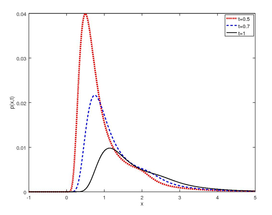
Refer to caption
Figure 4. Left: Solution of the semi-fractional differential equation in Example 5.2 at different times (t=0.5t=0.5, 0.70.7 and 1.01.0). Right: log-log plot of the solution in Example 5.2.
Example 5.2.

Let D1=−1D_{1}=-1, D2=0D_{2}=0, b=5b=5 and T2=1T_{2}=1 such that (5.1) reduces to

∂∂t​p​(x,t)=−∂α∂c,θxα​p​(x,t)for all ​x∈[−5,5],t∈[0,1].\displaystyle\frac{\partial}{\partial t}p(x,t)=-\frac{\partial^{\alpha}}{\partial_{c,\theta}x^{\alpha}}p(x,t)\quad\text{for all }x\in[-5,5],\,t\in[0,1].

In addition, we choose α=0.5\alpha=0.5, c=eπc=e^{\pi} and θ⁡(x)=α​sin⁡(x)+Γ⁡(1−α)\theta(x)=\alpha\sin(x)+\Gamma(1-\alpha). Then θ\theta is a smooth admissable function with respect to cc and α\alpha. Following Remark 5.10 in [15] the solution p1p_{1} of the corresponding fractional equation at time T1=0.01T_{1}=0.01 (our starting point) is given by Sα​(1,σ,0)S_{\alpha}(1,\sigma,0), where σ=(T1​cos⁡(π​α2))1/α\sigma=(T_{1}\cos(\frac{\pi\alpha}{2}))^{1/\alpha}. Starting from p1p_{1} We are now able to approximately calculate the solution of the semi-fractional diffusion equation. In Figure 4 the result is given for different values of t∈[T1,T2]t\in[T_{1},T_{2}] and a log-log plot of the solution shows oscillations about a straight line which can also be seen in practical applications [20].

Refer to caption
Refer to caption
Refer to caption
Refer to caption
Figure 5. Solution of the semi-fractional differential equation in Example 5.3 at different times (t=0.3t=0.3, 0.350.35, 0.40.4 and 0.450.45).
Example 5.3.

Let D1=−0.5=D2D_{1}=-0.5=D_{2}, b=5b=5 and T2=0.45T_{2}=0.45. Again, we choose α=0.5\alpha=0.5 but this time we consider the function θ⁡(x)=α​cos⁡(x)+Γ⁡(1−α)\theta(x)=\alpha\cos(x)+\Gamma(1-\alpha) with c=eπc=e^{\pi}. Then θ\theta is a smooth admissable function with respect to α\alpha and cc. Our starting point is the corresponding stable density at T1=0.01T_{1}=0.01 with representation Sα​(0,σ,0)S_{\alpha}(0,\sigma,0), where σ\sigma is as in Example 5.2. In Figure 5, the numerically calculated semistable density is shown for different values of t∈[T1,T2]t\in[T_{1},T_{2}]. Note that the pictures indicate the appearance of more than one change between convexity and concavity in each of the tails of the semistable densities, which for stable distributions cannot happen. This is also apparent from numerical calculations of one-sided semistable densities by Laplace inversion techniques in [4].

References

  • [1] Andrews, G.E.; Askey, R.; and Roy, R. (1999) Special Functions. Cambridge University Press, Cambridge.
  • [2] Bateman, D.; Eaton, J.W.; Hauberg, S.; and Wehbring, R. (2016) GNU Octave version 4.2.0 manual: a high-level interactive language for numerical computations.
    www.gnu.org/software/octave/doc/interpreter/
  • [3] Bateman, H. (1954) Tables of Integral Transforms, Vol. 1. McGraw-Hill, New York.
  • [4] Chaudhuri, R. (2014) Non-Gaussian Semi-Stable Distributions and Their Statistical Applications. Ph.D. Thesis, University of North Carolina, Chapel Hill.
    cdr.lib.unc.edu/indexablecontent/uuid:a92e2348-bb06-4e0e-9a65-ba8112406df0
  • [5] Chavez, A. (2000) A fractional diffusion equation to describe Lévy flights. Phys. Lett. A 239 13–16.
  • [6] Flajolet, P.; and Sedgewick, R. (2009) Analytic Combinatorics. Cambridge University Press, Cambridge.
  • [7] Folland, G.B. (1992) Fourier Analysis and Its Applications. Wadsworth & Brooks/Cole, London.
  • [8] Hazewinkel, M. ed. (1988) Encyclopaedia of Mathematics, Vol. 1. Reidel, Kluwer, Dordrecht.
  • [9] Huillet, T.; Porzio, A.; and Ben Alaya, M. (2001) On Lévy stable and semistable distributions. Fractals 9 347–364.
  • [10] Kelly, J.F.; Li, C.G.; and Meerschaert, M.M. (2018) Anomalous diffusion with ballistic scaling: A new fractional derivative. J. Comp. Appl. Math. 339 161–178.
  • [11] Kilbas, A.A.; Srivastava, H.M.; and Trujillo, J.J. (2006) Theory and Applications of Fractional Differential Equations. North-Holland Mathematical Studies 204, Elsevier, Amsterdam.
  • [12] Martin-Löf, A. (1985) A limit theorem which clarifies the “Petersburg paradox”. J. Appl. Probab. 22 634–643.
  • [13] Meerschaert, M.M.; and Scheffler, H.P. (2001) Limit Distributions for Sums of Independent Random Vectors. Wiley, New York.
  • [14] Meerschaert, M.M.; and Scheffler, H.P. (2002) Semistable Lévy motion. Fractional Calculus and Applied Analysis 5 27–54.
  • [15] Meerschaert, M.M.; and Sikorskii, A. (2012) Stochastic Models for Fractional Calculus. De Gruyter, Berlin.
  • [16] Meerschaert, M.M.; and Tadjeran, C. (2006) Finite difference approximations for two-sided space-fractional partial differential equations. Appl. Numerical Math. 56 80–90.
  • [17] Metzler, R.; and Klafter, J. (2000) The random walk’s guide to anomalous diffusion: A fractional dynamics approach. Phys. Rep. 339 1–77.
  • [18] Samko, S.G.; Kilbas, A.A.; and Marichev, O.I. (1993) Fractional Integrals and Derivatives. Gordon and Breach, London.
  • [19] Sato, K. (1999) Lévy Processes and Infinitely Divisible Distributions. Cambridge University Press, Cambridge.
  • [20] Sornette, D. (1998) Discrete-scale invariance and complex dimensions. Physics Reports 297 239–270.
  • [21] Sornette, D. (2017) Why Stock Markets Crash: Critical Phenomena in Complex Financial Systems. Princeton University Press, Princeton.