The "Hot Spots" Conjecture on the Vicsek Set
Abstract.
We prove the “hot spots” conjecture on the Vicsek set. Specifically, we will show that every eigenfunction of the second smallest eigenvalue of the Neumann Laplacian on the Vicsek set attains its maximum and minimum on the boundary.
1. Introduction
The “hot spots” conjecture studies whether a flat piece of metal that is given an initial heat distribution will achieve its highest temperatures on its boundary given enough time. That is, the conjecture claims that in a two-dimensional, bounded, connected domain , the heat at point at time , , achieves its maximum value on the boundary of . The “hot spots” conjecture was first posed by Rauch in 1974. An equivalent formulation of the conjecture is as follows: every eigenfunction of the second eigenvalue of the Neumann Laplacian attains its maximum and minimum on the boundary. The conjecture has been shown to be true for some Euclidean domains [1, 2, 3, 4] including recently for thin curved strips [5], but it has also been shown to fail in others [6, 7].
There is now a notion of a Laplacian on many fractals, and the theory of eigenfunctions of the Laplacian is well developed in many cases. Therefore, one can formulate the “hot spot” conjecture on these fractals. We are going to use the theory developed by Kigami [8], see also [9] that applies to the class of post critically finite (p.c.f.) fractals. For many such fractals, eigenvalues and eigenfunctions of the Laplacian can be computed explicitly via a method called spectral decimation [10, 11, 12, 13]. The “hot spots” conjecture has been shown to hold on the Sierpinski gasket and higher dimensional variants [14, 15, 16] but fail on the hexagasket fractal [17]. The hexagasket fractal is determined by an iterated function system consisting of six contractions. However, the analytic boundary in the sense of Kigami studied in [17] consists of only three of the six fixed points of the iterated function system. On the other hand, the boundary of the Sierpinski gasket and its higher dimensional variants mentioned above consists of all of the fixed points of the iterated function system that determines the gasket. Therefore, one might wonder whether the failure of the “hot spots” conjecture on the hexagasket fractal might be due to the “smaller” boundary considered in [17]. The Vicsek set [18, 19, 20] is another type of fractal that has been studied heavily. Zhou [21] described the spectral decimation on a family of Vicsek sets, , in terms of Chebyshev polynomials, and the authors of [22] used Zhou’s formulas to study the Laplacian and spectral operators on the Vicsek set. We study in this paper the Vicsek set that is generated by five contractions; however, its analytic boundary consists of only four of the five fixed points of the iterated function systems. Our main theorem states that, unlike the hexagasket, the “hot spots” conjecture on the Vicsek set is true. The proof of the main theorem is inspired by proofs in [14, 15] and [16]. It is, however, more involved and technical.
The organization of the paper is as follows: the second part of the introduction contains a background on the Vicsek set , and the energy and the Laplacian on the Vicsek set. In section 2, we review the Neumann Laplacian on , and show how to use the spectral decimation to determine the second smallest eigenvalue of the Neumann Laplacian together with a basis of its eigenspace. Section 3 contains our main theorem. The proof of the theorem follows relatively easily from Lemma 3.2 by an argument similar to the one in [14]. The proof of the lemma, however, is very long and technical and occupies the entirety of Section 4. We placed the statement and proof of some formulas used throughout the paper in the Appendix in order to help with the readability of Section 4.
Acknowledgment: This paper grew up from the second’s author project that fulfilled the requirements of the Honors program in the Department of Mathematics at the United States Naval Academy under the supervision of the first author. We thank all the members of the Department that read the Honors project and gave us feedback, especially Professor David Joyner, whose many suggestions led to a much better Honors project and, we hope, a better paper. The authors would also like to thank the anonymous referee and language editor for many useful suggestions that led to an improvement in the presentation of the paper.
1.1. Background
We begin by reviewing several concepts in analysis on fractals as applied to the Vicsek set. First, an iterative function system on a complete metric space is a finite set of contraction mappings , [23, 24]. Given such an iterated function system there exists a unique compact invariant set ; that is, satisfies the following self-similar property,
The main object of study in this paper is the second order Vicsek set, , which is the unique invariant subset of of the iterated function system defined by the following five similarities:
| (1) |
where , , , , and .
A picture of the Vicsek set is provided in the following figure.

The Vicsek set is an example of what in the literature is called a p.c.f fractal and, thus, Kigami’s theory [8] (see also [9]) applies to . We describe next how this theory is applied to the Vicsek set in order to define the standard energy and Laplacian on . A useful feature of the Vicsek is that it can be approximated by an increasing sequence of graphs, as follows: the level zero graph approximation of the Vicsek set, , shown below, consists of the set of vertices at , , , and connected as in a complete graph. Note that , where . The set is also the boundary of the fractal in the sense of [8, 21]. We call the graph 0-cell.

The level 1 graph approximation of the Vicsek set, is constructed as follows: each of the five scaled versions of the level 0 Vicsek set which comprise can be obtained by applying , , etc. Therefore
and, in particular, the set of vertices of equals . We call the sets graph -cells. We note that there are five graph 1-cells.

In the general case, for , the level graph approximation is obtained from the level graph approximation via
The image under the maps of the graph -cells form the graph -cells. We note that each graph -cell contains five graph -cells. That is, when going from level to level , a graph -cell is going to be replaced by five graph -cells. We write as the set of vertices at the level graph approximation. Inductively, it can be shown that , and that is a dense subset of . Thus, it suffices to study continuous functions on and extend them via continuity to .
As detailed by [9], we can define graph energy at level for the Vicsek set as follows:
where means that and are neighboring vertices in (that is, there is an edge in joining and ). Energy generally requires renormalization with a given renormalization factor. For , the renormalization factor is equal to 3 [21]. Thus, for , the renormalized graph energy is . One can define the fractal’s energy, , via
with the domain of the energy, , consisting of all continuous functions on such that . As detailed in [8, 9, 21], the choice of the renormalization constant in the definition of guarantees that the domain of the energy is non-trivial. Now, knowing that the energy exists and can be written as above, we know from [8, 9] that we can determine a fractal’s Laplacian. In dom, extends via the polarization formula to the bilinear function . We consider the standard invariant measure on ; that is, the unique measure that satisfies the following property (see [23] and [24] for details):
Define the weak formulation of the Laplacian as follows ([8, 9]): we say that a function belongs to the domain of the Laplacian if there is a continuous function on such that
for all . In this case we write . As proven in [21], there exists an equivalent pointwise formula for the Laplacian on the Vicsek set. This formula is given as the normalized limit of a series of graph approximations and is written as follows for :
for all not in the boundary . Here the graph Laplacian of the graph , denoted by , is defined by
| (2) |
for all , where represents the number of neighbors of in . The degree of a vertex in is either or for all .
2. Neumann Laplacian and spectral decimation
We study the Neumann Laplacian in this paper. That is, the Laplacian as defined with Neumann boundary conditions. Neumann boundary conditions behave such that Equation (2) holds for all , including the boundary .
The Neumann Laplacian of the level 0 graph approximation for is then given by the following matrix:
The scaling factor outside of the matrix is derived from the that appears in front of the summation in the equation for .
In order to study eigenvalues and eigenfunctions on , we use the process of spectral decimation as described in [9, 21] that we review next. First, there is a local extension algorithm which shows a unique way to extend a function that satisfies the eigenvalue equation on to a function that we still denote by that satisfies the eigenvalue equation on . Moreover there exists a rational function such that = if is not a forbidden eigenvalue. That is, a singularity of the function . It is "forbidden" to decimate to such eigenvalues. Because forbidden eigenvalues do not have a predecessor, i.e. there is no corresponding to , we say that forbidden eigenvalues are "born" at a level of approximation . Spectral decimation for is performed as follows. First, define
| (3) | ||||
where and represent the Chebyshev polynomials of the 1st and 2nd kind, i.e. , , , and . Therefore, , , and . Zhou proved in [21] (see also [9, 22]) that the spectral decimation function is
| (4) |
Additionally, the forbidden eigenvalues of are 4/3 and the zeroes of and , 0, 1/2, and . The extension of eigenfunctions of from one level to the next is given by [22]:
| (5) |
where
Note that and are functions of . Hereafter is any number that is not a forbidden eigenvalue of . In , is equal to the ) adjacency matrix, is the adjacency matrix of () with the degrees of every vertex as its diagonal entries, and is a diagonal matrix such that = -. Going from to , this matrix is applied to the vertices of one graph -cell to obtain the values on the five new graph -subcells.
We follow the convention from [22, Figure 4] when it comes to the labeling of the columns of the matrix (5). That is, the first column corresponds to the point , the second column corresponds to the point , the third column corresponds to , the fourth column corresponds to and so on. To better understand the meaning of the matrix (5), let be an eigenvalue of , and let be a eigenvector on . To simplify the notation, write , . Let be a solution of . Then is extended to a eigenvector on using (5) as described next. First, does not change. The extension of to is computed using the first column of (5) as follows:
where , and are evaluated at . The extension of to is computed using the second column of (5) as follows:
where , and are evaluated at . The computation of the extension of to the remaining vertices in is computed based on the corresponding columns in (5).
The eigenvalue extension function has three local inverses [22]. Let , , denote the inverse functions of in increasing order; that is, is the inverse of on the interval , is the inverse of on , and is the inverse of on . Observe for all in the corresponding domain, and is decreasing while and are increasing. Let be the renormalization factor for the Laplacian. The Neumann eigenvalues are non-negative and they accumulate at . Then the rules for spectral decimation in the case of are summarized as follows [22]:
- (1)
For each Neumann eigenvalue , there is an infinite word , where for all , such that equals
The existence of the limit is proven in [21]. In the first case, the eigenvalue is in the 0-series, and in the second series the eigenvalue is in the 4/3 series born on level
- (2)
All but a finite number of the are equal to 1
- (3)
For the 0-series, the first with must be an odd number, and for the 4/3 series, must be an odd number but
- (4)
The multiplicity of each eigenvalue in the 0-series is 1, while the multiplicity of each 4/3-series eigenvalue on level is .
In the remainder of the paper, we use the spectral decimation as applied to the following setup. Let be the second smallest eigenvalue of . Then has multiplicity 3 and a basis for its eigenspace on is given by the following eigenvectors:
| (6) |
Extend at all levels along . That is, define
| (7) |
and define
| (8) |
We extend and to eigenvectors of on the Vicsek set via the spectral decimation. Figure 4 presents the extension of from to using the spectral decimation described above.

The following important fact follows from [22, Theorem 2.2].
Proposition 2.1.
is the 2nd smallest eigenvalue of the Neumann Laplacian on the Vicsek set.
An important fact later in the paper is that . One can easily check that . The fact that is the smallest preimage of under follows from numerically solving the equation . For future reference, using Maxima approximation, we find that is roughly
3. The "Hot Spots" conjecture for the Vicsek Set
We are now able to state the main theorem. The proof of the theorem follows from the main lemma 3.2. The proof of this lemma is long and technical, and it will occupy the entirety of the next section. Our main result states that every eigenfunction of the second smallest eigenvalue of the Neumann Laplacian on the Vicsek set attains its maximum and minimum on the boundary. Our approach is based on techniques from [14] and [15]. Our computations, however, are much more involved due to the complexity of the spectral decimation matrix (5).
Theorem 3.1 (Main Theorem).
Let be the Vicsek set and be the Neumann Laplacian as described in the previous section. Then every eigenfunction of the second smallest eigenvalue of attains its minimum and maximum value on the boundary .
In order to prove this theorem, we begin by recalling the space of finite words that the five iterated functions (1) of the Vicsek set generate. Let be the corresponding alphabet and let be the set of words of length . Note that in order to simplify the notation we do not separate the letters in a word by commas. So, for example, we write for the word of length 2 that is formed with the letters 1 and 4. Define = as the set of all finite words. For every , we write for the length of . Let denote the empty word and || = 0. Furthermore, = . If then we write for the word obtained by concatenating the two words and together. In particular, we will create words by adding just one letter. For example, is the word that adds the letter at the end of . If all the letters of are the same, say equal to , then we write as , where is the length of .
Recall that where , . We let . For , we write and for we write . Notice that forms a dense subset of .
Recall from (8) that is the second smallest eigenvalue of the Neumann Laplacian where are defined in (7). Recall also that , , and they are related via for all , where is the eigenvalue extension function (4). We let be the the eigenspace of . Then is a three-dimensional vector space by the spectral decimation and we pick the bases given by , , with , , , , , , , , , , , . That is, we pick to be the extensions via the spectral decimation of the -eigenvectors on defined in (6).
Following some ideas from [14], we use the bases that we picked to define a partition of unity on . Specifically, we define the functions and with domain via:
| (9) | ||||
| (10) | ||||
| (11) | ||||
| (12) |
Then they satisfy the following crucial lemma.
Lemma 3.2.
We have and for every and for every . Additionally, , , , where is the Kronecker-Delta function.
As mentioned at the beginning of the section, the proof of the lemma is long, technical, and will occupy the next section of this paper. From the lemma, the theorem is proven as follows.
Proof of Theorem 3.1.
Notice that the functions and are related as follows:
Let . Then there exist constants such that for all because form a basis for . It follows that
Lemma 3.2 implies that the maximum/minimum value of on is given by the maximum/minimum of the values and , which are the values of on the boundary . Since is dense in and is continuous the theorem follows. ∎
4. Proof of Lemma 3.2
The proof of Lemma 3.2 will occupy the rest of this paper. We provide first a short summary of the proof in order to help the reader navigate through the many lemmas that follow. First, an easy proof shows that (Lemma 4.1). We observe that it suffices to prove the statement for for the words that begin only with the letters , and , because restricted to words that begin with and equals a “rotation” of restricted to words that begin with (see Remark 4.4). The crucial Lemma 4.2 proves recursive formulas for when one increases the length of by 1. Using these formulas we are able to compute explicitly for words of the form (Lemma 4.5), (Lemma 4.6), and (Lemma 4.7). Recall that we write for the word of length consisting only on the letter , i.e. (-times). Using these explicit formulas, we prove in Proposition 4.8 that the minimum of is 0 and the maximum of is 1. We finish the proof of Lemma 3.2 by describing how to recover the same results for , and from the results proved for . To improve the readability of this section, we leave the statements and proofs of some useful formulas until the Appendix (see Lemma A.1).
We continue to use the notation described in the previous section. In particular, and are the functions defined in (9), (10), (11), and (12). Recall that we do not separate the letters in a word . Therefore, is the word of length 3 that consists of the letters 1, 2 and 3 (we read this word “one, two, three”, as opposed to “one hundred twenty three”). This word will correspond to the composition .
We break the proof of the main Lemma 3.2 into a series of lemmas. We begin with the easier part.
Lemma 4.1.
, , , , where is the empty word and is the Kronecker-Delta function.
Proof.
From the definition of the functions, it is clear that . Notice that
Hence, . Similar statements hold for and by symmetry, and similar computation shows that the result also holds for . ∎
The hard part that remains is to prove that each of these functions is between 0 and 1. First, we begin by proving that and describe recursive relations satisfied by .
because . So = for all .
For the rest of the paper we write , , , for the elements of the extension matrix (5) evaluated at for all and
| (13) | |||||
| (14) | |||||
| (15) | |||||
| (16) |
Lemma 4.2.
The following formulas hold for all :
| (17) | ||||
| (18) | ||||
| (19) | ||||
| (20) | ||||
| (21) | ||||
| (22) | ||||
| (23) | ||||
| (24) | ||||
Proof.
Let for some . That is, . We prove the case of as follows:
Therefore,
The fact that follows from the fact that the corresponding columns in the extension matrix (5) are identical. Therefore (20) holds. The remaining formulas follow by similar computation. The fact that , , , and follows from the fact that , , and . ∎
As an immediate consequence of Lemma 4.2, we obtain the following.
Lemma 4.3.
Let .
- (1)
If then
and .
- (2)
If then
and .
- (3)
If , then
and .
Remark 4.4.
Using Lemma 4.2 and Lemma 4.3, one can prove inductively the following symmetries (“rotations”) of the function :
- (1)
Let be the permutation that flips 2 and 4, . We denote by its extension to as well. Then for all .
- (2)
Let be the permutation defined by . Then for all and .
We call and “rotations” since, if we view defined on via the projection defined by , then flips around the diagonal going from to , and rotates the 2-cell by and moves it into the 2-cell .
There is a permutation that rotates and moves it into the 2-cell . As a consequence, in the following we will only consider words whose first letter is either or .
We begin by proving that 0 for all . We have already shown that for all , so we now prove that 0 for all . We accomplish this by determining explicit formulas for in the following lemma.
Lemma 4.5.
We have and for all . Therefore for all since for all , and for all .
Proof.
We prove the lemma by induction. First, consider in (17); that is, if then:
by Lemma A.1 and
by Lemma A.1. By plugging in we obtain that and . Assume that the claims holds for . Then, using the induction hypothesis, (13), (15), (17) and Lemma A.1, we obtain:
| which, by factoring out and using the fact that , equals | ||||
| which by replacing with equals | ||||
Hence . Now, by using the induction hypothesis, (14), (16), (21) and Lemma A.1, we obtain
| Next, by using the fact that , we observe that equals | ||||
We simplify next the last parenthesis in the above expression:
Replacing with , we obtain
Hence, since , and after multiplying through the remaining terms and simplifying, we obtain
The induction is now complete and the lemma is proved. ∎
Next, we consider , where . We have already shown that for all , so we now prove that 0 for all .
Lemma 4.6.
We have and for all . Therefore for all since for all . Moreover, for all .
Proof.
We prove the lemma by induction. First, consider in (18) and (22), and, hence, . We obtain
and
Since it follows that
and
Assume now that and that . We prove that and that . Using (22) we have
Then notice from Lemma A.1 that
Therefore,
Factoring out and the denominator we obtain
We now use the following relationship
Therefore,
Finally, notice that
Therefore,
The proof that follows as below:
The induction is now complete and the lemma is proved. ∎
Lemma 4.7.
We have
| (25) |
and
| (26) |
for all . Therefore, is a decreasing sequence and is an increasing sequence. The limit of both of these sequences equals .
Proof.
We begin with . Using (21) we have
where in the last step we used Lemma A.1 and the fact that since .
Using equation (22) we obtain
Since , the equations (22), (23), and (24) imply that . Assume now that (25) and (26) hold for . We prove the induction step:
| which, after we cancel out and , and factor out the products (notice that the 3 in front of reduces the power of 3 in the second product), equals | ||||
where we used Lemma A.1 in the last equality.
Using now equation (22) we obtain
| which, after canceling and , and simplifying the remaining two expressions involving (notice that the expression with a in front of the big product needs to be multiplied by a 3 for the common denominator) equals | ||||
by using Lemma A.1 again. The induction is complete. The last part of the lemma follows from the fact that is a decreasing sequence whose limit is 0 and . In particular, is decreasing to 0. ∎
Thus, 0 for all and . The next step is to prove that for all . We accomplish this by showing that, for a fixed , we have and (where is the word formed by the letter followed by the word ). By Remark 4.4 we only need to prove the statement for , and .
Proposition 4.8.
With the notation as above, we have
and
for all . Therefore, and .
Proof.
We begin by proving the proposition for the case . As noted above, it suffices to consider the cases and . We begin with . Lemma 4.5 implies that and . Moreover, the minimum is attained at , and the maximum is attained at and 4. The second part of Lemma 4.3 with and Lemma 4.5 implies that
and . Recall also that , , , , , , , and . Therefore we only need to check that . Using equation (19) we have
Using (13) we have
Therefore,
since . Therefore,
where we grouped a with to obtain , and we used the proof of Lemma 4.5 to get the last equality. A similar computation shows that
For the last remaining vertex, we use (21). We have
Since , we have . Therefore,
| which, by combining a with , equals | ||||
by the proof of Lemma 4.5. To prove that we modify the above proof as follows:
which using that equals
| Since , by the proof of Lemma 4.5, and by factoring out , equals | ||||
where we used the fact that and the fact that the inequality is clearly true. Therefore .
We move now to the case and . We note that by Lemma 4.6, and . Moreover, the minimum is attained at and 3, and the maximum is attained at . Therefore Lemma 4.6 and the first part of Lemma 4.3 applied to imply that
and . Also, , , , , , , and . Therefore, we only need to check that . We have
It follows that
since and (see Lemma A.1). Hence . Moreover, since (see Lemma A.1), we have by comparing (20) against (21).
Using now equation (24), we obtain
Hence
since and (see Lemma A.1). Hence . Moreover, since it follows that by comparing (24) against (21). So we are done with and .
Next we consider and . We have
and
. Moreover, the
maximum is attained at and the minimum is attained at
and . Therefore, using the last part of Lemma 4.3 we
obtain
and . Moreover, , , and ; all of these values are given by (26) with . We also know the value of from (25). Therefore, we only need to check that the value of is between and . Using (18) we have
Therefore,
| which, since (see Lemma A.1), equals | ||||
by Lemma A.1. Hence . To prove that is smaller than we proceed as follows using (18):
since, by Lemma A.1, and (for we have ). Therefore , and so we proved the statement of the Proposition for .
Moving to , we see that we can repeat the above arguments inductively when increasing the length of from to . This is because, by Lemma 4.2, depends only on the values and . If , then the possible combinations of these values are (see the computations above): three of them are equal to 1 and the fourth equals (by Lemma 4.5); one value is , one value is , and the other two values are between and 1; and three values equal and one value equals . Then the proof given for and can be easily adapted to prove the inductive step.
If , the possible values of and are: three of them equal 0, and one equals ; three of them equal and the fourth one is between and ; and one of the values is for some , and the other three values are between and . Therefore, the arguments given above for and can be easily adapted to these cases to prove the inductive step.
If then the possible values of and : all four are given by Lemma 4.7 and, in particular, three of them are equal; and three of them are equal and all of them are in between the values provided by Lemma 4.7. Then the above argument for and can also be adapted for the induction step on the length of .
Appendix A A few facts used in the proofs
We now collect several relationships and formulas satisfied by and that we used throughout the paper. The proofs of the following statements are straight computations and/or easy calculus problems.
Lemma A.1.
- (1)
The map can be factored out as
and it satisfies the relation
- (2)
The following identities are true for all that are not forbidden values:
- (3)
and for all , and for all . In particular, for all .
- (4)
and .
- (5)
and for all . Therefore and for all .
- (6)
for all .
Proof.
- (1)
The formula for is proved in [22] and follows immediately from its definition.
- (2)
These formulas were also discussed and used in [22].
- (3)
These formulas follow by direct computations. We also used the Maxima CAS [25] to double check our computations. The Maxima code that we used is provided on our website.
- (4)
This can be shown using standard methods of calculus. We provide next pictures that illustrate our claim:

(a) with . 
(b) with . 
(c) with . - (5)
Once again we provide a picture instead of presenting the computation of the derivative of each expression:

(a) with . 
(b) with . - (6)
One more picture to illustrate the last statement:
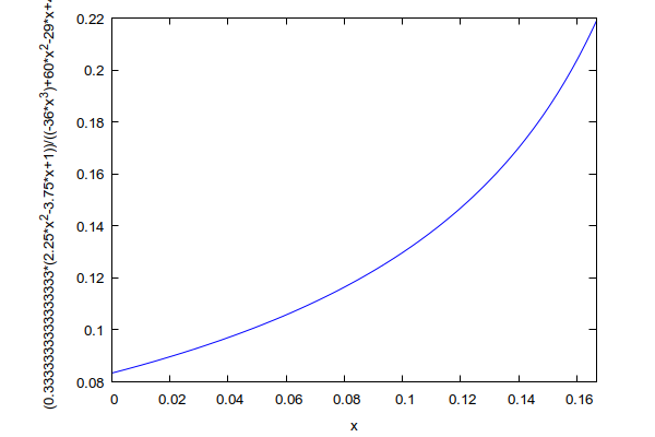
Figure 7. with .
∎
References
- [1] Rodrigo Bañuelos and Krzysztof Burdzy. On the “hot spots” conjecture of J. Rauch. J. Funct. Anal., 164(1):1–33, 1999.
- [2] Rami Atar and Krzysztof Burdzy. On Neumann eigenfunctions in lip domains. J. Amer. Math. Soc., 17(2):243–265, 2004.
- [3] David Jerison and Nikolai Nadirashvili. The “hot spots” conjecture for domains with two axes of symmetry. J. Amer. Math. Soc., 13(4):741–772, 2000.
- [4] Yasuhito Miyamoto. The “hot spots” conjecture for a certain class of planar convex domains. J. Math. Phys., 50(10):103530, 7, 2009.
- [5] David Krejcirik and Matěj Tušek. Location of hot spots in thin curved strips. ArXiv e-prints, September 2017.
- [6] Krzysztof Burdzy and Wendelin Werner. A counterexample to the “hot spots” conjecture. Ann. of Math. (2), 149(1):309–317, 1999.
- [7] Krzysztof Burdzy. The hot spots problem in planar domains with one hole. Duke Math. J., 129(3):481–502, 2005.
- [8] Jun Kigami. Analysis on fractals, volume 143 of Cambridge Tracts in Mathematics. Cambridge University Press, Cambridge, 2001.
- [9] Robert S. Strichartz. Differential equations on fractals. Princeton University Press, Princeton, NJ, 2006. A tutorial.
- [10] R. Rammal and G. Toulouse. Random walks on fractal structures and percolation clusters. J. Phys. Lett., 44(10):L13–L22, 1983.
- [11] Tadashi Shima. On eigenvalue problems for the random walks on the Sierpiński pre-gaskets. Japan J. Indust. Appl. Math., 8(1):127–141, 1991.
- [12] M. Fukushima and T. Shima. On a spectral analysis for the Sierpiński gasket. Potential Anal., 1(1):1–35, 1992.
- [13] Tadashi Shima. On eigenvalue problems for Laplacians on p.c.f. self-similar sets. Japan J. Indust. Appl. Math., 13(1):1–23, 1996.
- [14] Huo-Jun Ruan. The “hot spots” conjecture for the Sierpinski gasket. Nonlinear Anal., 75(2):469–476, 2012.
- [15] Huo-Jun Ruan and Yong-Wen Zheng. The “hot spots” conjecture on the level-3 Sierpinski gasket. Nonlinear Anal., 81:101–109, 2013.
- [16] Xiao-Hui Li and Huo-Jun Ruan. The “hot spots” conjecture on higher dimensional Sierpinski gaskets. Commun. Pure Appl. Anal., 15(1):287–297, 2016.
- [17] Ka-Sing Lau, Xiao-Hui Li, and Huo-Jun Ruan. A Counterexample to the ’Hot Spots’ Conjecture on Nested Fractals. Journal of Fourier Analysis and Applications, pages 1–16, 2016.
- [18] Martin T. Barlow. Diffusions on fractals. In Lectures on probability theory and statistics (Saint-Flour, 1995), volume 1690 of Lecture Notes in Math., pages 1–121. Springer, Berlin, 1998.
- [19] Leonid Malozemov and Alexander Teplyaev. Self-similarity, operators and dynamics. Math. Phys. Anal. Geom., 6(3):201–218, 2003.
- [20] Volker Metz. How many diffusions exist on the Vicsek snowflake? Acta Appl. Math., 32(3):227–241, 1993.
- [21] Denglin Zhou. Spectral analysis of Laplacians on the Vicsek set. Pacific J. Math., 241(2):369–398, 2009.
- [22] Sarah Constantin, Robert S. Strichartz, and Miles Wheeler. Analysis of the Laplacian and spectral operators on the Vicsek set. Commun. Pure Appl. Anal., 10(1):1–44, 2011.
- [23] John E. Hutchinson. Fractals and self-similarity. Indiana Univ. Math. J., 30(5):713–747, 1981.
- [24] Michael F. Barnsley. Fractals everywhere. Academic Press Professional, Boston, MA, second edition, 1993. Revised with the assistance of and with a foreword by Hawley Rising, III.
- [25] Maxima. Maxima, a computer algebra system. version 5.41.0. http://maxima.sourceforge.net/, 2017.