跳到论文正文
W Papers独立论文阅读器 arXiv:1806.05121 论文正文 计算阅读时间 · 0%
引用这篇论文根据当前论文元数据生成,正式投稿前建议核对。


License: arXiv.org perpetual non-exclusive license
arXiv:1806.05121v2 [cs.IT] 18 Jul 2019

Adaptive path interpolation method for sparse systems:
Application to a censored block model

Jean Barbier⋆*    Chun Lam Chan†    Nicolas Macris†
Abstract

Recently a new adaptive path interpolation method has been developed as a simple and versatile scheme to calculate exactly the asymptotic mutual information of Bayesian inference problems defined on dense factor graphs. These include random linear and generalized estimation, sparse superposition codes, or low-rank matrix and tensor estimation. For all these systems, the adaptive interpolation method directly proves that the replica symmetric prediction is exact, in a simple and unified manner. When the underlying factor graph of the inference problem is sparse the replica prediction is considerably more complicated, and rigorous results are often lacking or obtained by rather complicated methods. In this work we show how to extend the adaptive path interpolation method to sparse systems. We concentrate on a Censored Block Model, where hidden variables are measured through a binary erasure channel, for which we fully prove the replica prediction.

†† ⋆\star Quantitative Life Sciences, International Center for Theoretical Physics, Trieste, Italy.
∗* Statistical Physics Laboratory, École Normale Supérieure, Paris, France.
†\dagger Communication Theory Laboratory, École Polytechnique Fédérale de Lausanne, Switzerland.

1 Introduction

Much progress has been achieved recently in Bayesian inference of high dimensional problems. It has been possible to develop rigorous methods in order to derive exact “single letter” variational formulas for the mutual information in the asymptotic limit of the number of variables tending to infinity, when the prior and all hyperparameters of the problem are assumed to be known (this is referred to as the Bayes-optimal setting). Such formulas have often been first conjectured on the basis of the replica and cavity methods of statistical mechanics of disordered spin systems and are also known as “replica symmetric” formulas [1, 2]. Examples where full proofs have been achieved are random linear estimation and compressed sensing [3, 4, 5], learning for single layer networks [6], generalized estimation in multi-layer settings [7, 8], or low-rank matrix and tensor estimation [9, 10, 11, 12, 13]. Invariably, the Guerra-Toninelli interpolation method [14] has been used to derive one-sided bounds (we note that [5] is exceptional and does not seem to rely directly on the same interpolation). For the converse bounds typically other ideas have usually been necessary, such as spatial coupling [9, 3, 4] or the rigorous version of the cavity method [10, 11, 12]. Recently two of us introduced a new interpolation scheme, called adaptive path interpolation method, that allows to derive the replica symmetric formulas in a more straightforward and unified manner [15], [16]. The new method is quite generic once the mean field solution has been identified and is directly applicable when the concentration of the “overlap” can be proved. Roughly speaking in Bayesian inference the “overlap” is the inner product between the random vector to be inferred and the ground truth vector. For models on dense graphs this concentration follows from variants of Ghirlanda-Guerra identities [17] adapted to Bayesian inference combined with the so-called Nishimori identities.

The successes of the adaptive interpolation method have so far been limited to inference models with a dense underlying factor graph. It is therefore desirable to see to what extent the method can be developed when the factor graph is instead sparse. Typical examples of such systems are Low-Density Parity-Check codes, Low-Density Generator-Matrix (LDGM) codes, or the Stochastic and Censored Block Models. It is fair to say that the replica symmetric formulas for the mutual information is much more complicated in such models. Indeed, besides the measurements (or channel outputs): (i) the sparse graph is also random; (ii) the single letter variational problem involves a functional over a set of probability distributions (instead of scalars as in the dense graph case). Existing rigorous derivations of the replica formulas have so far been achieved using a combination of the interpolation method (first developed by [18] for sparse models) and spatial coupling [19] or the rigorous version of the cavity method [20, 21].

In this work we consider a simple version of the Censored Block Model [22, 23, 24, 25], for which we fully develop the adaptive interpolation method. We believe that this constitutes a first step towards an analysis of more complicated models via this method. A summary of the present analysis was presented in [26].

In the Censored Block Model one has a set of nn hidden binary variables. One observes α​n\alpha n products of random KK-tuples, where α>0\alpha>0 is called the fraction of measurements, through a noisy channel. The goal is to reconstruct an estimate of the hidden variables from the noisy observations. There are other interpretations of this model. For example, it can be interpreted as a Low-Density Generator-Matrix code ensemble, with design communication rate 1/α1/\alpha, on a factor graph with degree KK factor nodes and variable nodes with Poisson degrees (when n→+∞n\to+\infty). Another possible interpretation is, as a model of statistical mechanics, namely an Ising model on a sparse random graph with KK-spin interactions. The Censored Block Model has been discussed when the measurement channel is a Binary Symmetric Channel in [22] and the replica formula proven in this case [21]. Here, we consider a simpler situation where the measurement channel is the Binary Erasure Channel (BEC) for which the adaptive interpolation method can be completely developed. As we will see this method requires concentration results for a whole set of suitable “overlaps” and requires new ideas in the case of sparse graphs. Here, we solve this issue for the BEC, and it is currently the only aspect of the method that is missing for extending our analysis to other channels.

The paper is organized as follows. In Section 2 we give a precise formulation of the model and state the main result of this paper (Theorem 2.3). In Section 3 we review two important tools used throughout our analysis, namely the Nishimori identities and the Griffiths-Kelly-Sherman inequalities. The adaptive interpolation method for the sparse graph models is formulated in Section 4 and the core of the proof of Theorem 2.3 is also developed. This section contains the main new technical ideas of this paper. Overlap concentration is proved in Section 6 and 7. A series of more technical results are found in Section 8 and in the appendices.

2 Setting and main result

2.1 Censored Block Model

We shall denote binary variables by σi∈{−1,+1}\sigma_{i}\in\{-1,+1\}, i=1,…,ni=1,\ldots,n and vectors of such variables by σ¯=(σ1,…,σn)∈{−1,+1}n\underline{\sigma}=(\sigma_{1},\ldots,\sigma_{n})\in\{-1,+1\}^{n}. Subsets S⊂{1,…,n}S\subset\{1,\ldots,n\} with at least two elements are always denoted by capital letters. For the product of binary variables in a subset SS we use the shorthand notation σS≡∏i∈Sσi\sigma_{S}\equiv\prod_{i\in S}\sigma_{i}. If there is a possible confusion between small and capital letter subscripts we occasionally use more specific notations. Below, the integer K≥2K\geq 2 and the fraction α∈ℝ+\alpha\in\mathbb{R}_{+} are fixed independent of nn.

In the Censored Block Model considered in this paper nn hidden binary variables σ¯0=(σ10,…,σn0)\underline{\sigma}^{0}=(\sigma_{1}^{0},\ldots,\sigma_{n}^{0}) are i.i.d. uniform, i.e. drawn independently according to a Ber⁡(1/2){\rm Ber}(1/2) prior P0​(σi0)=12​δσi0,+1+12​δσi0,−1P_{0}(\sigma_{i}^{0})=\frac{1}{2}\delta_{\sigma_{i}^{0},+1}+\frac{1}{2}\delta_{\sigma_{i}^{0},-1}. A noiseless measurement consists in a product σa10​σa20​…​σaK0\sigma_{a_{1}}^{0}\sigma_{a_{2}}^{0}\ldots\sigma_{a_{K}}^{0} of a KK-tuple of variables drawn uniformly at random. The KK-tuple is identified with a subset A≡{a1,…,aK}⊂{1,…,n}A\equiv\{a_{1},\ldots,a_{K}\}\subset\{1,\ldots,n\} and we set σA0≡σa10​σa20​…​σaK0\sigma_{A}^{0}\equiv\sigma_{a_{1}}^{0}\sigma_{a_{2}}^{0}\ldots\sigma_{a_{K}}^{0}. Of course σA0=±1\sigma_{A}^{0}=\pm 1. The true observations JA∈ℝJ_{A}\in\mathbb{R} are noisy versions of these products obtained through a binary input memoryless channel described by some transition probability Q⁡(JA|σA0)Q(J_{A}|\sigma_{A}^{0}). For large nn the total number of observations mm asymptotically follows a Poisson distribution with mean α​n\alpha n, i.e., m∼Poi⁡(α​n)m\sim\mathrm{Poi}(\alpha n). We shall also index the observations as A=1,…,mA=1,\ldots,m.

Let us now describe the Bayesian setting used here to determine the information theoretic limits for reconstructing the hidden variables. From the Bayes rule we have that the posterior given the observations is

P⁡(σ¯|J¯)=∏i=1nP0​(σi)​∏A=1mQ⁡(JA|σA)∑σ¯∈{−1,+1}n∏i=1nP0​(σi)​∏A=1mQ⁡(JA|σA).\displaystyle P(\underline{\sigma}|\underline{J})=\frac{\prod_{i=1}^{n}P_{0}(\sigma_{i})\prod_{A=1}^{m}Q(J_{A}|\sigma_{A})}{\sum_{\underline{\sigma}\in\{-1,+1\}^{n}}\prod_{i=1}^{n}P_{0}(\sigma_{i})\prod_{A=1}^{m}Q(J_{A}|\sigma_{A})}.

Dividing both the numerator and denominator by ∏A=1mQ⁡(JA|σA=+1)\prod_{A=1}^{m}Q(J_{A}|\sigma_{A}=+1), the posterior P⁡(σ¯|J¯)P(\underline{\sigma}|\underline{J}) can be rewritten as

P⁡(σ¯|J¯~)=1𝒵​exp​∑A=1mJ~A​(σA−1),\displaystyle P(\underline{\sigma}|\underline{\tilde{J}})=\frac{1}{\cal Z}\exp\sum_{A=1}^{m}\tilde{J}_{A}(\sigma_{A}-1), (1)

where

J~A\displaystyle\tilde{J}_{A} ≡12​ln⁡Q⁡(JA|+1)Q⁡(JA|−1),\displaystyle\equiv\frac{1}{2}\ln\frac{Q(J_{A}|+1)}{Q(J_{A}|-1)},
𝒵\displaystyle{\cal Z} ≡∑σ¯∈{−1,+1}nexp∑A=1mJ~A(σA−1).\displaystyle\equiv\sum_{\underline{\sigma}\in\{-1,+1\}^{n}}\exp\sum_{A=1}^{m}\tilde{J}_{A}(\sigma_{A}-1).

We will use the language and notations of statistical mechanics. The normalization 𝒵{\cal Z} shall be called the partition function. The bipartite factor graph 𝒢\mathcal{G} underlying (1) contains variable nodes i=1,…,ni=1,\ldots,n and constraint (or factor) nodes A=1,…,mA=1,\ldots,m. Each variable node ii “carries” the binary variable σi\sigma_{i} and each constraint node AA “carries” the half-log-likelihood ratio J~A\tilde{J}_{A} and uniformly connects to KK variable nodes a1,…,aKa_{1},\ldots,a_{K}. As said before, we identify A≡{a1,…,aK}A\equiv\{a_{1},\ldots,a_{K}\}. Distribution (1) can be interpreted as the Gibbs distribution of a random spin system (or spin glass). The expectation of a quantity A⁡(σ¯)A(\underline{\sigma}) with respect to the posterior (1) will be denoted by a Gibbs bracket

⟨A⁡(σ¯)⟩≡∑σ∈{−1,+1}nA⁡(σ¯)​P​(σ¯|J¯~).\langle A(\underline{\sigma})\rangle\equiv\sum_{\sigma\in\{-1,+1\}^{n}}A(\underline{\sigma})P(\underline{\sigma}|\underline{\tilde{J}})\,.

The posteroior distribution as well as the expectations ⟨A⁡(σ)⟩\langle A(\sigma)\rangle are random because of the randomness in: OPENi)i) the factor graph 𝒢\mathcal{G} ensemble; OPENi​i)ii) the observations J¯\underline{J} given the hidden vector σ¯0\underline{\sigma}^{0}; and OPENi​i​i)iii) the hidden vector σ¯0\underline{\sigma}^{0}.

It is equivalent to work in terms of observations J¯\underline{J} or associated half-log-likelihood ratios J¯~\underline{\tilde{J}}. The latter are (formally) distributed according to

∏i=1nP0​(σi0)​∏A=1m𝖼⁡(J~A|σA0)​d​J~A≡∏i=1nP0​(σi0)​∏A=1mQ⁡(JA|σA0)​d​JA.\displaystyle\prod_{i=1}^{n}P_{0}({\sigma}^{0}_{i})\prod_{A=1}^{m}\mathsf{c}(\tilde{J}_{A}|\sigma_{A}^{0})d\tilde{J}_{A}\equiv\prod_{i=1}^{n}P_{0}({\sigma}^{0}_{i})\prod_{A=1}^{m}Q(J_{A}|\sigma_{A}^{0})dJ_{A}. (2)

Most of the time it will be more convenient for us to refer directly to half-log-likelihood ratios. The graph, the observations and the hidden vector are called quenched random variables (r.v.) because given instance of the problem their realization is fixed. In contrast the r.v. σ¯\underline{\sigma} is sampled from the posterior (1), and hence is often called an annealed variable. Expectations with respect to the quenched variables are denoted 𝔼𝒢\mathbb{E}_{\mathcal{G}} and 𝔼σ¯0​𝔼J¯~|σ¯0\mathbb{E}_{\underline{\sigma}^{0}}\mathbb{E}_{\underline{\tilde{J}}|\underline{\sigma}^{0}}. To alleviate notations we shall often simply use 𝔼\mathbb{E} when the expectation is taken with respoect to all quenched r.v in the ensuing expression. The bracket ⟨−⟩\langle-\rangle is reserved for expectations with respect to the posterior (1).

Let H(σ¯|J¯~)≡−∑σ¯∈{−1,+1}nP(σ¯|J¯~)lnP(σ¯|J¯~)H(\underline{\sigma}|\underline{\tilde{J}})\equiv-\sum_{{\underline{\sigma}}\in\{-1,+1\}^{n}}P(\underline{\sigma}|\underline{\tilde{J}})\ln P(\underline{\sigma}|\underline{\tilde{J}}) be the conditional entropy of the hidden variables given fixed observations. It is easy to see that the average conditional entropy (per variable) is given by the average free entropy (the r.h.s of the formula)

1n​𝔼𝒢​𝔼σ¯0​𝔼J¯~|σ¯0​H​(σ¯|J¯~)=1n​𝔼𝒢​𝔼σ¯0​𝔼J¯~|σ¯0​ln⁡𝒵.\displaystyle\frac{1}{n}\mathbb{E}_{\mathcal{G}}\mathbb{E}_{\underline{\sigma}^{0}}\mathbb{E}_{\underline{\tilde{J}}|\underline{\sigma}^{0}}H(\underline{\sigma}|\underline{\tilde{J}})=\frac{1}{n}\mathbb{E}_{\mathcal{G}}\mathbb{E}_{\underline{\sigma}^{0}}\mathbb{E}_{\underline{\tilde{J}}|\underline{\sigma}^{0}}\ln{\cal Z}. (3)

We refer readers to [27] for details. The singularities, as a function of the measurement fraction α\alpha, of this limiting quantity when n→+∞n\to+\infty give us the information theoretic thresholds, or the location of static phase transitions in physics language.

2.2 The replica symmetric formula for the average conditional entropy

The cavity method [1] predicts that the asymptotic average conditional entropy per variable is accessible from the following “replica symmetric” functional. This functional is an “average form” of the Bethe free entropy expression. Details of the relationship between the replica symmetric functional and Bethe free entropy can be found in [28, Appendix VII].

Definition 2.1 (The replica symmetric free entropy functional).

Let VV be a r.v. with distribution 𝗑\mathsf{x}, and ViV_{i}, i=1,…,Ki=1,\ldots,K i.i.d. copies of VV. Let11 1 Equation (4) corresponds to one of the two density evolution fixed point equations associated with the belief propagation algorithm, see [2] for the links between this algorithm and the replica symmetric functional.

U\displaystyle U =tanh−1⁡(tanh⁡J~​∏i=1K−1tanh⁡Vi),\displaystyle=\tanh^{-1}\Big(\tanh\tilde{J}\prod_{i=1}^{K-1}\tanh V_{i}\Big), (4)

and UBU_{B}, B=1,…,lB=1,\ldots,l i.i.d. copies of UU where l∼Poi⁡(α​K)l\sim\mathrm{Poi}(\alpha K) is a Poisson distributed integer. Let σ0∼P0\sigma^{0}\sim P_{0} and ∏a=1Kσa\prod_{a=1}^{K}\sigma_{a} be the product of KK independent copies. Let J~∼𝖼⁡(J~|∏a=1Kσa)\tilde{J}\sim\mathsf{c}(\tilde{J}|\prod_{a=1}^{K}\sigma_{a}) (see equation (2)). The replica symmetric free entropy functional is defined to be

hRS(𝗑)≡𝔼l𝔼σ1,⋯,σK𝔼J~|∏a=1Kσa𝔼U¯𝔼V¯[\displaystyle{h}_{\mathrm{RS}}(\mathsf{x})\equiv\mathbb{E}_{l}\mathbb{E}_{\sigma_{1},\cdots,\sigma_{K}}\mathbb{E}_{\tilde{J}|\prod_{a=1}^{K}\sigma_{a}}\mathbb{E}_{\underline{U}}\mathbb{E}_{\underline{V}}\Big[ ln⁡(∏B=1l(1+tanh⁡UB)+∏B=1l(1−tanh⁡UB))\displaystyle\ln\Big(\prod_{B=1}^{l}(1+\tanh U_{B})+\prod_{B=1}^{l}(1-\tanh U_{B})\Big)
−α(K−1)ln(1+tanhJ~∏i=1KtanhVi)−αln(1+tanhJ~)].\displaystyle-\alpha(K-1)\ln\Big(1+\tanh\tilde{J}\prod_{i=1}^{K}\tanh V_{i}\Big)-\alpha\ln(1+\tanh\tilde{J})\Big]. (5)
Remark 2.2.

For uniform P0P_{0} we can replace the product ∏a=1Kσa\prod_{a=1}^{K}\sigma_{a} by a single binary variable σ0∼P0\sigma_{0}\sim P_{0}.

While a substantial part of our analysis holds for general (symmetric) memoryless channels, our main result is fully proved for the BEC. This channel has transition probability

Q⁡(JA|σA0)=(1−q)​δJA,σA0+q​δJA,0,Q(J_{A}|\sigma_{A}^{0})=(1-q)\delta_{J_{A},\sigma_{A}^{0}}+q\delta_{J_{A},0}\,,

and from (2) we get in this case

𝖼⁡(J~A|σA0)=(1−q)​δσA0​J~A,+∞+q​δJ~A,0.\mathsf{c}(\tilde{J}_{A}|\sigma_{A}^{0})=(1-q)\delta_{\sigma_{A}^{0}\tilde{J}_{A},+\infty}+q\delta_{\tilde{J}_{A},0}\,.

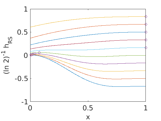
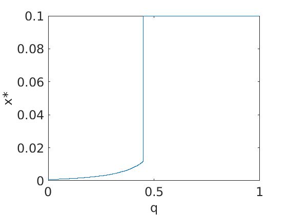
The set of distributions with point masses at {0,+∞}\{0,+\infty\} plays a special role and will be called ℬ\mathcal{B}. We adopt the notation (from coding theory) Δ0\Delta_{0} and Δ∞\Delta_{\infty} for the two point masses at 00 and +∞+\infty. Any distribution 𝗑∈ℬ\mathsf{x}\in\mathcal{B} is of the from 𝗑=x​Δ0+(1−x)​Δ∞\mathsf{x}=x\Delta_{0}+(1-x)\Delta_{\infty}, with x∈[0,1]x\in[0,1]. In this case the replica symmetric free entropy functional becomes (5) becomes a function of x∈[0,1]x\in[0,1]. A numerical illustration is found in Appendix F.

Our main result is the proof, through the use of the adaptive interpolation method for sparse graphs, of the following theorem:

Theorem 2.3 (The replica symmetric formula is exact for the BEC channel).

For a Censored Block Model with observations obtained through a Binary Erasure Channel as described above we have

limn→∞1n​𝔼𝒢​𝔼σ¯0​𝔼J¯~|σ¯0​H​(σ¯|J¯~)=sup𝗑∈ℬhRS​(𝗑).\displaystyle\lim_{n\rightarrow\infty}\frac{1}{n}\mathbb{E}_{\mathcal{G}}\mathbb{E}_{\underline{\sigma}^{0}}\mathbb{E}_{\underline{\tilde{J}}|\underline{\sigma}^{0}}H(\underline{\sigma}|\underline{\tilde{J}})=\sup_{\mathsf{x\in\mathcal{B}}}\ h_{\mathrm{RS}}(\mathsf{x}). (6)

This theorem is a direct consequence of two main Propositions 4.5 and 4.12 proved in Sec. 4.

3 Two preliminary tools

In this section we review standard material which is needed in our analysis. For more details the reader can consult [29, 30, 31]

3.1 Nishimori identities

3.1.1 A consequence of Bayes rule

Consider the quantity ∏S∈𝒞σS0​∏S∈𝒞⟨σS⟩\prod_{S\in\mathcal{C}}\sigma_{S}^{0}\prod_{S\in\mathcal{C}}\langle\sigma_{S}\rangle for a given graph and any collection 𝒞\mathcal{C} of subsets S⊂{1,…,n}S\subset\{1,\ldots,n\}. The same subset can occur many times in a collection. From Bayes formula, for a given factor graph 𝒢\mathcal{G},

𝔼σ¯0​𝔼J¯~|σ¯0​[∏S∈𝒞σS0​∏S∈𝒞⟨σS⟩]\displaystyle\mathbb{E}_{\underline{\sigma}^{0}}\mathbb{E}_{\underline{\tilde{J}}|\underline{\sigma}^{0}}\Big[\prod_{S\in\mathcal{C}}\sigma_{S}^{0}\prod_{S\in\mathcal{C}}\langle\sigma_{S}\rangle\Big] =𝔼J¯~​𝔼σ¯0|J¯~​[∏S∈𝒞σS0​∏S∈𝒞⟨σS⟩]\displaystyle=\mathbb{E}_{\underline{\tilde{J}}}\mathbb{E}_{\underline{\sigma}^{0}|\underline{\tilde{J}}}\Big[\prod_{S\in\mathcal{C}}\sigma_{S}^{0}\prod_{S\in\mathcal{C}}\langle\sigma_{S}\rangle\Big]
=𝔼J¯~​[⟨∏S∈𝒞σS⟩​∏S∈𝒞⟨σS⟩]\displaystyle=\mathbb{E}_{\underline{\tilde{J}}}\Big[\langle\prod_{S\in\mathcal{C}}\sigma_{S}\rangle\prod_{S\in\mathcal{C}}\langle\sigma_{S}\rangle\Big]
=𝔼σ¯0​𝔼J¯~|σ¯0​[⟨∏S∈𝒞σS⟩​∏S∈𝒞⟨σS⟩].\displaystyle=\mathbb{E}_{\underline{\sigma}^{0}}\mathbb{E}_{\underline{\tilde{J}}|\underline{\sigma}^{0}}\Big[\langle\prod_{S\in\mathcal{C}}\sigma_{S}\rangle\prod_{S\in\mathcal{C}}\langle\sigma_{S}\rangle\Big]. (7)

The equality between the l.h.s and the last line on the r.h.s is a trivial but very important consequence of Bayes rule. This formula has been abusively called a “Nishimori identity” in the literature. The “true” Nishimori identity is obtained when two extra features are present, namely a “gauge invariance” of the posterior and channel symmetry.

3.1.2 Nishimori identities for symmetric channels

For symmetric channels this identity can be further specialized and yields the so-called Nishimori identities. This is specially important for us since the BEC is a symmetric channel. By definition, symmetric channels are those satisfying Q⁡(JA|σA0)=Q⁡(−JA|−σA0)Q(J_{A}|\sigma_{A}^{0})=Q(-J_{A}|-\sigma_{A}^{0}) or equivalently 𝖼⁡(J~A|σA0)=𝖼⁡(−J~A|−σA0)\mathsf{c}(\tilde{J}_{A}|\sigma_{A}^{0})=\mathsf{c}(-\tilde{J}_{A}|-\sigma_{A}^{0}).

Given σ¯0\underline{\sigma}^{0} the Gibbs distribution (1) is invariant under the gauge transformation σi→σi0​σi\sigma_{i}\to\sigma_{i}^{0}\sigma_{i}, J~A→σA0​J~A\tilde{J}_{A}\to\sigma_{A}^{0}\tilde{J}_{A}. Let us denote by σ¯0⋆J¯~\underline{\sigma}^{0}\star\underline{\tilde{J}} the “component-wise” product (σA0​J~A)A=1m(\sigma_{A}^{0}\tilde{J}_{A})_{A=1}^{m}. Now we perform a gauge transformation on both sides of (7). For the left hand side we have

𝔼J¯~|σ¯0​[∏S∈𝒞σS0​∏S∈𝒞⟨σS⟩]=𝔼σ¯0⋆J¯~|σ¯0​[∏S∈𝒞⟨σS⟩].\displaystyle\mathbb{E}_{\underline{\tilde{J}}|\underline{\sigma}^{0}}\Big[\prod_{S\in\mathcal{C}}\sigma_{S}^{0}\prod_{S\in\mathcal{C}}\langle\sigma_{S}\rangle\Big]=\mathbb{E}_{\underline{\sigma}^{0}\star\underline{\tilde{J}}|\underline{\sigma}^{0}}\Big[\prod_{S\in\mathcal{C}}\langle\sigma_{S}\rangle\Big]. (8)

Moreover, from 𝖼⁡(J~A|σA0)=𝖼⁡(−J~A|−σA0)\mathsf{c}(\tilde{J}_{A}|\sigma_{A}^{0})=\mathsf{c}(-\tilde{J}_{A}|-\sigma_{A}^{0}) one can see that for a symmetric channel 𝖼⁡(σA0​J~A|σA0)=𝖼⁡(J~A|1)\mathsf{c}(\sigma_{A}^{0}\tilde{J}_{A}|\sigma_{A}^{0})=\mathsf{c}(\tilde{J}_{A}|1), and therefore in (8) we can replace 𝔼σ¯0⋆J¯~|σ¯0\mathbb{E}_{\underline{\sigma}^{0}\star\underline{\tilde{J}}|\underline{\sigma}^{0}} by 𝔼J¯~|1¯\mathbb{E}_{\underline{\tilde{J}}|\underline{1}}. We get

𝔼J¯~|σ¯0​[∏S∈𝒞σS0​∏S∈𝒞⟨σS⟩]=𝔼J¯~|1¯​[∏S∈𝒞⟨σS⟩].\displaystyle\mathbb{E}_{\underline{\tilde{J}}|\underline{\sigma}^{0}}\Big[\prod_{S\in\mathcal{C}}\sigma_{S}^{0}\prod_{S\in\mathcal{C}}\langle\sigma_{S}\rangle\Big]=\mathbb{E}_{\underline{\tilde{J}}|\underline{1}}\Big[\prod_{S\in\mathcal{C}}\langle\sigma_{S}\rangle\Big]. (9)

The same steps show that the right hand side of (7) also satisfies

𝔼J¯~|σ¯0​[⟨∏S∈𝒞σS⟩​∏S∈𝒞⟨σS⟩]=𝔼J¯~|1¯​[⟨∏S∈𝒞σS⟩​∏S∈𝒞⟨σS⟩].\displaystyle\mathbb{E}_{\underline{\tilde{J}}|\underline{\sigma}^{0}}\Big[\langle\prod_{S\in\mathcal{C}}\sigma_{S}\big\rangle\prod_{S\in\mathcal{C}}\langle\sigma_{S}\rangle\Big]=\mathbb{E}_{\underline{\tilde{J}}|\underline{1}}\Big[\big\langle\prod_{S\in\mathcal{C}}\sigma_{S}\big\rangle\prod_{S\in\mathcal{C}}\langle\sigma_{S}\rangle\Big]. (10)

From (9), (10), (7) we get the final Nishimori identity

𝔼J¯~|1¯​[∏S∈𝒞⟨σS⟩]=𝔼J¯~|1¯​[⟨∏S∈𝒞σS⟩​∏S∈𝒞⟨σS⟩].\displaystyle\mathbb{E}_{\underline{\tilde{J}}|\underline{1}}\Big[\prod_{S\in\mathcal{C}}\langle\sigma_{S}\rangle\Big]=\mathbb{E}_{\underline{\tilde{J}}|\underline{1}}\Big[\big\langle\prod_{S\in\mathcal{C}}\sigma_{S}\big\rangle\prod_{S\in\mathcal{C}}\langle\sigma_{S}\rangle\Big]. (11)

3.1.3 A special Nishimori identity for symmetric distributions

An important role is played by the space 𝒳\mathcal{X} of symmetric distributions which we define as follows. Take a transition probability (a “channel”) satisfying q⁡(J|σ0)=q⁡(−J|−σ0)q(J|\sigma^{0})=q(-J|-\sigma^{0}), σ0∈{−1,+1}\sigma^{0}\in\{-1,+1\}, J∈ℝJ\in\mathbb{R}. The associated half-log-likelihood variable is h=12​ln⁡q⁡(J|+1)q⁡(J|−1)h=\frac{1}{2}\ln\frac{q(J|+1)}{q(J|-1)}. The space 𝒳\mathcal{X} is the space of symmetric distributions over the half-log-likelihood variable is formally defined by 𝗑⁡(d​h)=q⁡(J|+1)​d​J\mathsf{x}(dh)=q(J|+1)dJ. It is easy to deduce from q⁡(J|σ0)=q⁡(−J|−σ0)q(J|\sigma^{0})=q(-J|-\sigma^{0}) that a symmetric distribution 𝗑∈𝒳\mathsf{x}\in\mathcal{X} satisfies 𝗑⁡(−d​h)=e−2​h​𝗑​(d​h)\mathsf{x}(-dh)=e^{-2h}\mathsf{x}(dh). We note that ℬ⊂𝒳\mathcal{B}\subset\mathcal{X} (recall ℬ\mathcal{B} is the set of convex combinations of point masses at 00 and +∞+\infty).

There is an important special case of the Nishimori identity (11). Namely the one satisfied by the system constituted by a single uniform hidden variable σ0∼P0\sigma^{0}\sim P_{0}, observed through a noisy “channel” q⁡(J|σ0)q(J|\sigma^{0}). The Gibbs distribution is simply in this case eh​σ/(2​cosh⁡h)e^{h\sigma}/(2\cosh h) where hh is the half-log-likelihood of the “channel”. Since ⟨σ⟩=tanh⁡h\langle\sigma\rangle=\tanh h, an application of (11) (where the singleton set is taken kk times) yields

∫(tanh⁡h)2​k−1​𝗑​(𝑑h)=∫(tanh⁡h)2​k​𝗑​(𝑑h),k∈ℕ∗.\displaystyle\int(\tanh h)^{2k-1}\,\mathsf{x}(dh)=\int(\tanh h)^{2k}\,\mathsf{x}(dh),\qquad k\in\mathbb{N}^{*}. (12)

In Appendix A we show in an independent and direct way that any 𝗑∈𝒳\mathsf{x}\in\mathcal{X} satisfies (12).

3.1.4 Conditional entropy for symmetric channels

Since the Gibbs distribution is invariant under a gauge transformation, the partition function 𝒵{\cal Z} also is, and therefore, for a given graph 𝒢\mathcal{G} and hidden vector σ¯0\underline{\sigma}^{0}, we have

𝔼J¯~|σ¯0​ln⁡𝒵\displaystyle\mathbb{E}_{\underline{\tilde{J}}|\underline{\sigma}^{0}}\ln{\cal Z} =𝔼σ¯0⋆J¯~|σ¯0​ln⁡𝒵.\displaystyle=\mathbb{E}_{\underline{\sigma}^{0}\star\underline{\tilde{J}}|\underline{\sigma}^{0}}\ln{\cal Z}. (13)

For symmetric channels the r.h.s. equals 𝔼J¯~|1¯​ln⁡𝒵\mathbb{E}_{\underline{\tilde{J}}|\underline{1}}\ln{\cal Z} and thus the average conditional entropy (3) becomes

1n​𝔼𝒢​𝔼σ¯0​𝔼J¯~|σ¯0​H​(σ¯|J¯~)=1n​𝔼𝒢​𝔼J¯~|1¯​ln⁡𝒵.\displaystyle\frac{1}{n}\mathbb{E}_{\mathcal{G}}\mathbb{E}_{\underline{\sigma}^{0}}\mathbb{E}_{\underline{\tilde{J}}|\underline{\sigma}^{0}}H(\underline{\sigma}|\underline{\tilde{J}})=\frac{1}{n}\mathbb{E}_{\mathcal{G}}\mathbb{E}_{\underline{\tilde{J}}|\underline{1}}\ln{\cal Z}. (14)

3.1.5 Summary

When one is dealing with symmetric measurement channels, in order to compute the average conditional entropy, or certain averages, one may assume that σi0=1\sigma_{i}^{0}=1, i=1,…,ni=1,\ldots,n and that the quenched variables J¯~\underline{\tilde{J}} have distribution 𝖼⁡(J~A|1)\mathsf{c}(\tilde{J}_{A}|1), A=1,…,mA=1,\ldots,m. From now on this is understood unless explicitly specified otherwise.

3.2 Griffiths-Kelly-Sherman inequalities for the BEC

The BEC is a symmetric channel so as shown before, without loss of generality for analysis purposes, we assume σi0=1\sigma_{i}^{0}=1, i=1,…,ni=1,\ldots,n and that J¯~\underline{\tilde{J}} have distribution 𝖼⁡(J~A|1)\mathsf{c}(\tilde{J}_{A}|1), A=1,…,mA=1,\ldots,m. Since 𝖼⁡(J~A|1)=(1−q)​Δ∞+q​Δ0\mathsf{c}(\tilde{J}_{A}|1)=(1-q)\Delta_{\infty}+q\Delta_{0} the Gibbs distribution (1) has non-negative coupling constants J~A\tilde{J}_{A}, A=1,…,mA=1,\ldots,m. Therefore the Gibbs distribution satisfies the Griffiths-Kelly-Sherman (GKS) inequalities [32, 29, 30]: For any subsets of variable indices S,T⊂{1​…​n}S,T\subset\{1\ldots n\} we have

⟨σS⟩≥0,\displaystyle\langle\sigma_{S}\rangle\geq 0, (15)
⟨σS​σT⟩−⟨σS⟩​⟨σT⟩≥0.\displaystyle\langle\sigma_{S}\sigma_{T}\rangle-\langle\sigma_{S}\rangle\langle\sigma_{T}\rangle\geq 0. (16)

These two inequalities play an important role in the proof of Theorem 2.3.

4 The adaptive path interpolation method

For t=1,…,Tt=1,\dots,T let Vi(t)V^{(t)}_{i} be i.i.d. r.v. distributed according to 𝗑(t)∈𝒳\mathsf{x}^{(t)}\in\mathcal{X}. Consider the r.v.

U(t)=tanh−1⁡(tanh⁡J~​∏i=1K−1Vi(t))\displaystyle U^{(t)}=\tanh^{-1}\Big(\tanh\tilde{J}\prod_{i=1}^{K-1}V_{i}^{(t)}\Big) (17)

and independent copies denoted UB(t)U^{(t)}_{B} where BB is a subscript which runs over l(t)∼Poi⁡(KR​T)l^{(t)}\sim\mathrm{Poi}(\frac{K}{RT}) of these copies. Later on, we call 𝗑~(t)\tilde{\mathsf{x}}^{(t)} the distribution of U(t)U^{(t)} (induced by 𝗑(t)\mathsf{x}^{(t)} and 𝖼\mathsf{c}).

Let also define two extra random variables, HH with distribution ϵ​Δ∞+(1−ϵ)​Δ0∈ℬ\epsilon\Delta_{\infty}+(1-\epsilon)\Delta_{0}\in\mathcal{B}, and H~\tilde{H} with distribution δ​n−θ​Δ∞+(1−δ​n−θ)​Δ0∈ℬ\delta n^{-\theta}\Delta_{\infty}+(1-\delta n^{-\theta})\Delta_{0}\in\mathcal{B}, where ϵ,δ∈(0,1)\epsilon,\delta\in(0,1) and θ∈(0,1)\theta\in(0,1) (eventually we will have to take θ∈(0,1/5]\theta\in(0,1/5] in the final estimates).

Let us set 𝗑¯=(𝗑(1),…,𝗑(T))\underline{\mathsf{x}}=(\mathsf{x}^{(1)},\dots,\mathsf{x}^{(T)}). We define the generalized free entropy functional:

h~ϵ,δ​(𝗑¯)\displaystyle\tilde{h}_{\epsilon,\delta}(\underline{\mathsf{x}}) ≡𝔼[ln(∏t=1T∏B=1l(t)(1+tanhUB(t))+e−2​(H+H~)∏t=1T∏B=1l(t)(1−tanhUB(t)))\displaystyle\equiv\mathbb{E}\Big[\ln\Big(\prod_{t=1}^{T}\prod_{B=1}^{l^{(t)}}(1+\tanh U_{B}^{(t)})+e^{-2(H+\tilde{H})}\prod_{t=1}^{T}\prod_{B=1}^{l^{(t)}}(1-\tanh U_{B}^{(t)})\Big)
−α⁡(K−1)T∑t=1Tln(1+tanhJ~∏i=1KtanhVi(t))−αln(1+tanhJ~)].\displaystyle\hskip 56.9055pt-\frac{\alpha(K-1)}{T}\sum_{t=1}^{T}\ln\Big(1+\tanh\tilde{J}\prod_{i=1}^{K}\tanh V_{i}^{(t)}\Big)-\alpha\ln(1+\tanh\tilde{J})\Big]. (18)

One can easily check that if 𝗑(t)=𝗑\mathsf{x}^{(t)}=\mathsf{x} for all tt, then h~ϵ=0,δ=0​(𝗑¯)=hRS​(𝗑)\tilde{h}_{\epsilon=0,\delta=0}(\underline{\mathsf{x}})=h_{\mathrm{RS}}(\mathsf{x}). More is true as the following lemma shows:

Lemma 4.1.

Let 𝒳T=𝒳×𝒳×…×𝒳\mathcal{X}^{T}=\mathcal{X}\times\mathcal{X}\times\ldots\times\mathcal{X}. We have for 𝗑¯∈𝒳T\underline{\mathsf{x}}\in\mathcal{X}^{T}

sup𝗑¯∈𝒳Th~ϵ=0,δ=0​(𝗑¯)=sup𝗑∈𝒳hRS​(𝗑).\displaystyle\sup_{\underline{\mathsf{x}}\in\mathcal{X}^{T}}\tilde{h}_{\epsilon=0,\delta=0}(\underline{\mathsf{x}})=\sup_{\mathsf{x}\in\mathcal{X}}h_{\mathrm{RS}}(\mathsf{x}). (19)
Remark 4.2.

We prove this lemma in Sec. 8.6. For distributions in 𝗑¯∈ℬT\underline{\mathsf{x}}\in\mathcal{B}^{T} the supremum carries over (x(1),⋯,x(T))∈[0,1]T(x^{(1)},\cdots,x^{(T)})\in[0,1]^{T} and the proof only requires real analysis.

4.1 The (t,s)(t,s)–interpolating model

Consider the construction of an interpolating factor graph ensemble 𝒢t,s\mathcal{G}_{t,s} involving discrete and a continuous interpolation parameters, t∈{1,2,…,T}t\in\{1,2,\dots,T\} and s∈[0,1]s\in[0,1]. This is the sparse graph counterpart of the interpolating ensemble initialy developed for dense graphs in [15] (and the simplified in [16]).

Algorithm 1 Construction of 𝒢t,s\mathcal{G}_{t,s}
for i=1,…,ni=1,\dots,n do
  for t′=1,…,t−1t^{\prime}=1,\dots,t-1 do
   _draw a random number ei(t′)∼Poi⁡(α​KT)e_{i}^{(t^{\prime})}\sim\mathrm{Poi}\big(\frac{\alpha K}{T}\big)
   for B=1,…,ei(t′)B=1,\dots,e_{i}^{(t^{\prime})} do
     _connect variable node ii with a half edge and assign a weight UB→i(t′)∼𝗑~(t′)U_{B\rightarrow i}^{(t^{\prime})}\sim\tilde{\mathsf{x}}^{(t^{\prime})} to this half-edge      
  _draw a random number ei,s(t)∼Poi⁡(α​K​sT)e_{i,s}^{(t)}\sim\mathrm{Poi}\big(\frac{\alpha Ks}{T}\big)
  for C=1,…,ei,s(t)C=1,\dots,e_{i,s}^{(t)} do
   _connect variable node ii with a half edge and assign a weight UC→i(t)∼𝗑~(t)U_{C\rightarrow i}^{(t)}\sim\tilde{\mathsf{x}}^{(t)} to this half-edge   
_draw a random number ms(t)∼Poi⁡(α​n​(T−t+1−s)T)m_{s}^{(t)}\sim\mathrm{Poi}\big(\frac{\alpha n(T-t+1-s)}{T}\big)
for A=1,…,ms(t)A=1,\dots,m_{s}^{(t)} do
  _assign to factor node AA a r.v J~A∼𝖼\tilde{J}_{A}\sim\mathsf{c}
  _uniformly and randomly connect factor node AA to KK variable nodes (this subset of variable nodes is also denoted AA by a slight abuse of notation)

The interpolating graph is designed such that 𝒢t,1\mathcal{G}_{t,1} is statistically equivalent to 𝒢t+1,0\mathcal{G}_{t+1,0}; in addition, 𝒢t,s\mathcal{G}_{t,s} maintains the degree distribution of variable nodes invariant: For any (t,s)(t,s) the degree of each variable node is an independent Poi⁡(K/R){\rm Poi}(K/R) random variable. The Hamiltonian associated with 𝒢t,s\mathcal{G}_{t,s} is

ℋt,s​(σ¯,J¯~,U¯,m¯,e¯)=\displaystyle\mathcal{H}_{t,s}(\underline{\sigma},\underline{\tilde{J}},\underline{U},\underline{m},\underline{e})= −∑i=1n{∑t′=1t−1∑B=1ei(t′)UB→i(t′)+∑C=1ei,s(t)UC→i(t)}(σi−1)−∑A=1ms(t)J~A(σA−1).\displaystyle-\sum_{i=1}^{n}\Big\{\sum_{t^{\prime}=1}^{t-1}\sum_{B=1}^{e_{i}^{(t^{\prime})}}U_{B\rightarrow i}^{(t^{\prime})}+\sum_{C=1}^{e_{i,s}^{(t)}}U_{C\rightarrow i}^{(t)}\Big\}(\sigma_{i}-1)-\sum_{A=1}^{m_{s}^{(t)}}\tilde{J}_{A}(\sigma_{A}-1). (20)

We further consider a generalized version of (20) by adding two kinds of perturbations that can be interpreted as small additional observations from side-channels for each node i=1,⋯,ni=1,\cdots,n. These perturbations are then removed at the end of the analysis. let HiH_{i} and H~i\tilde{H}_{i} be half-log-likelihood variables, where HiH_{i} and H~i\tilde{H}_{i} have the same distribution as HH and H~\tilde{H} defined at the beginning of this section. Our final interpolating Hamiltonian is

ℋt,s;ϵ,δ​(σ¯,J¯~,U¯,m¯,e¯,H¯,H¯~)\displaystyle\mathcal{H}_{t,s;\epsilon,\delta}(\underline{\sigma},\underline{\tilde{J}},\underline{U},\underline{m},\underline{e},\underline{H},\underline{\tilde{H}}) ≡ℋt,s​(σ¯,J¯~,U¯,m¯,e¯)−∑i=1n(Hi+H~i)​(σi−1).\displaystyle\equiv\mathcal{H}_{t,s}(\underline{\sigma},\underline{\tilde{J}},\underline{U},\underline{m},\underline{e})-\sum_{i=1}^{n}(H_{i}+\tilde{H}_{i})(\sigma_{i}-1). (21)

The associated interpolating partition function, Gibbs expectation and free entropy are:

𝒵t,s;ϵ,δ\displaystyle{\cal Z}_{t,s;\epsilon,\delta} ≡∑σ¯∈{−1,+1}ne−ℋt,s;ϵ,δ​(σ¯,J¯~,U¯,m¯,e¯,H¯,H¯~),\displaystyle\equiv\sum_{\underline{\sigma}\in\{-1,+1\}^{n}}e^{-{\mathcal{H}_{t,s;\epsilon,\delta}(\underline{\sigma},\underline{\tilde{J}},\underline{U},\underline{m},\underline{e},\underline{H},\underline{\tilde{H}})}}, (22)
⟨A⁡(σ¯)⟩t,s;ϵ,δ\displaystyle\langle A(\underline{\sigma})\rangle_{t,s;\epsilon,\delta} ≡1𝒵t,s;ϵ,δ​∑σ¯∈{−1,+1}nA⁡(σ¯)​e−ℋt,s;ϵ,δ​(σ¯,J¯~,U¯,m¯,e¯,H¯,H¯~),\displaystyle\equiv\frac{1}{{\cal Z}_{t,s;\epsilon,\delta}}\sum_{\underline{\sigma}\in\{-1,+1\}^{n}}A(\underline{\sigma})\,e^{-{\mathcal{H}_{t,s;\epsilon,\delta}(\underline{\sigma},\underline{\tilde{J}},\underline{U},\underline{m},\underline{e},\underline{H},\underline{\tilde{H}})}}, (23)
ht,s;ϵ,δ\displaystyle h_{t,s;\epsilon,\delta} ≡1n​𝔼​ln⁡𝒵t,s;ϵ,δ,\displaystyle\equiv\frac{1}{n}\mathbb{E}\ln{\cal Z}_{t,s;\epsilon,\delta}, (24)
Ht,s;ϵ,δ\displaystyle H_{t,s;\epsilon,\delta} ≡1n​𝔼H¯~​ln⁡𝒵t,s;ϵ,δ.\displaystyle\equiv\frac{1}{n}\mathbb{E}_{\underline{\tilde{H}}}\ln\mathcal{Z}_{t,s;\epsilon,\delta}\,. (25)

Recall our notation: The expectation 𝔼\mathbb{E} here carries over all quenched variables entering in the interpolating system, thus J¯~,U¯,m¯,e¯\underline{\tilde{J}},\underline{U},\underline{m},\underline{e}, H¯\underline{H} and H¯~\underline{\tilde{H}}. Note that Nishimori’s identity (11) and GKS inequalities (15), (16) still apply to the Gibbs expectation ⟨−⟩t,s;ϵ,δ\langle-\rangle_{t,s;\epsilon,\delta}.

One may check that, at the initial point of the interpolating path, t=1t=1, s=0s=0 the free entropy h1,0;ϵ=0,δ=0h_{1,0;\epsilon=0,\delta=0} is equal to the averaged conditional entropy of the original model (see formula (29) below), and at the end-point t=Tt=T, s=1s=1 the free entropy hT,1;ϵ,δh_{T,1;\epsilon,\delta} is given by a part of the generalized entropy functional (18) (see formula (46)).

The connection between the unperturbed and perturbed free entropies is given by (see Sec. 8.1)

Lemma 4.3.

Let 𝖼∈ℬ\mathsf{c}\in\mathcal{B} and 𝗑¯∈ℬT\underline{\mathsf{x}}\in\mathcal{B}^{T}. We have

|ht,s;ϵ,δ−ht,s;ϵ=0,δ=0|≤(ϵ+δnθ)​ln⁡2,\displaystyle|h_{t,s;\epsilon,\delta}-h_{t,s;\epsilon=0,\delta=0}|\leq(\epsilon+\frac{\delta}{n^{\theta}})\ln 2\,, (26)
|h~ϵ,δ​(𝗑¯)−h~ϵ=0,δ=0​(𝗑¯)|≤(ϵ+δnθ)​ln⁡2.\displaystyle|\tilde{h}_{\epsilon,\delta}(\underline{\mathsf{x}})-\tilde{h}_{\epsilon=0,\delta=0}(\underline{\mathsf{x}})|\leq(\epsilon+\frac{\delta}{n^{\theta}})\ln 2\,. (27)

4.2 Evaluating the free entropy change along the (t,s)(t,s)–interpolation

By interpolating ht,s;ϵ,δh_{t,s;\epsilon,\delta} from the initial state (t=1,s=0)(t=1,s=0) to the final one (t=T,s=1)(t=T,s=1), we have

h1,0;ϵ,δ=hT,1;ϵ,δ+∑t=1T(ht,0;ϵ,δ−ht,1;ϵ,δ)=hT,1;ϵ,δ−∑t=1T∫01d​s​d​ht,s;ϵ,δd​s.\displaystyle h_{1,0;\epsilon,\delta}=h_{T,1;\epsilon,\delta}+\sum_{t=1}^{T}(h_{t,0;\epsilon,\delta}-h_{t,1;\epsilon,\delta})=h_{T,1;\epsilon,\delta}-\sum_{t=1}^{T}\int_{0}^{1}ds\frac{dh_{t,s;\epsilon,\delta}}{ds}. (28)

We have ms=0(t=1)=m∼Poi⁡(α​n)m_{s=0}^{(t=1)}=m\sim{\rm Poi}(\alpha n) and thus

ℋ1,0;ϵ,δ=−∑A=1mJ~A(σA−1)−∑i=1n(Hi+H~i)(σi−1).\displaystyle\mathcal{H}_{1,0;\epsilon,\delta}=-\sum_{A=1}^{m}\tilde{J}_{A}(\sigma_{A}-1)-\sum_{i=1}^{n}(H_{i}+\tilde{H}_{i})(\sigma_{i}-1).

Therefore the initial interpolating free entropy without perturbation equals the average conditional entropy per variable:

h1,0;ϵ=0,δ=0=1n​𝔼​H​(σ¯|J¯~).\displaystyle h_{1,0;\epsilon=0,\delta=0}=\frac{1}{n}\mathbb{E}H(\underline{\sigma}|\underline{\tilde{J}}). (29)

On the other hand hT,1;ϵ,δh_{T,1;\epsilon,\delta} corresponds to a part of the generalized free entropy functional (18). A subsequent computation (see Sec. 5) on (28) leads to the fundamental sum rule

h1,0;ϵ,δ=h~ϵ,δ​(𝗑¯)+αT​∑t=1T∫01d​s​ℛt,s;ϵ,δ\displaystyle h_{1,0;\epsilon,\delta}=\tilde{h}_{\epsilon,\delta}(\underline{\mathsf{x}})+\frac{\alpha}{T}\sum_{t=1}^{T}\int_{0}^{1}ds\,\mathcal{R}_{t,s;\epsilon,\delta} (30)

where

ℛt,s;ϵ,δ=∑p=1∞𝔼⁡[(tanh⁡J~)2​p]2​p​(2​p−1)​𝔼​⟨Q2​pK−K​(q2​p(t))K−1​(Q2​p−q2​p(t))−(q2​p(t))K⟩t,s;ϵ,δ\displaystyle\mathcal{R}_{t,s;\epsilon,\delta}=\sum_{p=1}^{\infty}\frac{\mathbb{E}[(\tanh\tilde{J})^{2p}]}{2p(2p-1)}\ \mathbb{E}\big\langle Q_{2p}^{K}-K(q_{2p}^{(t)})^{K-1}(Q_{2p}-q_{2p}^{(t)})-(q_{2p}^{(t)})^{K}\big\rangle_{t,s;\epsilon,\delta} (31)

with

Qp≡1n∑i=1nσi(1)⋯σi(p)Q_{p}\equiv\frac{1}{n}\sum_{i=1}^{n}\sigma_{i}^{(1)}\cdots\sigma_{i}^{(p)}

the overlap of pp independent replicas σ¯(1),…,σ¯(p)\underline{\sigma}^{(1)},\dots,\underline{\sigma}^{(p)} and

qp(t)≡𝔼⁡[(tanh⁡V(t))p].q_{p}^{(t)}\equiv\mathbb{E}[(\tanh V^{(t)})^{p}].

In (31) the Gibbs average ⟨−⟩t,s;ϵ,δ\langle-\rangle_{t,s;\epsilon,\delta} over a polynomial of QpQ_{p} must be understood as an average over the product measure

∏α=1p1𝒵t,s;ϵ,δ​e−ℋt,s;ϵ,δ​(σ¯(α),J¯~,U¯,m¯,e¯,H¯,H¯~)\displaystyle\prod_{\alpha=1}^{p}\frac{1}{{\cal Z}_{t,s;\epsilon,\delta}}e^{-{\mathcal{H}_{t,s;\epsilon,\delta}(\underline{\sigma}^{(\alpha)},\underline{\tilde{J}},\underline{U},\underline{m},\underline{e},\underline{H},\underline{\tilde{H}})}}

where the quenched variables have the same realization for all replicas. We still denote this Gibbs average by ⟨−⟩t,s;ϵ,δ\langle-\rangle_{t,s;\epsilon,\delta} for simplicity.

4.3 Lower bound

In order to show the lower bound we need the following important concentration lemma (proven in Sec. 6), which is at the core of the “replica symmetric” behavior of the model:

Lemma 4.4 (Concentration of QpKQ_{p}^{K} on ⟨Qp⟩t,s;ϵ;θK\langle Q_{p}\rangle_{t,s;\epsilon;\theta}^{K}).

For any 𝖼∈ℬ\mathsf{c}\in\mathcal{B}, 𝗑¯∈ℬT\underline{\mathsf{x}}\in\mathcal{B}^{T} we have

∫ε0ε1d​ϵ​𝔼​⟨|QpK−⟨Qp⟩t,s;ϵ,δK|⟩t,s;ϵ,δ≤K​(3​p​(ε1−ε0)n)1/2.\displaystyle\int_{\varepsilon_{0}}^{\varepsilon_{1}}d\epsilon\ \mathbb{E}\big\langle\big|Q_{p}^{K}-\langle Q_{p}\rangle_{t,s;\epsilon,\delta}^{K}\big|\big\rangle_{t,s;\epsilon,\delta}\leq K\Big(\frac{3p(\varepsilon_{1}-\varepsilon_{0})}{n}\Big)^{1/2}. (32)
Proposition 4.5 (Lower bound).

For 𝖼∈ℬ\mathsf{c}\in\mathcal{B} we have

lim infn→∞1n​𝔼​H​(σ¯|J¯~)≥sup𝗑∈ℬhRS​(𝗑).\displaystyle\liminf_{n\rightarrow\infty}\frac{1}{n}\mathbb{E}H(\underline{\sigma}|\underline{\tilde{J}})\geq\sup_{\mathsf{x}\in\mathcal{B}}h_{\mathrm{RS}}(\mathsf{x}). (33)
Remark 4.6.

The methods of this paper can be extended to show this proposition for c,𝗑∈𝒳\mathrm{c},\mathsf{x}\in\mathcal{X}.

Proof.

Eq. (30) implies

h1,0;ϵ=0,δ=0\displaystyle h_{1,0;\epsilon=0,\delta=0} =h~ϵ=0,δ=0​(𝗑¯)+αT​∑t=1T∫01d​s​ℛt,s;ϵ,δ​(𝗑¯)\displaystyle=\tilde{h}_{\epsilon=0,\delta=0}(\underline{\mathsf{x}})+\frac{\alpha}{T}\sum_{t=1}^{T}\int_{0}^{1}ds\mathcal{R}_{t,s;\epsilon,\delta}(\underline{\mathsf{x}})
+(h~ϵ,δ​(𝗑¯)−h~ϵ=0,δ=0​(𝗑¯))−(h1,0;ϵ,δ−h1,0;ϵ=0,δ=0).\displaystyle+\big(\tilde{h}_{\epsilon,\delta}(\underline{\mathsf{x}})-\tilde{h}_{\epsilon=0,\delta=0}(\underline{\mathsf{x}})\big)-\big(h_{1,0;\epsilon,\delta}-h_{1,0;\epsilon=0,\delta=0}\big). (34)

We fix δ=0\delta=0. From (31) we have ℛt,s;ϵ,δ=0\mathcal{R}_{t,s;\epsilon,\delta=0} equal to

∑p=1∞𝔼⁡[(tanh⁡J~)2​p]2​p​(2​p−1)​(𝔼⁡[⟨Q2​p⟩t,s;ϵ,0K−K​(q2​p(t))K−1​(⟨Q2​p⟩t,s;ϵ,0−q2​p(t))−(q2​p(t))K]−𝔼​⟨(QpK−⟨Qp⟩t,s;ϵ,0K)⟩t,s;ϵ,0).\displaystyle\sum_{p=1}^{\infty}\frac{\mathbb{E}[(\tanh\tilde{J})^{2p}]}{2p(2p-1)}\Big(\mathbb{E}\Big[\langle Q_{2p}\rangle_{t,s;\epsilon,0}^{K}-K(q_{2p}^{(t)})^{K-1}(\langle Q_{2p}\rangle_{t,s;\epsilon,0}-q_{2p}^{(t)})-(q_{2p}^{(t)})^{K}\Big]-\mathbb{E}\langle(Q_{p}^{K}-\langle Q_{p}\rangle_{t,s;\epsilon,0}^{K})\rangle_{t,s;\epsilon,0}\Big).

Note that the convexity x↦xKx\mapsto x^{K} for x∈ℝ+x\in\mathbb{R}_{+} implies xK−yK≥K​yK−1​(x−y)≥0x^{K}-y^{K}\geq Ky^{K-1}(x-y)\geq 0 for any x,y∈ℝ+x,y\in\mathbb{R}_{+}. As ⟨Q2​p⟩t,s;ϵ,0=1n​∑i=1n⟨σi⟩t,s;ϵ,02​p≥0\langle Q_{2p}\rangle_{t,s;\epsilon,0}=\frac{1}{n}\sum_{i=1}^{n}\langle\sigma_{i}\rangle_{t,s;\epsilon,0}^{2p}\geq 0 and q2​p(t)≥0q_{2p}^{(t)}\geq 0,

⟨Q2​p⟩t,s;ϵ,0K−K​(q2​p(t))K−1​(⟨Q2​p⟩t,s;ϵ,0−q2​p(t))−(q2​p(t))K≥0.\displaystyle\langle Q_{2p}\rangle_{t,s;\epsilon,0}^{K}-K(q_{2p}^{(t)})^{K-1}(\langle Q_{2p}\rangle_{t,s;\epsilon,0}-q_{2p}^{(t)})-(q_{2p}^{(t)})^{K}\geq 0.

Thus with Lemma 4.4 we obtain

1ϵn​∫ϵn2​ϵnd​ϵ​ℛt,s;ϵ,0≥−(ln⁡2)​K​(3​pϵn​n)1/2.\displaystyle\frac{1}{\epsilon_{n}}\int_{\epsilon_{n}}^{2\epsilon_{n}}d\epsilon\,\mathcal{R}_{t,s;\epsilon,0}\geq-(\ln 2)K\Big(\frac{3p}{\epsilon_{n}n}\Big)^{1/2}. (35)

Now we average both side of (34) over ϵ∈[ϵn,2​ϵn]\epsilon\in[\epsilon_{n},2\epsilon_{n}] for some sequence ϵn\epsilon_{n} specified at the end. Using (35) and Lemma 4.3

h1,0;ϵ=0,δ=0≥h~ϵ=0,δ=0​(𝗑¯)+𝒪⁡(1ϵn​n)+𝒪⁡(ϵn).\displaystyle h_{1,0;\epsilon=0,\delta=0}\geq\tilde{h}_{\epsilon=0,\delta=0}(\underline{\mathsf{x}})+\mathcal{O}\big(\frac{1}{\sqrt{\epsilon_{n}n}}\big)+\mathcal{O}(\epsilon_{n}).

Choosing ϵn=n−γ\epsilon_{n}=n^{-\gamma} with 0<γ<10<\gamma<1, we conclude

lim infn→∞h1,0;ϵ=0,δ=0≥h~ϵ=0,δ=0​(𝗑¯).\displaystyle\liminf_{n\rightarrow\infty}h_{1,0;\epsilon=0,\delta=0}\geq\tilde{h}_{\epsilon=0,\delta=0}(\underline{\mathsf{x}}).

Finally one can take the supremum of the right hand side and use (19) as well as (29) to obtain (33). ∎

4.4 Upper bound

In this paragraph we crucially use the specificities of the BEC. We take interpolating paths 𝗑¯=(𝗑(1),⋯,𝗑(T))∈ℬT\underline{\mathsf{x}}=(\mathsf{x}^{(1)},\cdots,\mathsf{x}^{(T)})\in\mathcal{B}^{T}, where 𝗑(t)=x(t)​Δ0+(1−x(t))​Δ∞\mathsf{x}^{(t)}=x^{(t)}\Delta_{0}+(1-x^{(t)})\Delta_{\infty}. In particular we use the following lemma (proven in Sec. 8.2):

Lemma 4.7.

For any 𝖼∈ℬ\mathsf{c}\in\mathcal{B}, and any interpolation path 𝗑¯​(ϵ)∈ℬT\underline{\mathsf{x}}(\epsilon)\in\mathcal{B}^{T} depending on ϵ\epsilon, and any A⊆{1,…,n}A\subseteq\{1,\dots,n\} we have ⟨σA⟩t,s;ϵ,δ∈{0,1}\langle\sigma_{A}\rangle_{t,s;\epsilon,\delta}\in\{0,1\}.

Notice that ⟨Qpk⟩t,s;ϵ,δ=1nk∑i1,…,ik=1n⟨σi1⋯σik⟩t,s;ϵ,δp\langle Q_{p}^{k}\rangle_{t,s;\epsilon,\delta}=\frac{1}{n^{k}}\sum_{i_{1},\dots,i_{k}=1}^{n}\langle\sigma_{i_{1}}\cdots\sigma_{i_{k}}\rangle_{t,s;\epsilon,\delta}^{p} for any k∈ℕk\in\mathbb{N}. Lemma 4.7 then implies

⟨Qpk⟩t,s;ϵ,δ=⟨Q1k⟩t,s;ϵ,δ\langle Q_{p}^{k}\rangle_{t,s;\epsilon,\delta}=\langle Q_{1}^{k}\rangle_{t,s;\epsilon,\delta}

for all p∈ℕ∗p\in\mathbb{N}^{*}. We also have tanh⁡V(t)∈{0,1}\tanh V^{(t)}\in\{0,1\} because 𝗑(t)∈ℬ\mathsf{x}^{(t)}\in\mathcal{B} and thus

qp(t)=q1(t)​∀p∈ℕ∗.q_{p}^{(t)}=q_{1}^{(t)}\ \forall\ p\in\mathbb{N}^{*}.

Finally recall that 𝖼⁡(J~|1)=(1−q)​Δ∞+q​Δ0\mathsf{c}(\tilde{J}|1)=(1-q)\Delta_{\infty}+q\Delta_{0}, therefore 𝔼⁡[(tanh⁡J~)2​p]=1−q\mathbb{E}[(\tanh\tilde{J})^{2p}]=1-q. These facts reduce (31) to

ℛt,s;ϵ,δ=(1−q)​(ln⁡2)​𝔼​[⟨Q1K⟩t,s;ϵ,δ−K​(q1(t))K−1​(⟨Q1⟩t,s;ϵ,δ−q1(t))−(q1(t))K].\displaystyle\mathcal{R}_{t,s;\epsilon,\delta}=(1-q)(\ln 2)\mathbb{E}\Big[\langle Q_{1}^{K}\rangle_{t,s;\epsilon,\delta}-K(q_{1}^{(t)})^{K-1}(\langle Q_{1}\rangle_{t,s;\epsilon,\delta}-q_{1}^{(t)})-(q_{1}^{(t)})^{K}\Big]. (36)

We then split the remainder as follows:

ℛt,s;ϵ,δ\displaystyle\mathcal{R}_{t,s;\epsilon,\delta} =(ℛt,s;ϵ,δ−ℛt,0;ϵ,δ)+ℛt,0;ϵ,δ\displaystyle=(\mathcal{R}_{t,s;\epsilon,\delta}-\mathcal{R}_{t,0;\epsilon,\delta})+\mathcal{R}_{t,0;\epsilon,\delta}
=(ℛt,s;ϵ,δ−ℛt,0;ϵ,δ)+(1−q)​(ln⁡2)​(𝔼​[⟨Q1⟩t,0;ϵ,0]K−K​(q1(t))K−1​(𝔼​⟨Q1⟩t,0;ϵ,0−q1(t))−(q1(t))K)\displaystyle=(\mathcal{R}_{t,s;\epsilon,\delta}-\mathcal{R}_{t,0;\epsilon,\delta})+(1-q)(\ln 2)\Big(\mathbb{E}[\langle Q_{1}\rangle_{t,0;\epsilon,0}]^{K}-K(q_{1}^{(t)})^{K-1}(\mathbb{E}\langle Q_{1}\rangle_{t,0;\epsilon,0}-q_{1}^{(t)})-(q_{1}^{(t)})^{K}\Big)
+(1−q)​(ln⁡2)​(𝔼​⟨Q1K⟩t,0;ϵ,δ−𝔼​[⟨Q1⟩t,0;ϵ,δ]K)\displaystyle+(1-q)(\ln 2)\big(\mathbb{E}\langle Q_{1}^{K}\rangle_{t,0;\epsilon,\delta}-\mathbb{E}[\langle Q_{1}\rangle_{t,0;\epsilon,\delta}]^{K}\big)
+(1−q)​(ln⁡2)​(𝔼​[⟨Q1⟩t,0;ϵ,δ]K−𝔼​[⟨Q1⟩t,0;ϵ,0]K−K​(q1(t))K−1​(𝔼⁡[⟨Q1⟩t,0;ϵ,δ]−𝔼⁡[⟨Q1⟩t,0;ϵ,0]))\displaystyle+(1-q)(\ln 2)\big(\mathbb{E}[\langle Q_{1}\rangle_{t,0;\epsilon,\delta}]^{K}-\mathbb{E}[\langle Q_{1}\rangle_{t,0;\epsilon,0}]^{K}-K(q_{1}^{(t)})^{K-1}(\mathbb{E}[\langle Q_{1}\rangle_{t,0;\epsilon,\delta}]-\mathbb{E}[\langle Q_{1}\rangle_{t,0;\epsilon,0}])\big) (37)

and treat each part thanks to the three following lemmas. Lemma 4.8 is proven in Sec. 8.3, lemma 4.9 in Sec. 6, and lemma 4.10 in Sec. 8.4).

Lemma 4.8 (Weak ss-dependence at fixed tt).

For any k∈ℕk\in\mathbb{N} and s∈[0,1]s\in[0,1] we have

|𝔼​⟨Q1k⟩t,s;ϵ,δ−𝔼​⟨Q1k⟩t,0;ϵ,δ|≤2​α​(K+1)​nT.\displaystyle\big|\mathbb{E}\langle Q_{1}^{k}\rangle_{t,s;\epsilon,\delta}-\mathbb{E}\langle Q_{1}^{k}\rangle_{t,0;\epsilon,\delta}\big|\leq\frac{2\alpha(K+1)n}{T}. (38)
Lemma 4.9 (Concentration of ⟨Q1⟩t,s;ϵ,δK\langle Q_{1}\rangle_{t,s;\epsilon,\delta}^{K} on 𝔼​[⟨Q1⟩t,s;ϵ,δ]K\mathbb{E}{[}\langle Q_{1}\rangle_{t,s;\epsilon,\delta}{]}^{K} ).

For any 𝖼∈ℬ\mathsf{c}\in\mathcal{B} and 𝗑¯​(ϵ)∈ℬT\underline{\mathsf{x}}(\epsilon)\in\mathcal{B}^{T} such that every component satisfies d​x(t)/d​ϵ≥0dx^{(t)}/d\epsilon\geq 0 we have for θ∈(0,1/5]\theta\in(0,1/5]

∫δ0δ1d​δ​∫ε0ε1d​ϵ​𝔼​[|⟨Q1⟩t,s;ϵ,δK−𝔼​[⟨Q1⟩t,s;ϵ,δ]K|]=𝒪⁡(((δ1−δ0)​(ε1−ε0)​δ1−δ0+ε1−ε0nθ)1/2).\displaystyle\int_{\delta_{0}}^{\delta_{1}}d\delta\int_{\varepsilon_{0}}^{\varepsilon_{1}}d\epsilon\mathbb{E}\big[\big|\langle Q_{1}\rangle_{t,s;\epsilon,\delta}^{K}-\mathbb{E}[\langle Q_{1}\rangle_{t,s;\epsilon,\delta}]^{K}\big|\big]=\mathcal{O}\bigg(\bigg((\delta_{1}-\delta_{0})(\varepsilon_{1}-\varepsilon_{0})\frac{\delta_{1}-\delta_{0}+\varepsilon_{1}-\varepsilon_{0}}{n^{\theta}}\bigg)^{1/2}\bigg). (39)
Lemma 4.10.

For any 𝖼∈ℬ\mathsf{c}\in\mathcal{B} and 𝗑¯​(ϵ)∈ℬT\underline{\mathsf{x}}(\epsilon)\in\mathcal{B}^{T} such that every component satisfies d​x(t)/d​ϵ≥0dx^{(t)}/d\epsilon\geq 0 we have

|∫δ0δ1dδ∫ε0ε1dϵ{𝔼[⟨Q1⟩t,0;ϵ,δ]K−𝔼[⟨Q1⟩t,0;ϵ,0]K\displaystyle\bigg|\int_{\delta_{0}}^{\delta_{1}}d\delta\int_{\varepsilon_{0}}^{\varepsilon_{1}}d\epsilon\Big\{\mathbb{E}[\langle Q_{1}\rangle_{t,0;\epsilon,\delta}]^{K}-\mathbb{E}[\langle Q_{1}\rangle_{t,0;\epsilon,0}]^{K}
−K(q1(t))K−1(𝔼[⟨Q1⟩t,0;ϵ,δ]−𝔼[⟨Q1⟩t,0;ϵ,0])}|≤3​K​(δ12−δ02)nθ​(1−δ1/nθ).\displaystyle\hskip 28.45274pt-K(q_{1}^{(t)})^{K-1}(\mathbb{E}[\langle Q_{1}\rangle_{t,0;\epsilon,\delta}]-\mathbb{E}[\langle Q_{1}\rangle_{t,0;\epsilon,0}])\Big\}\bigg|\leq\frac{3K(\delta_{1}^{2}-\delta_{0}^{2})}{n^{\theta}(1-\delta_{1}/n^{\theta})}\,. (40)

where θ∈(0,1/5]\theta\in(0,1/5].

Now we look into each term of (37). Lemma 4.8 and (36) imply

|ℛt,s;ϵ,δ−ℛt,0;ϵ,δ|≤2​(ln⁡2)​α​(K+1)2​nT=𝒪⁡(nT).|\mathcal{R}_{t,s;\epsilon,\delta}-\mathcal{R}_{t,0;\epsilon,\delta}|\leq\frac{2(\ln 2)\alpha(K+1)^{2}n}{T}=\mathcal{O}(\frac{n}{T}).

Since TT is a free parameter (controlling the mean of ei,s(t)e_{i,s}^{(t)} and ms(t)m_{s}^{(t)}) we can set it significantly larger than nn. The first term of (37) thus can be neglected and it is sufficient to work with ℛt,0;ϵ,δ\mathcal{R}_{t,0;\epsilon,\delta}. This separation is important because we use that 𝔼​⟨Q1⟩t,0;ϵ,0\mathbb{E}\langle Q_{1}\rangle_{t,0;\epsilon,0} (in the second term of (37)) is independent of {𝗑(t′)}t′≥t\{\mathsf{x}^{(t^{\prime})}\}_{t^{\prime}\geq t}. Also recall q1(t)≡𝔼tanhV(t)q_{1}^{(t)}\equiv\mathbb{E}\tanh V^{(t)}. This allows us to sequentially choose a distribution 𝗑^n(t)\hat{\mathsf{x}}_{n}^{(t)} for V(t)V^{(t)} along our interpolation from t=1t=1 to TT such that the following equation is satisfied:

q1(t)=𝔼​⟨Q1⟩t,0;ϵ,0.\displaystyle q_{1}^{(t)}=\mathbb{E}\langle Q_{1}\rangle_{t,0;\epsilon,0}. (41)

In other words the interpolation path is adapted so that (41) holds, which then cancels the second term in (37). This path is also independent of δ\delta because we have set δ=0\delta=0 in the Gibbs expectation (41) as well as in the second term of (37). We must still check that equation (41) possesses a (unique) solution, see Sec. 8.5 for the proof:

Lemma 4.11 (Existence of the optimal interpolation path).

Eq. (41) has a unique solution 𝗑¯^n​(ϵ)={𝗑^n(t)}t=1T∈ℬT\underline{\hat{\mathsf{x}}}_{n}(\epsilon)=\{\hat{\mathsf{x}}^{(t)}_{n}\}_{t=1}^{T}\in\mathcal{B}^{T}. The solution 𝗑^n≡x^n(t)​Δ∞+(1−x^n(t))​Δ0\hat{\mathsf{x}}_{n}\equiv\hat{x}_{n}^{(t)}\Delta_{\infty}+(1-\hat{x}_{n}^{(t)})\Delta_{0} satisfies d​x^n(t)/d​ϵ≥0d\hat{x}_{n}^{(t)}/d\epsilon\geq 0.

Fixing 𝗑¯=𝗑¯^n​(ϵ)\underline{\mathsf{x}}=\underline{\hat{\mathsf{x}}}_{n}(\epsilon), lemmas 4.9 and 4.10 are used to upper bound the last two terms of (37) upon integrating over δ,ϵ\delta,\epsilon. The solution of (41), that eliminates ℛt,s;ϵ,δ\mathcal{R}_{t,s;\epsilon,\delta}, therefore can be considered as the “optimal interpolation path”. In summary, using lemmas 4.8 to 4.11 on (37) we have

|∫01d​δ​∫ϵn2​ϵnd​ϵ​ℛt,s;ϵ,δ​(𝗑¯^n​(ϵ))|=𝒪⁡(n​ϵnT)+𝒪⁡(ϵnnθ/2)+𝒪⁡(1nθ)\displaystyle\bigg|\int_{0}^{1}d\delta\int_{\epsilon_{n}}^{2\epsilon_{n}}d\epsilon\mathcal{R}_{t,s;\epsilon,\delta}\big(\underline{\hat{\mathsf{x}}}_{n}(\epsilon)\big)\bigg|=\mathcal{O}\big(\frac{n\epsilon_{n}}{T}\big)+\mathcal{O}\big(\frac{\sqrt{\epsilon_{n}}}{n^{\theta/2}}\big)+\mathcal{O}\big(\frac{1}{n^{\theta}}\big) (42)

for any sequence ϵn\epsilon_{n}. We are now ready to prove the upper bound.

Proposition 4.12 (Upper bound).

For any 𝖼∈ℬ\mathsf{c}\in\mathcal{B} we have

lim supn→∞1n​𝔼​H​(σ¯|J¯~)≤sup𝗑∈ℬhRS​(𝗑).\displaystyle\limsup_{n\rightarrow\infty}\frac{1}{n}\mathbb{E}H(\underline{\sigma}|\underline{\tilde{J}})\leq\sup_{\mathsf{x}\in\mathcal{B}}h_{\mathrm{RS}}(\mathsf{x}). (43)
Proof.

We evaluate (34) at 𝗑¯=𝗑¯^n​(ϵ)\underline{\mathsf{x}}=\underline{\hat{\mathsf{x}}}_{n}(\epsilon) and average the equation over δ∈[0,1]\delta\in[0,1], ϵ∈[ϵn,2​ϵn]\epsilon\in[\epsilon_{n},2\epsilon_{n}]. Using (42) and Lemma 4.3

h1,0;ϵ=0,δ=0\displaystyle h_{1,0;\epsilon=0,\delta=0} =h~ϵ=0,δ=0​(𝗑¯^n​(ϵ))+𝒪⁡(nT)+𝒪⁡(1ϵn​nθ)+𝒪⁡(1ϵn​nθ)+𝒪⁡(ϵn+1nθ).\displaystyle=\tilde{h}_{\epsilon=0,\delta=0}(\underline{\hat{\mathsf{x}}}_{n}(\epsilon))+\mathcal{O}\big(\frac{n}{T}\big)+\mathcal{O}\big(\frac{1}{\sqrt{\epsilon_{n}n^{\theta}}}\big)+\mathcal{O}\big(\frac{1}{\epsilon_{n}n^{\theta}}\big)+\mathcal{O}(\epsilon_{n}+\frac{1}{n^{\theta}}).

Choosing ϵn=n−γ\epsilon_{n}=n^{-\gamma} with 0<γ<10<\gamma<1, we conclude

lim supn→∞h1,0;ϵ=0,δ=0=h~ϵ=0,δ=0​(𝗑¯^n​(ϵ)).\displaystyle\limsup_{n\rightarrow\infty}h_{1,0;\epsilon=0,\delta=0}=\tilde{h}_{\epsilon=0,\delta=0}(\underline{\hat{\mathsf{x}}}_{n}(\epsilon)). (44)

A trivial upper bound together with Lemma 19 gives

h~ϵ=0,δ=0​(𝗑¯^n​(ϵ))≤sup𝗑¯∈ℬTh~ϵ=0,δ=0​(𝗑¯)=sup𝗑∈ℬhRS​(𝗑).\displaystyle\tilde{h}_{\epsilon=0,\delta=0}(\underline{\hat{\mathsf{x}}}_{n}(\epsilon))\leq\sup_{\underline{\mathsf{x}}\in\mathcal{B}^{T}}\tilde{h}_{\epsilon=0,\delta=0}(\underline{\mathsf{x}})=\sup_{\mathsf{x}\in\mathcal{B}}h_{\mathrm{RS}}(\mathsf{x}). (45)

The proof is ended by substituting (45) into (44) and using (29). ∎

5 Proof of the fundamental sum rule (30)–(31)

Similar computations go back to [18] and were applied in Nishimori symmetric situations in [33, 34, 27], so we will be relatively brief. We compute hT,1;ϵ,δh_{T,1;\epsilon,\delta} and d​ht,s;ϵ,δd​s\frac{dh_{t,s;\epsilon,\delta}}{ds} in (28). From the definitions (21), (22), (24), and the identity eσ​x=(1+σ​tanh⁡x)​cosh⁡xe^{\sigma x}=(1+\sigma\tanh x)\cosh x for σ∈{−1,+1}\sigma\in\{-1,+1\}, we can expand hT,1;ϵ,δh_{T,1;\epsilon,\delta} as

hT,1;ϵ,δ=𝔼[\displaystyle h_{T,1;\epsilon,\delta}=\mathbb{E}\Big[ ln⁡(∏t′=1T∏B=1ei(t′)(1+tanh⁡UB(t′))+e−2​(H+H~)​∏t′=1T∏B=1ei(t′)(1−tanh⁡UB(t′)))\displaystyle\ln\Big(\prod_{t^{\prime}=1}^{T}\prod_{B=1}^{e_{i}^{(t^{\prime})}}(1+\tanh U_{B}^{(t^{\prime})})+e^{-2(H+\tilde{H})}\prod_{t^{\prime}=1}^{T}\prod_{B=1}^{e_{i}^{(t^{\prime})}}(1-\tanh U_{B}^{(t^{\prime})})\Big)
−α​KT∑t′=1Tln(1+tanhU(t′))].\displaystyle-\frac{\alpha K}{T}\sum_{t^{\prime}=1}^{T}\ln(1+\tanh U^{(t^{\prime})})\Big]. (46)

Note that the first term is part of (18). For d​ht,s;ϵ,δd​s\frac{dh_{t,s;\epsilon,\delta}}{ds} we use the following property of the Poisson distribution: for any function f⁡(X)f(X) of a r.v. XX with Poisson distribution and mean ν\nu we have

d​𝔼​f​(X)d​ν=𝔼​f​(X+1)−𝔼​f​(X).\displaystyle\frac{d\,\mathbb{E}f(X)}{d\nu}=\mathbb{E}f(X+1)-\mathbb{E}f(X). (47)

This allows us to write

d​ht,s;ϵ,δd​s\displaystyle\frac{dh_{t,s;\epsilon,\delta}}{ds}\- =−αT​𝔼t,s;ϵ,δ​𝔼B,J~B​ln⁡⟨eJ~B​(σB−1)⟩t,s;ϵ,δ+α​Kn​T​∑i=1n𝔼t,s;ϵ,δ​𝔼Ui(t)​ln⁡⟨eUi(t)​(σi−1)⟩t,s;ϵ,δ\displaystyle=-\frac{\alpha}{T}\mathbb{E}_{t,s;\epsilon,\delta}\mathbb{E}_{B,\tilde{J}_{B}}\ln\langle e^{\tilde{J}_{B}(\sigma_{B}-1)}\rangle_{t,s;\epsilon,\delta}\-+\frac{\alpha K}{nT}\sum_{i=1}^{n}\mathbb{E}_{t,s;\epsilon,\delta}\mathbb{E}_{U_{i}^{(t)}}\ln\langle e^{U_{i}^{(t)}(\sigma_{i}-1)}\rangle_{t,s;\epsilon,\delta} (48)

where we distinguish the expectation 𝔼t,s;ϵ,δ\mathbb{E}_{t,s;\epsilon,\delta} with respect to the original interpolating model with Hamiltonian (21) and the expectation with respect to an “extra measurement” and its neighborood 𝔼B,J~B\mathbb{E}_{B,\tilde{J}_{B}} and an “extra field” 𝔼Ui(t)\mathbb{E}_{U_{i}^{(t)}}. Standard algebra, using again the identity e±x=(1±tanh⁡x)​cosh⁡xe^{\pm x}=(1\pm\tanh x)\cosh x, leads to

𝔼​ln⁡⟨eJ~B​(σB−1)⟩t,s;ϵ,δ\displaystyle\mathbb{E}\ln\langle e^{\tilde{J}_{B}(\sigma_{B}-1)}\rangle_{t,s;\epsilon,\delta} =𝔼t,s;ϵ,δ𝔼B,J~Bln(1+⟨σB⟩t,s;ϵ,δtanhJ~B)−𝔼J~Bln(1+tanhJ~B)\displaystyle=\mathbb{E}_{t,s;\epsilon,\delta}\mathbb{E}_{B,\tilde{J}_{B}}\ln\big(1+\langle\sigma_{B}\rangle_{t,s;\epsilon,\delta}\tanh\tilde{J}_{B}\big)-\mathbb{E}_{\tilde{J}_{B}}\ln(1+\tanh\tilde{J}_{B})
=∑p=1∞(−1)p+1p1nK∑i1,…,iK𝔼[⟨σi1⋯σiK⟩t,s;ϵ,δp]𝔼[(tanhJ~)p]−𝔼ln(1+tanhJ~)\displaystyle=\sum_{p=1}^{\infty}\frac{(-1)^{p+1}}{p}\frac{1}{n^{K}}\sum_{i_{1},\dots,i_{K}}\mathbb{E}[\langle\sigma_{i_{1}}\cdots\sigma_{i_{K}}\rangle_{t,s;\epsilon,\delta}^{p}]\mathbb{E}[(\tanh\tilde{J})^{p}]-\mathbb{E}\ln(1+\tanh\tilde{J})

and similarly, using (17),

1n​∑i=1n𝔼​ln⁡⟨eUi(t)​(σi−1)⟩t,s;ϵ,δ\displaystyle\frac{1}{n}\sum_{i=1}^{n}\mathbb{E}\ln\langle e^{U_{i}^{(t)}(\sigma_{i}-1)}\rangle_{t,s;\epsilon,\delta}
=\displaystyle=\penalty\ 1n∑i=1n𝔼t,s;ϵ,δ𝔼Ui(t)ln(1+⟨σi⟩t,s;ϵ,δtanhUi(t))−1n∑i=1n𝔼ln(1+tanhUi(t))\displaystyle\frac{1}{n}\sum_{i=1}^{n}\mathbb{E}_{t,s;\epsilon,\delta}\mathbb{E}_{U_{i}^{(t)}}\ln\big(1+\langle\sigma_{i}\rangle_{t,s;\epsilon,\delta}\tanh U_{i}^{(t)}\big)-\frac{1}{n}\sum_{i=1}^{n}\mathbb{E}\ln(1+\tanh U_{i}^{(t)})
=\displaystyle=\penalty\ 1n​∑i=1n𝔼t,s;ϵ,δ​𝔼J~,V¯(t)​ln⁡(1+⟨σi⟩t,s;ϵ,δ​tanh⁡J~​∏j=1K−1tanh⁡Vj(t))−𝔼​ln⁡(1+tanh⁡U(t))\displaystyle\frac{1}{n}\sum_{i=1}^{n}\mathbb{E}_{t,s;\epsilon,\delta}\mathbb{E}_{\tilde{J},\underline{V}^{(t)}}\ln\big(1+\langle\sigma_{i}\rangle_{t,s;\epsilon,\delta}\tanh\tilde{J}\prod_{j=1}^{K-1}\tanh V_{j}^{(t)}\big)-\mathbb{E}\ln(1+\tanh U^{(t)})
=\displaystyle=\penalty\ ∑p=1∞(−1)p+1p​𝔼​[(tanh⁡J~)p]​𝔼​[(tanh⁡V(t))p]K−1​1n​∑i=1n𝔼⁡[⟨σi⟩t,s;ϵ,δp]−𝔼​ln⁡(1+tanh⁡U(t)).\displaystyle\sum_{p=1}^{\infty}\frac{(-1)^{p+1}}{p}\mathbb{E}[(\tanh\tilde{J})^{p}]\mathbb{E}[(\tanh V^{(t)})^{p}]^{K-1}\frac{1}{n}\sum_{i=1}^{n}\mathbb{E}[\langle\sigma_{i}\rangle_{t,s;\epsilon,\delta}^{p}]-\mathbb{E}\ln(1+\tanh U^{(t)}).

Recall Qp≡1n∑iσi(1)⋯σi(p)Q_{p}\equiv\frac{1}{n}\sum_{i}\sigma_{i}^{(1)}\cdots\sigma_{i}^{(p)} and thus

⟨Qp⟩t,s;ϵ,δ=1n​∑i⟨σi⟩t,s;ϵ,δp,⟨QpK⟩t,s;ϵ,δ=1nK​∑i1,…,iK⟨σi1​…​σiK⟩t,s;ϵ,δp.\langle Q_{p}\rangle_{t,s;\epsilon,\delta}=\frac{1}{n}\sum_{i}\langle\sigma_{i}\rangle_{t,s;\epsilon,\delta}^{p},\quad\langle Q_{p}^{K}\rangle_{t,s;\epsilon,\delta}=\frac{1}{n^{K}}\sum_{i_{1},\dots,i_{K}}\langle\sigma_{i_{1}}\ldots\sigma_{i_{K}}\rangle_{t,s;\epsilon,\delta}^{p}\,.

Recall also qp(t)≡𝔼⁡[(tanh⁡V(t))p]q_{p}^{(t)}\equiv\mathbb{E}[(\tanh V^{(t)})^{p}]. Then (48) becomes

d​ht,s;ϵ,δd​s\displaystyle\frac{dh_{t,s;\epsilon,\delta}}{ds}\- =−αT∑p=1∞(−1)p+1p𝔼[(tanhJ~)p]𝔼[⟨QpK⟩t,s;ϵ,δ−K(qp(t))K−1⟨Qp⟩t,s;ϵ,δ]\displaystyle=-\frac{\alpha}{T}\sum_{p=1}^{\infty}\frac{(-1)^{p+1}}{p}\mathbb{E}[(\tanh\tilde{J})^{p}]\mathbb{E}[\langle Q_{p}^{K}\rangle_{t,s;\epsilon,\delta}-K(q_{p}^{(t)})^{K-1}\langle Q_{p}\rangle_{t,s;\epsilon,\delta}]
+αT​𝔼​ln⁡(1+tanh⁡J~)−α​KT​𝔼​ln⁡(1+tanh⁡U(t))\displaystyle\ +\frac{\alpha}{T}\mathbb{E}\ln(1+\tanh\tilde{J})-\frac{\alpha K}{T}\mathbb{E}\ln(1+\tanh U^{(t)})
=−αT∑p=1∞(−1)p+1p𝔼[(tanhJ~)p]𝔼⟨QpK−K(qp(t))K−1(Qp−qp(t))−(qp(t))K⟩t,s;ϵ,δ\displaystyle=-\frac{\alpha}{T}\sum_{p=1}^{\infty}\frac{(-1)^{p+1}}{p}\mathbb{E}[(\tanh\tilde{J})^{p}]\mathbb{E}\big\langle Q_{p}^{K}-K(q_{p}^{(t)})^{K-1}(Q_{p}-q_{p}^{(t)})-(q_{p}^{(t)})^{K}\big\rangle_{t,s;\epsilon,\delta}
+α⁡(K−1)T​𝔼​ln⁡(1+tanh⁡J~​∏j=1Ktanh⁡Vj(t))+αT​𝔼​ln⁡(1+tanh⁡J~)−α​KT​𝔼​ln⁡(1+tanh⁡U(t)).\displaystyle\ +\frac{\alpha(K-1)}{T}\mathbb{E}\ln\big(1+\tanh\tilde{J}\prod_{j=1}^{K}\tanh V_{j}^{(t)}\big)+\frac{\alpha}{T}\mathbb{E}\ln(1+\tanh\tilde{J})-\frac{\alpha K}{T}\mathbb{E}\ln(1+\tanh U^{(t)}). (49)

Substituting (46) and (49) into (28) gives (30), where

ℛt,s;ϵ,δ=∑p=1∞(−1)p+1p​𝔼​[(tanh⁡J~)p]​𝔼​⟨QpK−K​(qp(t))K−1​(Qp−qp(t))−(qp(t))K⟩t,s;ϵ,δ.\displaystyle\mathcal{R}_{t,s;\epsilon,\delta}=\sum_{p=1}^{\infty}\frac{(-1)^{p+1}}{p}\mathbb{E}[(\tanh\tilde{J})^{p}]\mathbb{E}\big\langle Q_{p}^{K}-K(q_{p}^{(t)})^{K-1}(Q_{p}-q_{p}^{(t)})-(q_{p}^{(t)})^{K}\big\rangle_{t,s;\epsilon,\delta}. (50)

An application of (11) yields

𝔼​⟨Q2​p−1m⟩t,s;ϵ,δ=𝔼​⟨Q2​pm⟩t,s;ϵ,δ\mathbb{E}\langle Q_{2p-1}^{m}\rangle_{t,s;\epsilon,\delta}=\mathbb{E}\langle Q_{2p}^{m}\rangle_{t,s;\epsilon,\delta}

for all m∈ℕm\in\mathbb{N} and p≥1p\geq 1. Similarly an application of (12) yields

q2​p−1(t)=q2​p(t)as well as𝔼⁡[(tanh⁡J~)2​p−1]=𝔼⁡[(tanh⁡J~)2​p]q_{2p-1}^{(t)}=q_{2p}^{(t)}\quad\text{as well as}\quad\mathbb{E}[(\tanh\tilde{J})^{2p-1}]=\mathbb{E}[(\tanh\tilde{J})^{2p}]

for p≥1p\geq 1. Therefore combining the odd and even terms of (50) we obtain the form in (31).

6 Concentration of overlaps I: Proof of lemmas 4.4 and 4.9

In this section we prove lemmas 4.4 and 4.9. We need the following lemmas proved in the next section 7. For lemma 4.4 it suffices to take an interpolation path 𝗑¯∈ℬT\underline{\mathsf{x}}\in\mathcal{B}^{T} independent of ϵ\epsilon and δ\delta. However for 4.9 we need to take 𝗑¯​(ϵ)∈ℬT\underline{\mathsf{x}}(\epsilon)\in\mathcal{B}^{T} dependent on ϵ\epsilon (and independent of δ\delta). We therefore formulate the lemmas below for an ϵ\epsilon-dependent interpolation path.

Lemma 6.1 (Concentration of QpQ_{p} on ⟨Qp⟩t,s;ϵ,δ\langle Q_{p}\rangle_{t,s;\epsilon,\delta}).

For any 𝖼∈ℬ\mathsf{c}\in\mathcal{B} and any choice of interpolating path 𝗑¯​(ϵ)∈ℬT\underline{\mathsf{x}}(\epsilon)\in\mathcal{B}^{T} such that every component satisfies d​x(t)/d​ϵ≥0dx^{(t)}/d\epsilon\geq 0, we have

∫ε0ε1d​ϵ​𝔼​⟨(Qp−⟨Qp⟩t,s;ϵ,δ)2⟩t,s;ϵ,δ\displaystyle\int_{\varepsilon_{0}}^{\varepsilon_{1}}d\epsilon\,\mathbb{E}\big\langle(Q_{p}-\langle Q_{p}\rangle_{t,s;\epsilon,\delta})^{2}\big\rangle_{t,s;\epsilon,\delta} ≤3​pn\displaystyle\leq\frac{3p}{n} (51)

uniformly in t,s,δt,s,\delta.

Lemma 6.2 (Concentration of ⟨Q1⟩\langle Q_{1}\rangle on 𝔼H¯~​⟨Q1⟩t,s;ϵ,δ\mathbb{E}_{\underline{\tilde{H}}}\langle Q_{1}\rangle_{t,s;\epsilon,\delta}).

For any 𝖼∈ℬ\mathsf{c}\in\mathcal{B} and 𝗑¯​(ϵ)∈ℬT\underline{\mathsf{x}}(\epsilon)\in\mathcal{B}^{T} and any choice of interpolating path such that every component satisfies d​x(t)/d​ϵ≥0dx^{(t)}/d\epsilon\geq 0, we have

∫ε0ε1d​ϵ​𝔼​[(⟨Q1⟩t,s;ϵ,δ−𝔼H¯~​⟨Q1⟩t,s;ϵ,δ)2]\displaystyle\int_{\varepsilon_{0}}^{\varepsilon_{1}}d\epsilon\,\mathbb{E}\big[(\langle Q_{1}\rangle_{t,s;\epsilon,\delta}-\mathbb{E}_{\underline{\tilde{H}}}\langle Q_{1}\rangle_{t,s;\epsilon,\delta})^{2}\big] ≤3​δnθ\displaystyle\leq\frac{3\delta}{n^{\theta}} (52)

for any θ∈(0,1]\theta\in(0,1], uniformly in t,s,δt,s,\delta.

Lemma 6.3 (Concentration of ⟨Q1⟩t,s;ϵ,δ\langle Q_{1}\rangle_{t,s;\epsilon,\delta} on 𝔼​⟨Q1⟩t,s;ϵ,δ\mathbb{E}\langle Q_{1}\rangle_{t,s;\epsilon,\delta}).

For 𝖼∈ℬ\mathsf{c}\in\mathcal{B} and any choice of interpolating path 𝗑¯​(ϵ)∈ℬT\underline{\mathsf{x}}(\epsilon)\in\mathcal{B}^{T}, we have

∫δ0δ1dδ𝔼[(𝔼H¯~⟨Q1⟩t,s;ϵ,δ−𝔼⟨Q1⟩t,s;ϵ,δ)2]≤(15​C​(δ1−δ0)(ln⁡2)2+4)n−(1−2θ)/3\displaystyle\int_{\delta_{0}}^{\delta_{1}}d\delta\,\mathbb{E}\big[(\mathbb{E}_{\underline{\tilde{H}}}\langle Q_{1}\rangle_{t,s;\epsilon,\delta}-\mathbb{E}\langle Q_{1}\rangle_{t,s;\epsilon,\delta})^{2}\big]\leq\bigg(\frac{15{C}(\delta_{1}-\delta_{0})}{(\ln 2)^{2}}+4\bigg)n^{-(1-2\theta)/3} (53)

for any θ∈(0,1/2)\theta\in(0,1/2), uniformly in t,s,ϵt,s,\epsilon, with C>0C>0 a constant (this constant is obtained from Lemma 7.1).

Remark 6.4.

We already saw that Lemma 4.7 implies for the BEC ⟨Q1⟩t,s;ϵ,δ=⟨Qp⟩t,s;ϵ,δ\langle Q_{1}\rangle_{t,s;\epsilon,\delta}=\langle Q_{p}\rangle_{t,s;\epsilon,\delta} and therefore the last two concentration lemmas are valid for all overlaps.

6.1 Proof of lemma 4.4

In lemma 4.4 we take 𝗑¯\underline{\mathsf{x}} independent of ϵ\epsilon, thus d​x(t)/d​ϵ=0dx^{(t)}/d\epsilon=0. We have

𝔼​⟨|QpK−⟨Qp⟩t,s;ϵ,δK|⟩t,s;ϵ,δ\displaystyle\mathbb{E}\big\langle\big|Q_{p}^{K}-\langle Q_{p}\rangle_{t,s;\epsilon,\delta}^{K}\big|\big\rangle_{t,s;\epsilon,\delta} =𝔼​⟨|(Qp−⟨Qp⟩t,s;ϵ,δ)​∑k=0K−1QpK−k−1​⟨Qp⟩t,s;ϵ,δk|⟩t,s;ϵ,δ\displaystyle=\mathbb{E}\Big\langle\Big|(Q_{p}-\langle Q_{p}\rangle_{t,s;\epsilon,\delta})\sum_{k=0}^{K-1}Q_{p}^{K-k-1}\langle Q_{p}\rangle_{t,s;\epsilon,\delta}^{k}\Big|\Big\rangle_{t,s;\epsilon,\delta}
≤K​𝔼​⟨|Qp−⟨Qp⟩t,s;ϵ,δ|⟩t,s;ϵ,δ.\displaystyle\leq K\,\mathbb{E}\big\langle\big|Q_{p}-\langle Q_{p}\rangle_{t,s;\epsilon,\delta}\big|\big\rangle_{t,s;\epsilon,\delta}\,. (54)

We can apply the Cauchy-Schwarz inequality to get

∫ε0ε1d​ϵ​𝔼​⟨|QpK−⟨Qp⟩t,s;ϵ,δK|⟩t,s;ϵ,δ\displaystyle\int_{\varepsilon_{0}}^{\varepsilon_{1}}d\epsilon\ \mathbb{E}\big\langle\big|Q_{p}^{K}-\langle Q_{p}\rangle_{t,s;\epsilon,\delta}^{K}\big|\big\rangle_{t,s;\epsilon,\delta} ≤K​{(ε1−ε0)​∫ε0ε1d​ϵ​𝔼​⟨(Qp−⟨Qp⟩t,s;ϵ,δ)2⟩t,s;ϵ,δ}1/2.\displaystyle\leq K\Big\{(\varepsilon_{1}-\varepsilon_{0})\int_{\varepsilon_{0}}^{\varepsilon_{1}}d\epsilon\ \mathbb{E}\big\langle(Q_{p}-\langle Q_{p}\rangle_{t,s;\epsilon,\delta})^{2}\big\rangle_{t,s;\epsilon,\delta}\Big\}^{1/2}. (55)

Thanks to (51) we obtain

∫ε0ε1d​ϵ​𝔼​⟨|QpK−⟨Qp⟩t,s;ϵ,δK|⟩t,s;ϵ,δ≤K​(3​p​(ε1−ε0)n)1/2.\displaystyle\int_{\varepsilon_{0}}^{\varepsilon_{1}}d\epsilon\ \mathbb{E}\big\langle\big|Q_{p}^{K}-\langle Q_{p}\rangle_{t,s;\epsilon,\delta}^{K}\big|\big\rangle_{t,s;\epsilon,\delta}\leq K\Big(\frac{3p(\varepsilon_{1}-\varepsilon_{0})}{n}\Big)^{1/2}.

This proves Lemma 4.4.

6.2 Proof of lemma 4.9

Similar to (54) and (55), it is easy to show

∫δ0δ1d​δ​∫ε0ε1d​ϵ​𝔼​[|⟨Q1⟩t,s;ϵ,δK−𝔼​[⟨Q1⟩t,s;ϵ,δ]K|]\displaystyle\int_{\delta_{0}}^{\delta_{1}}d\delta\int_{\varepsilon_{0}}^{\varepsilon_{1}}d\epsilon\mathbb{E}\big[\big|\langle Q_{1}\rangle_{t,s;\epsilon,\delta}^{K}-\mathbb{E}[\langle Q_{1}\rangle_{t,s;\epsilon,\delta}]^{K}\big|\big]
≤K​{(δ1−δ0)​(ε1−ε0)​∫δ0δ1d​δ​∫ε0ε1𝔼⁡[(⟨Q1⟩t,s;ϵ,δ−𝔼​⟨Q1⟩t,s;ϵ,δ)2]}1/2.\displaystyle\leq K\,\big\{(\delta_{1}-\delta_{0})(\varepsilon_{1}-\varepsilon_{0})\int_{\delta_{0}}^{\delta_{1}}d\delta\int_{\varepsilon_{0}}^{\varepsilon_{1}}\mathbb{E}\big[(\langle Q_{1}\rangle_{t,s;\epsilon,\delta}-\mathbb{E}\langle Q_{1}\rangle_{t,s;\epsilon,\delta})^{2}\big]\big\}^{1/2}. (56)

We decompose 𝔼⁡[(⟨Q1⟩t,s;ϵ,δ−𝔼​⟨Q1⟩t,s;ϵ,δ)2]\mathbb{E}\big[(\langle Q_{1}\rangle_{t,s;\epsilon,\delta}-\mathbb{E}\langle Q_{1}\rangle_{t,s;\epsilon,\delta})^{2}\big] in three parts:

𝔼​⟨(Q1−⟨Q1⟩t,s;ϵ,δ)2⟩t,s;ϵ,δ+𝔼⁡[(⟨Qp⟩t,s;ϵ,δ−𝔼H¯~​⟨Qp⟩t,s;ϵ,δ)2]+𝔼⁡[(𝔼H¯~​⟨Q1⟩t,s;ϵ,δ−𝔼​⟨Q1⟩t,s;ϵ,δ)2].\displaystyle\mathbb{E}\big\langle(Q_{1}-\langle Q_{1}\rangle_{t,s;\epsilon,\delta})^{2}\big\rangle_{t,s;\epsilon,\delta}+\mathbb{E}\big[(\langle Q_{p}\rangle_{t,s;\epsilon,\delta}-\mathbb{E}_{\underline{\tilde{H}}}\langle Q_{p}\rangle_{t,s;\epsilon,\delta})^{2}\big]+\mathbb{E}\big[(\mathbb{E}_{\underline{\tilde{H}}}\langle Q_{1}\rangle_{t,s;\epsilon,\delta}-\mathbb{E}\langle Q_{1}\rangle_{t,s;\epsilon,\delta})^{2}\big].

With Fubini’s theorem we are free to switch the δ\delta and ϵ\epsilon integrals. Lemmas 6.1, 6.2 and 6.3 then imply

∫δ0δ1d​δ​∫ε0ε1d​ϵ​𝔼​[(⟨Q1⟩t,s;ϵ,δ−𝔼​⟨Q1⟩t,s;ϵ,δ)2]\displaystyle\int_{\delta_{0}}^{\delta_{1}}d\delta\int_{\varepsilon_{0}}^{\varepsilon_{1}}d\epsilon\mathbb{E}\big[(\langle Q_{1}\rangle_{t,s;\epsilon,\delta}-\mathbb{E}\langle Q_{1}\rangle_{t,s;\epsilon,\delta})^{2}\big] ≤3​(δ1−δ0)n+3​(δ12−δ02)nθ+(15​C​(δ1−δ0)(ln⁡2)2+4)​ε1−ε0n(1−2​θ)/3\displaystyle\leq\frac{3(\delta_{1}-\delta_{0})}{n}+\frac{3(\delta_{1}^{2}-\delta_{0}^{2})}{n^{\theta}}+\big(\frac{15{C}(\delta_{1}-\delta_{0})}{(\ln 2)^{2}}+4\big)\frac{\varepsilon_{1}-\varepsilon_{0}}{n^{(1-2\theta)/3}}
≤3​(δ1−δ0)​(1+δ0+δ1)nθ+(15​C​(δ1−δ0)(ln⁡2)2+4)​ε1−ε0n(1−2​θ)/3.\displaystyle\leq\frac{3(\delta_{1}-\delta_{0})(1+\delta_{0}+\delta_{1})}{n^{\theta}}+\big(\frac{15{C}(\delta_{1}-\delta_{0})}{(\ln 2)^{2}}+4\big)\frac{\varepsilon_{1}-\varepsilon_{0}}{n^{(1-2\theta)/3}}. (57)

The bound (57) is optimal for θ=(1−2​θ)/3\theta=(1-2\theta)/3, i.e., θ=1/5\theta=1/5. But any θ∈(0,1/2)\theta\in(0,1/2) will do. Lemma 4.9 is then obtained by substituting (57) into (56):

∫δ0δ1d​δ​∫ε0ε1d​ϵ​𝔼​[|⟨Q1⟩t,s;ϵ,δK−𝔼​[⟨Q1⟩t,s;ϵ,δ]K|]\displaystyle\int_{\delta_{0}}^{\delta_{1}}d\delta\int_{\varepsilon_{0}}^{\varepsilon_{1}}d\epsilon\mathbb{E}\big[\big|\langle Q_{1}\rangle_{t,s;\epsilon,\delta}^{K}-\mathbb{E}[\langle Q_{1}\rangle_{t,s;\epsilon,\delta}]^{K}\big|\big]
≤K{(δ1−δ0)(ε1−ε0)(3(δ1−δ0)(1+δ0+δ1)+(ε1−ε0)(15​C​(δ1−δ0)(ln⁡2)2+4))}1/2n−θ/2\displaystyle\leq K\bigg\{(\delta_{1}-\delta_{0})(\varepsilon_{1}-\varepsilon_{0})\Big(3(\delta_{1}-\delta_{0})(1+\delta_{0}+\delta_{1})+(\varepsilon_{1}-\varepsilon_{0})\big(\frac{15{C}(\delta_{1}-\delta_{0})}{(\ln 2)^{2}}+4\big)\Big)\bigg\}^{1/2}n^{-\theta/2}
=𝒪⁡(((δ1−δ0)​(ε1−ε0)​δ1−δ0+ε1−ε0nθ)1/2).\displaystyle=\mathcal{O}\bigg(\big((\delta_{1}-\delta_{0})(\varepsilon_{1}-\varepsilon_{0})\frac{\delta_{1}-\delta_{0}+\varepsilon_{1}-\varepsilon_{0}}{n^{\theta}}\big)^{1/2}\bigg).

7 Concentration of overlaps II: Proof of lemmas 6.1, 6.2, 6.3

We start with useful preliminary results on the derivatives of the free entropy of the interpolated system, and then prove the three concentration lemmas.

7.1 Useful derivative formulas

We first remark that, according to (17), the distribution 𝗑~(t)\tilde{\mathsf{x}}^{(t)} is a function of 𝗑(t)\mathsf{x}^{(t)} and 𝖼\mathsf{c}. Therefore 𝗑~(t)∈ℬ\tilde{\mathsf{x}}^{(t)}\in\mathcal{B} when 𝗑(t),𝖼∈ℬ\mathsf{x}^{(t)},\mathsf{c}\in\mathcal{B}. Let 𝗑(t)=x(t)​Δ∞+(1−x(t))​Δ0\mathsf{x}^{(t)}=x^{(t)}\Delta_{\infty}+(1-x^{(t)})\Delta_{0} and 𝗑~(t)=x~(t)​Δ∞+(1−x~(t))​Δ0\tilde{\mathsf{x}}^{(t)}=\tilde{x}^{(t)}\Delta_{\infty}+(1-\tilde{x}^{(t)})\Delta_{0} 22 2 We prefer to write 1−x(t)1-x^{(t)} and 1−x~(t)1-\tilde{x}^{(t)} as the erasure probability in this interpolation to align with the way we define the distribution of HH and H~\tilde{H}.. From (17) we have the relation

x~(t)=(1−q)​x(t)​K−1.\displaystyle\tilde{x}^{(t)}=(1-q)x^{(t)K-1}. (58)

We now provide another view of the interpolating Hamiltonian (20). Consider an “effective half-edge” fed into node ii with random half-log-likelihood variable

H¯i(t,s)≡∑t′=1t−1∑B=1ei(t′)UB→i(t′)+∑C=1ei,s(t)UC→i(t)+Hi+H~i,\displaystyle\bar{H}_{i}^{(t,s)}\equiv\sum_{t^{\prime}=1}^{t-1}\sum_{B=1}^{e_{i}^{(t^{\prime})}}U_{B\rightarrow i}^{(t^{\prime})}+\sum_{C=1}^{e_{i,s}^{(t)}}U_{C\rightarrow i}^{(t)}+H_{i}+\tilde{H}_{i},

equal to ∞\infty with probability

ϵ¯i(t,s)≡1−(1−ϵ)​(1−δnθ)​(1−x~(t))ei(t,s)​∏t′=1t−1(1−x~(t′))ei(t′).\displaystyle\bar{\epsilon}_{i}^{(t,s)}\equiv 1-(1-\epsilon)(1-\frac{\delta}{n^{\theta}})(1-\tilde{x}^{(t)})^{e_{i}^{(t,s)}}\prod_{t^{\prime}=1}^{t-1}(1-\tilde{x}^{(t^{\prime})})^{e_{i}^{(t^{\prime})}}.

and equal to 00 complementary probability. Set ℰ¯=(ϵ¯1(t,s),⋯,ϵ¯n(t,s))\bar{\mathcal{E}}=(\bar{\epsilon}_{1}^{(t,s)},\cdots,\bar{\epsilon}_{n}^{(t,s)}). The Hamiltonian (20) is equal in distribution to

ℋ¯t,s;ℰ¯(σ¯,J¯~,H¯¯)≡−∑i=1nH¯i(t,s)(σi−1)−∑A=1ms(t)J~A(σA−1).\displaystyle{\bar{\mathcal{H}}}_{t,s;\bar{\mathcal{E}}}(\underline{\sigma},\underline{\tilde{J}},\underline{\bar{H}})\equiv-\sum_{i=1}^{n}\bar{H}_{i}^{(t,s)}(\sigma_{i}-1)-\sum_{A=1}^{m_{s}^{(t)}}\tilde{J}_{A}(\sigma_{A}-1). (59)

Let n−1​𝔼​ln⁡𝒵¯t,s;ℰ¯n^{-1}\mathbb{E}\ln\bar{\mathcal{Z}}_{t,s;\bar{\mathcal{E}}} the associated averaged free entropy. Clearly this is a function of (𝔼⁡[ϵ¯1(t,s)],⋯,𝔼⁡[ϵ¯n(t,s)])(\mathbb{E}[\bar{\epsilon}_{1}^{(t,s)}],\cdots,\mathbb{E}[\bar{\epsilon}_{n}^{(t,s)}]) where for all i=1,⋯,ni=1,\cdots,n

𝔼⁡[ϵ¯i(t,s)]\displaystyle\mathbb{E}[\bar{\epsilon}_{i}^{(t,s)}] ≡𝔼ei(1),…,ei(t−1),ei(t,s)​[ϵ¯i(t,s)]\displaystyle\equiv\mathbb{E}_{e_{i}^{(1)},\dots,e_{i}^{(t-1)},e_{i}^{(t,s)}}[\bar{\epsilon}_{i}^{(t,s)}]
=1−(1−ϵ)​(1−δnθ)​e−KR​T​(s​x~(t)+∑t′=1t−1x~(t′)).\displaystyle=1-(1-\epsilon)(1-\frac{\delta}{n^{\theta}})e^{-\frac{K}{RT}(s\tilde{x}^{(t)}+\sum_{t^{\prime}=1}^{t-1}\tilde{x}^{(t^{\prime})})}. (60)

Moreover it is clear that ht,s;ϵ,δ=n−1​𝔼​ln⁡𝒵¯t,s;ℰ¯h_{t,s;\epsilon,\delta}=n^{-1}\mathbb{E}\ln\bar{\mathcal{Z}}_{t,s;\bar{\mathcal{E}}}. Therefore we see that the dependence in ϵ\epsilon and δ\delta effectively comes through the combination (60). Since this is independent of ii we denote it by 𝔼⁡[ϵ¯(t,s)]\mathbb{E}[\bar{\epsilon}^{(t,s)}]. The reader should keep in mind that in this combination there is always an explicit (ϵ,δ)(\epsilon,\delta), and that there may also be an implicit one through the choice of the interpolating path (x(t),x~(t))(x^{(t)},\tilde{x}^{(t)}).

We are now ready to state derivative formulas playing an important role. Their detailed derivation is provided in Appendix C:

dd​𝔼​[ϵ¯(t,s)]​ht,s;ϵ,δ\displaystyle\frac{d}{d\mathbb{E}[\bar{\epsilon}^{(t,s)}]}h_{t,s;\epsilon,\delta} =−ln⁡2n∑i=1n(1−𝔼⟨σi⟩t,s;ϵ,δ;∼H¯i(t,s))=−ln⁡2n⁡(1−𝔼⁡[ϵ¯(t,s)])∑i=1n(1−𝔼⟨σi⟩t,s;ϵ,δ),\displaystyle=-\frac{\ln 2}{n}\sum_{i=1}^{n}(1-\mathbb{E}\langle\sigma_{i}\rangle_{t,s;\epsilon,\delta;\sim\bar{H}_{i}^{(t,s)}})\-=-\frac{\ln 2}{n(1-\mathbb{E}[\bar{\epsilon}^{(t,s)}])}\sum_{i=1}^{n}(1-\mathbb{E}\langle\sigma_{i}\rangle_{t,s;\epsilon,\delta}), (61)
d2d​𝔼​[ϵ¯(t,s)]2​ht,s;ϵ,δ\displaystyle\frac{d^{2}}{d\mathbb{E}[\bar{\epsilon}^{(t,s)}]^{2}}h_{t,s;\epsilon,\delta} =ln⁡2n​(1−𝔼⁡[ϵ¯(t,s)])2​∑i≠j𝔼⁡[⟨σi​σj⟩t,s;ϵ,δ−⟨σi⟩t,s;ϵ,δ​⟨σj⟩t,s;ϵ,δ],\displaystyle=\frac{\ln 2}{n(1-\mathbb{E}[\bar{\epsilon}^{(t,s)}])^{2}}\sum_{i\neq j}\mathbb{E}[\langle\sigma_{i}\sigma_{j}\rangle_{t,s;\epsilon,\delta}-\langle\sigma_{i}\rangle_{t,s;\epsilon,\delta}\langle\sigma_{j}\rangle_{t,s;\epsilon,\delta}], (62)
dd​δ​Ht,s;ϵ,δ\displaystyle\frac{d}{d\delta}H_{t,s;\epsilon,\delta} =−ln⁡2n1+θ∑i=1n(1−𝔼H¯~⟨σi⟩t,s;ϵ,δ;∼H~i)=−ln⁡2n1+θ​(1−δ/nθ)∑i=1n(1−𝔼H¯~⟨σi⟩t,s;ϵ,δ),\displaystyle=-\frac{\ln 2}{n^{1+\theta}}\sum_{i=1}^{n}(1-\mathbb{E}_{\underline{\tilde{H}}}\langle\sigma_{i}\rangle_{t,s;\epsilon,\delta;\sim\tilde{H}_{i}})\-=-\frac{\ln 2}{n^{1+\theta}(1-\delta/n^{\theta})}\sum_{i=1}^{n}(1-\mathbb{E}_{\underline{\tilde{H}}}\langle\sigma_{i}\rangle_{t,s;\epsilon,\delta}), (63)
d2d​δ2​Ht,s;ϵ,δ\displaystyle\frac{d^{2}}{d\delta^{2}}H_{t,s;\epsilon,\delta} =1n2​θ​(1−δ/nθ)2​∑i≠j𝔼H¯~​ln⁡{1+⟨σi⟩∼H~i,H~j+⟨σj⟩∼H~i,H~j+⟨σi​σj⟩∼H~i,H~j1+⟨σi⟩∼H~i,H~j+⟨σj⟩∼H~i,H~j+⟨σi⟩∼H~i,H~j​⟨σj⟩∼H~i,H~j},\displaystyle=\frac{1}{n^{2\theta}(1-\delta/n^{\theta})^{2}}\sum_{i\neq j}\mathbb{E}_{\underline{\tilde{H}}}\ln\biggl\{\frac{1+\langle\sigma_{i}\rangle_{\sim\tilde{H}_{i},\tilde{H}_{j}}+\langle\sigma_{j}\rangle_{\sim\tilde{H}_{i},\tilde{H}_{j}}+\langle\sigma_{i}\sigma_{j}\rangle_{\sim\tilde{H}_{i},\tilde{H}_{j}}}{1+\langle\sigma_{i}\rangle_{\sim\tilde{H}_{i},\tilde{H}_{j}}+\langle\sigma_{j}\rangle_{\sim\tilde{H}_{i},\tilde{H}_{j}}+\langle\sigma_{i}\rangle_{\sim\tilde{H}_{i},\tilde{H}_{j}}\langle\sigma_{j}\rangle_{\sim\tilde{H}_{i},\tilde{H}_{j}}}\biggr\}, (64)

where ⟨σi⟩t,s;ϵ,ϵ;∼H¯i(t,s)\langle\sigma_{i}\rangle_{t,s;\epsilon,\epsilon;\sim\bar{H}_{i}^{(t,s)}} is the Gibbs expectation with fixed H¯i(t,s)=0\bar{H}_{i}^{(t,s)}=0 and ⟨σi⟩∼H~i,H~j≡⟨σi⟩t,s;ϵ,δ;∼H~i,H~j\langle\sigma_{i}\rangle_{\sim\tilde{H}_{i},\tilde{H}_{j}}\equiv\langle\sigma_{i}\rangle_{t,s;\epsilon,\delta;\sim\tilde{H}_{i},\tilde{H}_{j}} is the Gibbs expecetaion with fixed H~i=H~j=0\tilde{H}_{i}=\tilde{H}_{j}=0. If we choose 𝗑¯=𝗑¯​(ϵ)\underline{\mathsf{x}}=\underline{\mathsf{x}}(\epsilon) independent of δ\delta we have furthermore

dd​δ​ht,s;ϵ,δ\displaystyle\frac{d}{d\delta}h_{t,s;\epsilon,\delta} =−ln⁡2n1+θ∑i=1n(1−𝔼⟨σi⟩t,s;ϵ,δ;∼H~i)=−ln⁡2n1+θ​(1−δ/nθ)∑i=1n(1−𝔼⟨σi⟩t,s;ϵ,δ),\displaystyle=-\frac{\ln 2}{n^{1+\theta}}\sum_{i=1}^{n}(1-\mathbb{E}\langle\sigma_{i}\rangle_{t,s;\epsilon,\delta;\sim\tilde{H}_{i}})\-=-\frac{\ln 2}{n^{1+\theta}(1-\delta/n^{\theta})}\sum_{i=1}^{n}(1-\mathbb{E}\langle\sigma_{i}\rangle_{t,s;\epsilon,\delta}), (65)
d2d​δ2​ht,s;ϵ,δ\displaystyle\frac{d^{2}}{d\delta^{2}}h_{t,s;\epsilon,\delta} =ln⁡2n1+2​θ​(1−δ/nθ)2​∑i≠j𝔼⁡[⟨σi​σj⟩t,s;ϵ,δ−⟨σi⟩t,s;ϵ,δ​⟨σj⟩t,s;ϵ,δ],\displaystyle=\frac{\ln 2}{n^{1+2\theta}(1-\delta/n^{\theta})^{2}}\sum_{i\neq j}\mathbb{E}[\langle\sigma_{i}\sigma_{j}\rangle_{t,s;\epsilon,\delta}-\langle\sigma_{i}\rangle_{t,s;\epsilon,\delta}\langle\sigma_{j}\rangle_{t,s;\epsilon,\delta}], (66)
dd​δ​(1n​∑i=1n𝔼​⟨σi⟩t,s;ϵ,δ)\displaystyle\frac{d}{d\delta}\big(\frac{1}{n}\sum_{i=1}^{n}\mathbb{E}\langle\sigma_{i}\rangle_{t,s;\epsilon,\delta}\big) =1n1+θ​(1−δ/nθ)​∑i,j=1n𝔼⁡[⟨σi​σj⟩t,s;ϵ,δ−⟨σi⟩t,s;ϵ,δ​⟨σj⟩t,s;ϵ,δ].\displaystyle=\frac{1}{n^{1+\theta}(1-\delta/n^{\theta})}\sum_{i,j=1}^{n}\mathbb{E}[\langle\sigma_{i}\sigma_{j}\rangle_{t,s;\epsilon,\delta}-\langle\sigma_{i}\rangle_{t,s;\epsilon,\delta}\langle\sigma_{j}\rangle_{t,s;\epsilon,\delta}]. (67)

The first equalities of (61), (63), (65), together with (15), tell us that

|dd​𝔼​[ϵ¯(t,s)]​ht,s;ϵ|≤ln⁡2,|dd​δ​Ht,s;ϵ,δ|≤ln⁡2nθ,|dd​δ​ht,s;ϵ,δ|≤ln⁡2nθ.\displaystyle\Big|\frac{d}{d\mathbb{E}[\bar{\epsilon}^{(t,s)}]}h_{t,s;\epsilon}\Big|\leq\ln 2,\quad\Big|\frac{d}{d\delta}H_{t,s;\epsilon,\delta}\Big|\leq\frac{\ln 2}{n^{\theta}},\quad\Big|\frac{d}{d\delta}h_{t,s;\epsilon,\delta}\Big|\leq\frac{\ln 2}{n^{\theta}}\,. (68)

Moreover from (64), (66) and the second GKS inequality (16), we see that ht,s;ϵ,δh_{t,s;\epsilon,\delta} and Ht,s;ϵ,δH_{t,s;\epsilon,\delta} are convex in δ\delta.

7.2 Proof of Lemma 6.1

From the definition of QpQ_{p} we have

𝔼⟨(Qp−\displaystyle\mathbb{E}\big\langle(Q_{p}- ⟨Qp⟩t,s;ϵ,δ)2⟩t,s;ϵ,δ=1n2∑i,j=1n𝔼[⟨σiσj⟩t,s;ϵ,δp−⟨σi⟩t,s;ϵ,δp⟨σj⟩t,s;ϵ,δp]\displaystyle\langle Q_{p}\rangle_{t,s;\epsilon,\delta})^{2}\big\rangle_{t,s;\epsilon,\delta}=\frac{1}{n^{2}}\sum_{i,j=1}^{n}\mathbb{E}\big[\langle\sigma_{i}\sigma_{j}\rangle_{t,s;\epsilon,\delta}^{p}-\langle\sigma_{i}\rangle_{t,s;\epsilon,\delta}^{p}\langle\sigma_{j}\rangle_{t,s;\epsilon,\delta}^{p}\big]
=1n2​∑i,j=1n𝔼⁡[(⟨σi​σj⟩t,s;ϵ,δ−⟨σi⟩t,s;ϵ,δ​⟨σj⟩t,s;ϵ,δ)​∑l=0p−1⟨σi​σj⟩t,s;ϵ,δp−1−l​⟨σi⟩t,s;ϵ,δl​⟨σj⟩t,s;ϵ,δl].\displaystyle=\frac{1}{n^{2}}\sum_{i,j=1}^{n}\mathbb{E}\Big[(\langle\sigma_{i}\sigma_{j}\rangle_{t,s;\epsilon,\delta}-\langle\sigma_{i}\rangle_{t,s;\epsilon,\delta}\langle\sigma_{j}\rangle_{t,s;\epsilon,\delta})\sum_{l=0}^{p-1}\langle\sigma_{i}\sigma_{j}\rangle_{t,s;\epsilon,\delta}^{p-1-l}\langle\sigma_{i}\rangle_{t,s;\epsilon,\delta}^{l}\langle\sigma_{j}\rangle_{t,s;\epsilon,\delta}^{l}\Big]. (69)

By (16) we have 0≤⟨σi​σj⟩t,s;ϵ,δ−⟨σi⟩t,s;ϵ,δ​⟨σj⟩t,s;ϵ,δ0\leq\langle\sigma_{i}\sigma_{j}\rangle_{t,s;\epsilon,\delta}-\langle\sigma_{i}\rangle_{t,s;\epsilon,\delta}\langle\sigma_{j}\rangle_{t,s;\epsilon,\delta}. This allows us to upper bound (69) as

𝔼​⟨(Qp−⟨Qp⟩t,s;ϵ,δ)2⟩t,s;ϵ,δ\displaystyle\mathbb{E}\big\langle(Q_{p}-\langle Q_{p}\rangle_{t,s;\epsilon,\delta})^{2}\big\rangle_{t,s;\epsilon,\delta} ≤1n2​∑i,j=1n𝔼⁡[(⟨σi​σj⟩t,s;ϵ,δ−⟨σi⟩t,s;ϵ,δ​⟨σj⟩t,s;ϵ,δ)​∑l=0p−1|⟨σi​σj⟩t,s;ϵ,δp−1−l​⟨σi⟩t,s;ϵ,δl​⟨σj⟩t,s;ϵ,δl|]\displaystyle\leq\frac{1}{n^{2}}\sum_{i,j=1}^{n}\mathbb{E}\Big[(\langle\sigma_{i}\sigma_{j}\rangle_{t,s;\epsilon,\delta}-\langle\sigma_{i}\rangle_{t,s;\epsilon,\delta}\langle\sigma_{j}\rangle_{t,s;\epsilon,\delta})\sum_{l=0}^{p-1}\big|\langle\sigma_{i}\sigma_{j}\rangle_{t,s;\epsilon,\delta}^{p-1-l}\langle\sigma_{i}\rangle_{t,s;\epsilon,\delta}^{l}\langle\sigma_{j}\rangle_{t,s;\epsilon,\delta}^{l}\big|\Big]
≤pn2​∑i,j=1n𝔼⁡[⟨σi​σj⟩t,s;ϵ,δ−⟨σi⟩t,s;ϵ,δ​⟨σj⟩t,s;ϵ,δ].\displaystyle\leq\frac{p}{n^{2}}\sum_{i,j=1}^{n}\mathbb{E}\Big[\langle\sigma_{i}\sigma_{j}\rangle_{t,s;\epsilon,\delta}-\langle\sigma_{i}\rangle_{t,s;\epsilon,\delta}\langle\sigma_{j}\rangle_{t,s;\epsilon,\delta}\Big]. (70)

Hence integrating (70) over ϵ∈[ε0,ε1]\epsilon\in[\varepsilon_{0},\varepsilon_{1}] and recalling the formula (62), we obtain

∫ε0ε1d​ϵ​𝔼​⟨(Qp−⟨Qp⟩t,s;ϵ,δ)2⟩t,s;ϵ,δ\displaystyle\int_{\varepsilon_{0}}^{\varepsilon_{1}}d\epsilon\,\mathbb{E}\big\langle(Q_{p}-\langle Q_{p}\rangle_{t,s;\epsilon,\delta})^{2}\big\rangle_{t,s;\epsilon,\delta} ≤p​∫ε0ε1d​ϵ​1n2​∑i,j=1n𝔼⁡[⟨σi​σj⟩t,s;ϵ,δ−⟨σi⟩t,s;ϵ,δ​⟨σj⟩t,s;ϵ,δ]\displaystyle\leq p\int_{\varepsilon_{0}}^{\varepsilon_{1}}d\epsilon\,\frac{1}{n^{2}}\sum_{i,j=1}^{n}\mathbb{E}\big[\langle\sigma_{i}\sigma_{j}\rangle_{t,s;\epsilon,\delta}-\langle\sigma_{i}\rangle_{t,s;\epsilon,\delta}\langle\sigma_{j}\rangle_{t,s;\epsilon,\delta}\big]
≤pn+pn​ln⁡2​∫ε0ε1d​ϵ​(1−𝔼⁡[ϵ¯(t,s)])​d2d​𝔼​[ϵ¯(t,s)]2​ht,s;ϵ,δ.\displaystyle\leq\frac{p}{n}+\frac{p}{n\ln 2}\int_{\varepsilon_{0}}^{\varepsilon_{1}}d\epsilon(1-\mathbb{E}[\bar{\epsilon}^{(t,s)}])\frac{d^{2}}{d\mathbb{E}[\bar{\epsilon}^{(t,s)}]^{2}}h_{t,s;\epsilon,\delta}\,. (71)

Recall (60) for the expression of 𝔼⁡[ϵ¯(t,s)]\mathbb{E}[\bar{\epsilon}^{(t,s)}]. Under the hypothesis d​x(t)/d​ϵ≥0dx^{(t)}/d\epsilon\geq 0 for all t∈{1,…,T}t\in\{1,\dots,T\} and using (58), we have d​x~(t)/d​ϵ≥0d\tilde{x}^{(t)}/d\epsilon\geq 0. This gives

d​𝔼​[ϵ¯(t,s)]d​ϵ\displaystyle\frac{d\mathbb{E}[\bar{\epsilon}^{(t,s)}]}{d\epsilon} =1−𝔼⁡[ϵ¯(t,s)]1−ϵ+(1−𝔼⁡[ϵ¯(t,s)])​α​KT​(s​d​x~(t)d​ϵ+∑t′=1t−1d​x~(t′)d​ϵ)≥1−𝔼⁡[ϵ¯(t,s)]\displaystyle=\frac{1-\mathbb{E}[\bar{\epsilon}^{(t,s)}]}{1-\epsilon}+(1-\mathbb{E}[\bar{\epsilon}^{(t,s)}])\frac{\alpha K}{T}\big(s\frac{d\tilde{x}^{(t)}}{d\epsilon}+\sum_{t^{\prime}=1}^{t-1}\frac{d\tilde{x}^{(t^{\prime})}}{d\epsilon}\big)\geq 1-\mathbb{E}[\bar{\epsilon}^{(t,s)}]

and allows us to relax the second term of (71):

∫ε0ε1d​ϵ​𝔼​⟨(Qp−⟨Qp⟩t,s;ϵ,δ)2⟩t,s;ϵ,δ\displaystyle\int_{\varepsilon_{0}}^{\varepsilon_{1}}d\epsilon\,\mathbb{E}\big\langle(Q_{p}-\langle Q_{p}\rangle_{t,s;\epsilon,\delta})^{2}\big\rangle_{t,s;\epsilon,\delta} ≤pn+pn​ln⁡2​∫ε0ε1d​ϵ​d​𝔼​[ϵ¯(t,s)]d​ϵ​d2d​𝔼​[ϵ¯(t,s)]2​ht,s;ϵ,δ\displaystyle\leq\frac{p}{n}+\frac{p}{n\ln 2}\int_{\varepsilon_{0}}^{\varepsilon_{1}}d\epsilon\frac{d\mathbb{E}[\bar{\epsilon}^{(t,s)}]}{d\epsilon}\frac{d^{2}}{d\mathbb{E}[\bar{\epsilon}^{(t,s)}]^{2}}h_{t,s;\epsilon,\delta}
=pn+pn​ln⁡2​∫ε0ε1d​ϵ​dd​ϵ​(dd​𝔼​[ϵ¯(t,s)]​ht,s;ϵ,δ)\displaystyle=\frac{p}{n}+\frac{p}{n\ln 2}\int_{\varepsilon_{0}}^{\varepsilon_{1}}d\epsilon\frac{d}{d\epsilon}\Big(\frac{d}{d\mathbb{E}[\bar{\epsilon}^{(t,s)}]}h_{t,s;\epsilon,\delta}\Big)
=pn+pn​ln⁡2​[dd​𝔼​[ϵ¯(t,s)]​ht,s;ϵ,δ]ϵ=ε0ϵ=ε1\displaystyle=\frac{p}{n}+\frac{p}{n\ln 2}\Big[\frac{d}{d\mathbb{E}[\bar{\epsilon}^{(t,s)}]}h_{t,s;\epsilon,\delta}\Big]_{\epsilon=\varepsilon_{0}}^{\epsilon=\varepsilon_{1}}
≤3​pn,\displaystyle\leq\frac{3p}{n},

using the first bound in (68) for the last inequality.

7.3 Proof of Lemma 6.2

Let H~j′\tilde{H}^{\prime}_{j} be an i.i.d. copy of H~j\tilde{H}_{j}. Let also H¯~j\underline{\tilde{H}}^{j} be a vector same as H¯~\underline{\tilde{H}} except the jj-th component is replaced by H~j′\tilde{H}^{\prime}_{j}. By the Efron-Stein inequality we have

𝔼H¯~​[(⟨Q1⟩H¯~−𝔼H¯~​⟨Q1⟩H¯~)2]\displaystyle\mathbb{E}_{\underline{\tilde{H}}}\big[\big(\langle Q_{1}\rangle_{\underline{\tilde{H}}}-\mathbb{E}_{\underline{\tilde{H}}}\langle Q_{1}\rangle_{\underline{\tilde{H}}}\big)^{2}\big] ≤12​∑j=1n𝔼H¯~​𝔼H~j′​[(⟨Q1⟩H¯~j−⟨Q1⟩H¯~)2]\displaystyle\leq\frac{1}{2}\sum_{j=1}^{n}\mathbb{E}_{\underline{\tilde{H}}}\mathbb{E}_{\tilde{H}^{\prime}_{j}}\big[\big(\langle Q_{1}\rangle_{\underline{\tilde{H}}^{j}}-\langle Q_{1}\rangle_{\underline{\tilde{H}}}\big)^{2}\big]
=12​∑j=1n𝔼H¯~​𝔼H~j′​[(⟨Q1⟩H¯~j−⟨Q1⟩H¯~)2​𝕀​(H~j′=∞)​𝕀​(H~j=0)]\displaystyle=\frac{1}{2}\sum_{j=1}^{n}\mathbb{E}_{\underline{\tilde{H}}}\mathbb{E}_{\tilde{H}^{\prime}_{j}}\big[\big(\langle Q_{1}\rangle_{\underline{\tilde{H}}^{j}}-\langle Q_{1}\rangle_{\underline{\tilde{H}}}\big)^{2}\mathbb{I}(\tilde{H}^{\prime}_{j}=\infty)\mathbb{I}(\tilde{H}_{j}=0)\big]
+12∑j=1n𝔼H¯~𝔼H~j′[(⟨Q1⟩H¯~j−⟨Q1⟩H¯~)2𝕀(H~j′=0)𝕀(H~j=∞)]\displaystyle\hskip 14.22636pt+\frac{1}{2}\sum_{j=1}^{n}\mathbb{E}_{\underline{\tilde{H}}}\mathbb{E}_{\tilde{H}^{\prime}_{j}}\big[\big(\langle Q_{1}\rangle_{\underline{\tilde{H}}^{j}}-\langle Q_{1}\rangle_{\underline{\tilde{H}}}\big)^{2}\mathbb{I}(\tilde{H}^{\prime}_{j}=0)\mathbb{I}(\tilde{H}_{j}=\infty)\big]
=∑j=1n𝔼H¯~​𝔼H~j′​[(⟨Q1⟩H¯~j−⟨Q1⟩H¯~)2​𝕀​(H~j′=∞)​𝕀​(H~j=0)].\displaystyle=\sum_{j=1}^{n}\mathbb{E}_{\underline{\tilde{H}}}\mathbb{E}_{\tilde{H}^{\prime}_{j}}\big[\big(\langle Q_{1}\rangle_{\underline{\tilde{H}}^{j}}-\langle Q_{1}\rangle_{\underline{\tilde{H}}}\big)^{2}\mathbb{I}(\tilde{H}^{\prime}_{j}=\infty)\mathbb{I}(\tilde{H}_{j}=0)\big]. (72)

To see the last equality we can exchange H~j\tilde{H}_{j} and H~j′\tilde{H}_{j}^{\prime} in the r.h.s of the second equality to see that that the two terms are equal. This symmetry allows us to simplify the expression to (72). The GKS inequalities (15), (16) imply 0≤⟨Q1⟩H¯~j−⟨Q1⟩H¯~≤10\leq\langle Q_{1}\rangle_{\underline{\tilde{H}}^{j}}-\langle Q_{1}\rangle_{\underline{\tilde{H}}}\leq 1. This allows us to relax (72) to

𝔼H¯~​[(⟨Q1⟩H¯~−𝔼H¯~​⟨Q1⟩H¯~)2]\displaystyle\mathbb{E}_{\underline{\tilde{H}}}\big[\big(\langle Q_{1}\rangle_{\underline{\tilde{H}}}-\mathbb{E}_{\underline{\tilde{H}}}\langle Q_{1}\rangle_{\underline{\tilde{H}}}\big)^{2}\big] ≤∑j=1n𝔼H¯~​𝔼H~j′​[(⟨Q1⟩H¯~j−⟨Q1⟩H¯~)​𝕀​(H~j′=∞)​𝕀​(H~j=0)].\displaystyle\leq\sum_{j=1}^{n}\mathbb{E}_{\underline{\tilde{H}}}\mathbb{E}_{\tilde{H}^{\prime}_{j}}\big[\big(\langle Q_{1}\rangle_{\underline{\tilde{H}}^{j}}-\langle Q_{1}\rangle_{\underline{\tilde{H}}}\big)\mathbb{I}(\tilde{H}^{\prime}_{j}=\infty)\mathbb{I}(\tilde{H}_{j}=0)\big]. (73)

When H~j′=∞\tilde{H}^{\prime}_{j}=\infty and H~j=0\tilde{H}_{j}=0, we have

⟨Q1⟩H¯~j−⟨Q1⟩H¯~\displaystyle\langle Q_{1}\rangle_{\underline{\tilde{H}}^{j}}-\langle Q_{1}\rangle_{\underline{\tilde{H}}} =1n​∑i=1n(⟨σi⟩H¯~j−⟨σi⟩H¯~)=1n​∑i=1n(⟨σi​eH~j′​(σj−1)⟩H¯~⟨eH~j′​(σj−1)⟩H¯~−⟨σi⟩H¯~)\displaystyle=\frac{1}{n}\sum_{i=1}^{n}\big(\langle\sigma_{i}\rangle_{\underline{\tilde{H}}^{j}}-\langle\sigma_{i}\rangle_{\underline{\tilde{H}}}\big)\-=\frac{1}{n}\sum_{i=1}^{n}\big(\frac{\langle\sigma_{i}e^{\tilde{H}^{\prime}_{j}(\sigma_{j}-1)}\rangle_{\underline{\tilde{H}}}}{\langle e^{\tilde{H}^{\prime}_{j}(\sigma_{j}-1)}\rangle_{\underline{\tilde{H}}}}-\langle\sigma_{i}\rangle_{\underline{\tilde{H}}}\big)
=1n​∑i=1n(⟨σi​(1+σj)⟩H¯~1+⟨σj⟩H¯~−⟨σi⟩H¯~)=1n​∑i=1n∫01d​τ​dd​τ​⟨σi⟩H¯~+τ​⟨σi​σj⟩H¯~1+τ​⟨σj⟩H¯~\displaystyle=\frac{1}{n}\sum_{i=1}^{n}\big(\frac{\langle\sigma_{i}(1+\sigma_{j})\rangle_{\underline{\tilde{H}}}}{1+\langle\sigma_{j}\rangle_{\underline{\tilde{H}}}}-\langle\sigma_{i}\rangle_{\underline{\tilde{H}}}\big)\-=\frac{1}{n}\sum_{i=1}^{n}\int_{0}^{1}d\tau\frac{d}{d\tau}\frac{\langle\sigma_{i}\rangle_{\underline{\tilde{H}}}+\tau\langle\sigma_{i}\sigma_{j}\rangle_{\underline{\tilde{H}}}}{1+\tau\langle\sigma_{j}\rangle_{\underline{\tilde{H}}}} (74)
=1n​∑i=1n∫01d​τ​⟨σi​σj⟩H¯~−⟨σi⟩H¯~​⟨σj⟩H¯~(1+τ​⟨σj⟩H¯~)2≤1n​∑i=1n(⟨σi​σj⟩H¯~−⟨σi⟩H¯~​⟨σj⟩H¯~)\displaystyle=\frac{1}{n}\sum_{i=1}^{n}\int_{0}^{1}d\tau\frac{\langle\sigma_{i}\sigma_{j}\rangle_{\underline{\tilde{H}}}-\langle\sigma_{i}\rangle_{\underline{\tilde{H}}}\langle\sigma_{j}\rangle_{\underline{\tilde{H}}}}{(1+\tau\langle\sigma_{j}\rangle_{\underline{\tilde{H}}})^{2}}\-\leq\frac{1}{n}\sum_{i=1}^{n}(\langle\sigma_{i}\sigma_{j}\rangle_{\underline{\tilde{H}}}-\langle\sigma_{i}\rangle_{\underline{\tilde{H}}}\langle\sigma_{j}\rangle_{\underline{\tilde{H}}}) (75)

where the first equality of (74) follows from the identity eH~j′​σj≡coshH~j′(1+σjtanhH~j′)e^{\tilde{H}^{\prime}_{j}\sigma_{j}}\equiv\cosh\tilde{H}^{\prime}_{j}(1+\sigma_{j}\tanh\tilde{H}^{\prime}_{j}), and the last bound in (75) uses the first GKS inequality (15). Substituting (75) into (73), we get

∫ε0ε1d​ϵ​𝔼​[(⟨Q1⟩H¯~−𝔼H¯~​⟨Q1⟩H¯~)2]\displaystyle\int_{\varepsilon_{0}}^{\varepsilon_{1}}d\epsilon\mathbb{E}\big[\big(\langle Q_{1}\rangle_{\underline{\tilde{H}}}-\mathbb{E}_{\underline{\tilde{H}}}\langle Q_{1}\rangle_{\underline{\tilde{H}}}\big)^{2}\big]
≤∫ε0ε1d​ϵ​1n​∑i,j=1n𝔼⁡[(⟨σi​σj⟩H¯~−⟨σi⟩H¯~​⟨σj⟩H¯~)​𝕀​(H~j′=∞)​𝕀​(H~j=0)]\displaystyle\leq\int_{\varepsilon_{0}}^{\varepsilon_{1}}d\epsilon\frac{1}{n}\sum_{i,j=1}^{n}\mathbb{E}\big[(\langle\sigma_{i}\sigma_{j}\rangle_{\underline{\tilde{H}}}-\langle\sigma_{i}\rangle_{\underline{\tilde{H}}}\langle\sigma_{j}\rangle_{\underline{\tilde{H}}})\mathbb{I}(\tilde{H}^{\prime}_{j}=\infty)\mathbb{I}(\tilde{H}_{j}=0)\big]
=ℙ⁡(H~j′=∞)​∫ε0ε1d​ϵ​1n​∑i,j=1n𝔼⁡[(⟨σi​σj⟩H¯~−⟨σi⟩H¯~​⟨σj⟩H¯~)​𝕀​(H~j=0)]\displaystyle=\mathbb{P}(\tilde{H}^{\prime}_{j}=\infty)\int_{\varepsilon_{0}}^{\varepsilon_{1}}d\epsilon\frac{1}{n}\sum_{i,j=1}^{n}\mathbb{E}\big[(\langle\sigma_{i}\sigma_{j}\rangle_{\underline{\tilde{H}}}-\langle\sigma_{i}\rangle_{\underline{\tilde{H}}}\langle\sigma_{j}\rangle_{\underline{\tilde{H}}})\mathbb{I}(\tilde{H}_{j}=0)\big]
≤ℙ⁡(H~j′=∞)​∫ε0ε1d​ϵ​1n​∑i,j=1n𝔼⁡[(⟨σi​σj⟩H¯~−⟨σi⟩H¯~​⟨σj⟩H¯~)]\displaystyle\leq\mathbb{P}(\tilde{H}^{\prime}_{j}=\infty)\int_{\varepsilon_{0}}^{\varepsilon_{1}}d\epsilon\frac{1}{n}\sum_{i,j=1}^{n}\mathbb{E}\big[(\langle\sigma_{i}\sigma_{j}\rangle_{\underline{\tilde{H}}}-\langle\sigma_{i}\rangle_{\underline{\tilde{H}}}\langle\sigma_{j}\rangle_{\underline{\tilde{H}}})\big]
=δ​n1−θ​∫ε0ε1d​ϵ​𝔼​[⟨(Q1−⟨Q1⟩H¯~)2⟩H¯~]\displaystyle=\delta n^{1-\theta}\int_{\varepsilon_{0}}^{\varepsilon_{1}}d\epsilon\mathbb{E}\big[\langle(Q_{1}-\langle Q_{1}\rangle_{\underline{\tilde{H}}})^{2}\rangle_{\underline{\tilde{H}}}\big]
≤3​δnθ,\displaystyle\leq\frac{3\delta}{n^{\theta}},

using Lemma 6.1 to yield the last inequality.

7.4 Proof of Lemma 6.3

We write Ht,s;ϵ​(δ)≡Ht,s;ϵ,δH_{t,s;\epsilon}(\delta)\equiv H_{t,s;\epsilon,\delta} and ht,s;ϵ​(δ)≡ht,s;ϵ,δh_{t,s;\epsilon}(\delta)\equiv h_{t,s;\epsilon,\delta} to emphasize δ\delta in this proof. For both quantities we have taken the expectation over H¯~\underline{\tilde{H}} and therefore their derivatives w.r.t. δ\delta are well-defined. 33 3 The proof here differs from the standard strategy in [6, 15] in the way that an extra parameter δ\delta is required and 𝗑⁡(ϵ)\mathsf{x}(\epsilon) has to be independent of δ\delta. This is because we need a well-defined derivative of free entropy such that we can obtain a controllable upper bound like in (77). From (63) and (65) we have

|𝔼H¯~​⟨Q1⟩t,s;ϵ,δ−𝔼​⟨Q1⟩t,s;ϵ,δ|\displaystyle|\mathbb{E}_{\underline{\tilde{H}}}\langle Q_{1}\rangle_{t,s;\epsilon,\delta}-\mathbb{E}\langle Q_{1}\rangle_{t,s;\epsilon,\delta}| =nθ​(1−δnθ)ln⁡2​|dd​δ​Ht,s;ϵ​(δ)−dd​δ​ht,s;ϵ​(δ)|\displaystyle=\frac{n^{\theta}(1-\frac{\delta}{n^{\theta}})}{\ln 2}\Big|\frac{d}{d\delta}H_{t,s;\epsilon}(\delta)-\frac{d}{d\delta}h_{t,s;\epsilon}(\delta)\Big| (76)
≤nθln⁡2​|dd​δ​Ht,s;ϵ​(δ)−dd​δ​ht,s;ϵ​(δ)|.\displaystyle\leq\frac{n^{\theta}}{\ln 2}\Big|\frac{d}{d\delta}H_{t,s;\epsilon}(\delta)-\frac{d}{d\delta}h_{t,s;\epsilon}(\delta)\Big|. (77)

Recall that Ht,s;ϵ​(δ)H_{t,s;\epsilon}(\delta) and ht,s;ϵ​(δ)h_{t,s;\epsilon}(\delta) are convex in δ\delta. A standard lemma in Appendix D then implies that for any ξ>0\xi>0 we have

|dd​δ​Ht,s;ϵ​(δ)−dd​δ​ht,s;ϵ​(δ)|≤ξ−1​∑u∈{δ−ξ,ξ,δ+ξ}|Ht,s;ϵ​(u)−ht,s;ϵ​(u)|+Cξ+​(δ)+Cξ−​(δ)\displaystyle\Big|\frac{d}{d\delta}H_{t,s;\epsilon}(\delta)-\frac{d}{d\delta}h_{t,s;\epsilon}(\delta)\Big|\leq\xi^{-1}\sum_{u\in\{\delta-\xi,\xi,\delta+\xi\}}|H_{t,s;\epsilon}(u)-h_{t,s;\epsilon}(u)|+C_{\xi}^{+}(\delta)+C_{\xi}^{-}(\delta) (78)

where

Cξ+​(δ)≡dd​δ​ht,s;ϵ​(δ+ξ)−dd​δ​ht,s;ϵ​(δ)≥0,\displaystyle C_{\xi}^{+}(\delta)\equiv\frac{d}{d\delta}h_{t,s;\epsilon}(\delta+\xi)-\frac{d}{d\delta}h_{t,s;\epsilon}(\delta)\geq 0, Cξ−​(δ)≡dd​δ​ht,s;ϵ​(δ)−dd​δ​ht,s;ϵ​(δ−ξ)≥0.\displaystyle C_{\xi}^{-}(\delta)\equiv\frac{d}{d\delta}h_{t,s;\epsilon}(\delta)-\frac{d}{d\delta}h_{t,s;\epsilon}(\delta-\xi)\geq 0. (79)

We substitute (78) into (77), then square both sides and apply (∑r=1kur)2≤k​∑r=1kur2(\sum_{r=1}^{k}u_{r})^{2}\leq k\sum_{r=1}^{k}u_{r}^{2}. The resulting inequality upon full expectation is written as

𝔼⁡[(𝔼H¯~​⟨Q1⟩t,s;ϵ,δ−𝔼​⟨Q1⟩t,s;ϵ,δ)2]\displaystyle\mathbb{E}\big[(\mathbb{E}_{\underline{\tilde{H}}}\langle Q_{1}\rangle_{t,s;\epsilon,\delta}-\mathbb{E}\langle Q_{1}\rangle_{t,s;\epsilon,\delta})^{2}\big] ≤5​n2​θ(ξ​ln⁡2)2​∑u∈{δ−ξ,ξ,δ+ξ}𝔼⁡[(Ht,s;ϵ​(u)−ht,s;ϵ​(u))2]\displaystyle\leq\frac{5n^{2\theta}}{(\xi\ln 2)^{2}}\sum_{u\in\{\delta-\xi,\xi,\delta+\xi\}}\mathbb{E}[(H_{t,s;\epsilon}(u)-h_{t,s;\epsilon}(u))^{2}]
+5​n2​θ(ln⁡2)2​((Cξ+​(δ))2+(Cξ−​(δ))2).\displaystyle\hskip 14.22636pt+\frac{5n^{2\theta}}{(\ln 2)^{2}}\big((C_{\xi}^{+}(\delta))^{2}+(C_{\xi}^{-}(\delta))^{2}\big). (80)

We now make use of a concentration result for the interpolated free entropy. In Appendix E we prove:

Lemma 7.1 (Free entropy concentration).

For any ss in [0,1][0,1] and t=1,…,Tt=1,\dots,T there is a constant C>0C>0 such that

𝔼⁡[(Ht,s;ϵ,δ−ht,s;ϵ,δ)2]≤Cn.\displaystyle\mathbb{E}\big[({H}_{t,s;\epsilon,\delta}-{h}_{t,s;\epsilon,\delta})^{2}\big]\leq\frac{{C}}{n}. (81)

Using Lemma 7.1, the first term on the r.h.s is found to be smaller than 15​C/((ln⁡2)2​n1−2​θ​ξ2)15{C}/((\ln 2)^{2}n^{1-2\theta}\xi^{2}). Next, using ln⁡2nθ≤d​ht,s;ϵ​(δ)d​δ≤0\frac{\ln 2}{n^{\theta}}\leq\frac{dh_{t,s;\epsilon}(\delta)}{d\delta}\leq 0 allows us to assert from (79) that |Cξ±​(δ)|≤ln⁡2nθ|C_{\xi}^{\pm}(\delta)|\leq\frac{\ln 2}{n^{\theta}}. Then using Cξ±​(δ)≥0C_{\xi}^{\pm}(\delta)\geq 0

∫δ0δ1d​δ​(Cξ+​(δ)2+Cξ−​(δ)2)\displaystyle\int_{\delta_{0}}^{\delta_{1}}d\delta\big(C^{+}_{\xi}(\delta)^{2}+C^{-}_{\xi}(\delta)^{2}\big) ≤ln⁡2nθ​∫δ0δ1d​δ​(Cξ+​(δ)+Cξ−​(δ))\displaystyle\leq\frac{\ln 2}{n^{\theta}}\int_{\delta_{0}}^{\delta_{1}}d\delta\big(C^{+}_{\xi}(\delta)+C^{-}_{\xi}(\delta)\big) (82)
=ln⁡2nθ[(ht,s;ϵ(δ1+ξ)−ht,s;ϵ(δ1−ξ))\displaystyle=\frac{\ln 2}{n^{\theta}}\big[\big(h_{t,s;\epsilon}(\delta_{1}+\xi)-h_{t,s;\epsilon}(\delta_{1}-\xi)\big)
+(ht,s;ϵ(δ0−ξ)−ht,s;ϵ(δ0+ξ))]\displaystyle\hskip 28.45274pt+\big(h_{t,s;\epsilon}(\delta_{0}-\xi)-h_{t,s;\epsilon}(\delta_{0}+\xi)\big)\big] (83)
≤4​(ln⁡2)2​ξn2​θ\displaystyle\leq\frac{4(\ln 2)^{2}\xi}{n^{2\theta}} (84)

where the mean value theorem has been used to get the last inequality. Thus when (80) is integrated over δ\delta we obtain

∫δ0δ1d​δ​𝔼​[(𝔼H¯~​⟨Q1⟩t,s;ϵ,δ−𝔼​⟨Q1⟩t,s;ϵ,δ)2]≤15​C​(δ1−δ0)(ln⁡2)2​n1−2​θ​ξ2+4​ξ.\displaystyle\int_{\delta_{0}}^{\delta_{1}}d\delta\,\mathbb{E}\big[(\mathbb{E}_{\underline{\tilde{H}}}\langle Q_{1}\rangle_{t,s;\epsilon,\delta}-\mathbb{E}\langle Q_{1}\rangle_{t,s;\epsilon,\delta})^{2}\big]\leq\frac{15{C}(\delta_{1}-\delta_{0})}{(\ln 2)^{2}n^{1-2\theta}\xi^{2}}+4\xi. (85)

The proof is ended by choosing ξ\xi such that 1/(n1−2​θ​ξ2)=ξ1/(n^{1-2\theta}\xi^{2})=\xi, i.e., ξ=n−(1−2θ)/3\xi=n^{-(1-2\theta)/3} and θ∈(0,1/2)\theta\in(0,1/2).

8 Proofs of technical lemmas

8.1 Proof of Lemma 4.3

Here we consider the effect of removing the perturbation, so we shall assume d​x(t)d​ϵ=0\frac{dx^{(t)}}{d\epsilon}=0. From formula (61) proved in section 7.1 we have

dd​ϵht,s;ϵ,δ=d​𝔼​[ϵ¯(t,s)]d​ϵdd​𝔼​[ϵ¯(t,s)]ht,s;ϵ,δ=−ln⁡2n⁡(1−ϵ)∑i=1n(1−𝔼⟨σi⟩t,s;ϵ,δ)=−ln⁡2n∑i=1n(1−𝔼⟨σi⟩t,s;ϵ,δ;∼Hi).\displaystyle\frac{d}{d\epsilon}h_{t,s;\epsilon,\delta}=\frac{d\mathbb{E}[\bar{\epsilon}^{(t,s)}]}{d\epsilon}\frac{d}{d\mathbb{E}[\bar{\epsilon}^{(t,s)}]}h_{t,s;\epsilon,\delta}=-\frac{\ln 2}{n(1-\epsilon)}\sum_{i=1}^{n}(1-\mathbb{E}\langle\sigma_{i}\rangle_{t,s;\epsilon,\delta})=-\frac{\ln 2}{n}\sum_{i=1}^{n}(1-\mathbb{E}\langle\sigma_{i}\rangle_{t,s;\epsilon,\delta;\sim H_{i}}). (86)

where ⟨σi⟩t,s;ϵ,δ;∼Hi\langle\sigma_{i}\rangle_{t,s;\epsilon,\delta;\sim H_{i}} is the Gibbs expectation with fixed Hi=0H_{i}=0. Thus |dd​ϵ​ht,s;ϵ,δ|≤ln⁡2|\frac{d}{d\epsilon}h_{t,s;\epsilon,\delta}|\leq\ln 2. We also remarked below equation (65) that |dd​δ​ht,s;ϵ,δ|≤ln⁡(2)/nθ|\frac{d}{d\delta}h_{t,s;\epsilon,\delta}|\leq\ln(2)/n^{\theta}. Thus by the mean value theorem

|ht,s;ϵ,δ−ht,s;ϵ=0,δ|\displaystyle|h_{t,s;\epsilon,\delta}-h_{t,s;\epsilon=0,\delta}| ≤ϵ​ln⁡2,\displaystyle\leq\epsilon\ln 2\,, (87)
|ht,s;ϵ,δ−ht,s;ϵ,δ=0|\displaystyle|h_{t,s;\epsilon,\delta}-h_{t,s;\epsilon,\delta=0}| ≤ln⁡2nθ.\displaystyle\leq\frac{\ln 2}{n^{\theta}}\,. (88)

By triangle inequality we get (26). Note that h~ϵ,δ​(𝗑¯)\tilde{h}_{\epsilon,\delta}(\underline{\mathsf{x}}) is in the form hT,1;ϵ,δ​(𝗑¯)+g​(𝗑¯)h_{T,1;\epsilon,\delta}(\underline{\mathsf{x}})+g(\underline{\mathsf{x}}), therefore

h~ϵ,δ​(𝗑¯)−h~ϵ=0,δ=0​(𝗑¯)=hT,1;ϵ,δ​(𝗑¯)−hT,1;ϵ=0,δ=0​(𝗑¯).\tilde{h}_{\epsilon,\delta}(\underline{\mathsf{x}})-\tilde{h}_{\epsilon=0,\delta=0}(\underline{\mathsf{x}})=h_{T,1;\epsilon,\delta}(\underline{\mathsf{x}})-h_{T,1;\epsilon=0,\delta=0}(\underline{\mathsf{x}})\,.

Consquently (27) follows immediately from (26).

8.2 Proof of Lemma 4.7

The first GKS inequality (15) implies

⟨σA⟩t,s;ϵ,δ​(1−⟨σA⟩t,s;ϵ;δ)≥0.\displaystyle\langle\sigma_{A}\rangle_{t,s;\epsilon,\delta}(1-\langle\sigma_{A}\rangle_{t,s;\epsilon;\delta})\geq 0. (89)

Moreover, Nishimori’s identity (11) implies

𝔼​⟨σA⟩t,s;ϵ,δ=𝔼⁡[⟨σA⟩t,s;ϵ,δ2]\displaystyle\mathbb{E}\langle\sigma_{A}\rangle_{t,s;\epsilon,\delta}=\mathbb{E}[\langle\sigma_{A}\rangle_{t,s;\epsilon,\delta}^{2}] (90)

which can be written as

𝔼⁡[⟨σA⟩t,s;ϵ,δ​(1−⟨σA⟩t,s;ϵ,δ)]=0.\displaystyle\mathbb{E}[\langle\sigma_{A}\rangle_{t,s;\epsilon,\delta}(1-\langle\sigma_{A}\rangle_{t,s;\epsilon,\delta})]=0. (91)

As a result of (89) and (91), we have ⟨σA⟩t,s;ϵ,δ\langle\sigma_{A}\rangle_{t,s;\epsilon,\delta} equal to either 00 or 11.

8.3 Proof of Lemma 4.8

Using the fundamental theorem of calculus, the desired difference has an integral form

𝔼​⟨Q1k⟩t,s′;ϵ,δ−\displaystyle\mathbb{E}\langle Q_{1}^{k}\rangle_{t,s^{\prime};\epsilon,\delta}- 𝔼⟨Q1k⟩t,0;ϵ,δ=1nk∫0s′ds∑i1,…,ik=1ndd​s𝔼⟨σi1⋯σik⟩t,s;ϵn\displaystyle\mathbb{E}\langle Q_{1}^{k}\rangle_{t,0;\epsilon,\delta}=\frac{1}{n^{k}}\int_{0}^{s^{\prime}}ds\sum_{i_{1},\dots,i_{k}=1}^{n}\frac{d}{ds}\mathbb{E}\langle\sigma_{i_{1}}\cdots\sigma_{i_{k}}\rangle_{t,s;\epsilon_{n}}
=1nk∫0s′ds∑i1,…,ik=1n{α​KT∑j=1n(𝔼⟨σi1⋯σik⟩ej,s(t)+1−𝔼⟨σi1⋯σik⟩ej,s(t))\displaystyle=\frac{1}{n^{k}}\int_{0}^{s^{\prime}}ds\sum_{i_{1},\dots,i_{k}=1}^{n}\Big\{\frac{\alpha K}{T}\sum_{j=1}^{n}\big(\mathbb{E}\langle\sigma_{i_{1}}\cdots\sigma_{i_{k}}\rangle_{e_{j,s}^{(t)}+1}-\mathbb{E}\langle\sigma_{i_{1}}\cdots\sigma_{i_{k}}\rangle_{e_{j,s}^{(t)}}\big)
−α​nT(𝔼⟨σi1⋯σik⟩ms(t)+1−𝔼⟨σi1⋯σik⟩ms(t))}\displaystyle-\frac{\alpha n}{T}\big(\mathbb{E}\langle\sigma_{i_{1}}\cdots\sigma_{i_{k}}\rangle_{m_{s}^{(t)}+1}-\mathbb{E}\langle\sigma_{i_{1}}\cdots\sigma_{i_{k}}\rangle_{m_{s}^{(t)}}\big)\Big\} (92)

where (92) follows from the Poisson property (47). Since |⟨σi1⋯σik⟩|≤1|\langle\sigma_{i_{1}}\cdots\sigma_{i_{k}}\rangle|\leq 1 we see that the absolute value of (92) is bounded by 2​α​(K+1)​n/T2\alpha(K+1)n/T.

8.4 Proof of Lemma 4.10

As indices t,s,ϵt,s,\epsilon are fixed in this proof, we omit them for concision. Recall that (67) and (16) imply 𝔼​⟨Q1⟩δ\mathbb{E}\langle Q_{1}\rangle_{\delta} is increasing in δ\delta and therefore 𝔼⁡[⟨Q1⟩δ]≥𝔼⁡[⟨Q1⟩0]\mathbb{E}[\langle Q_{1}\rangle_{\delta}]\geq\mathbb{E}[\langle Q_{1}\rangle_{0}]. Using also |⟨Q1⟩|≤1|\langle Q_{1}\rangle|\leq 1 we obtain the inequality

𝔼​[⟨Q1⟩δ]K−𝔼​[⟨Q1⟩0]K=(𝔼⁡[⟨Q1⟩δ]−𝔼⁡[⟨Q1⟩0])​∑k=0K−1𝔼​[⟨Q1⟩δ]K−k​𝔼​[⟨Q1⟩δ]k≤K⁡(𝔼⁡[⟨Q1⟩δ]−𝔼⁡[⟨Q1⟩0]).\displaystyle\mathbb{E}[\langle Q_{1}\rangle_{\delta}]^{K}-\mathbb{E}[\langle Q_{1}\rangle_{0}]^{K}=(\mathbb{E}[\langle Q_{1}\rangle_{\delta}]-\mathbb{E}[\langle Q_{1}\rangle_{0}])\sum_{k=0}^{K-1}\mathbb{E}[\langle Q_{1}\rangle_{\delta}]^{K-k}\mathbb{E}[\langle Q_{1}\rangle_{\delta}]^{k}\leq K(\mathbb{E}[\langle Q_{1}\rangle_{\delta}]-\mathbb{E}[\langle Q_{1}\rangle_{0}]).

This inequality, together with q1(t)≡𝔼tanhV(t)∈[0,1]q_{1}^{(t)}\equiv\mathbb{E}\tanh V^{(t)}\in[0,1] and 𝔼⁡[⟨Q1⟩δ]≥𝔼⁡[⟨Q1⟩0]\mathbb{E}[\langle Q_{1}\rangle_{\delta}]\geq\mathbb{E}[\langle Q_{1}\rangle_{0}], gives

∫δ0δ1d​δ​∫ε0ε1d​ϵ​|𝔼​[⟨Q1⟩δ]K−𝔼​[⟨Q1⟩0]K−K​(q1(t))K−1​(𝔼⁡[⟨Q1⟩δ]−𝔼⁡[⟨Q1⟩0])|\displaystyle\int_{\delta_{0}}^{\delta_{1}}d\delta\int_{\varepsilon_{0}}^{\varepsilon_{1}}d\epsilon\Big|\mathbb{E}[\langle Q_{1}\rangle_{\delta}]^{K}-\mathbb{E}[\langle Q_{1}\rangle_{0}]^{K}-K(q_{1}^{(t)})^{K-1}(\mathbb{E}[\langle Q_{1}\rangle_{\delta}]-\mathbb{E}[\langle Q_{1}\rangle_{0}])\Big|
≤2​K​∫δ0δ1d​δ​∫ε0ε1d​ϵ​(𝔼⁡[⟨Q1⟩δ]−𝔼⁡[⟨Q1⟩0])\displaystyle\leq 2K\int_{\delta_{0}}^{\delta_{1}}d\delta\int_{\varepsilon_{0}}^{\varepsilon_{1}}d\epsilon(\mathbb{E}[\langle Q_{1}\rangle_{\delta}]-\mathbb{E}[\langle Q_{1}\rangle_{0}])
=2​K​∫δ0δ1d​δ​(∫ε0ε1d​ϵ​𝔼​[⟨Q1⟩δ]−∫ε0ε1d​ϵ​𝔼​[⟨Q1⟩0]).\displaystyle=2K\int_{\delta_{0}}^{\delta_{1}}d\delta\big(\int_{\varepsilon_{0}}^{\varepsilon_{1}}d\epsilon\mathbb{E}[\langle Q_{1}\rangle_{\delta}]-\int_{\varepsilon_{0}}^{\varepsilon_{1}}d\epsilon\mathbb{E}[\langle Q_{1}\rangle_{0}]\big). (93)

We use the mean value theorem to upper bound (93) as

2​K​∫δ0δ1d​δ​δ​maxδ′∈[0,δ]⁡(dd​δ​∫ε0ε1d​ϵ​𝔼​[⟨Q1⟩δ])|δ=δ′\displaystyle 2K\int_{\delta_{0}}^{\delta_{1}}d\delta\ \delta\max_{\delta^{\prime}\in[0,\delta]}\big(\frac{d}{d\delta}\int_{\varepsilon_{0}}^{\varepsilon_{1}}d\epsilon\mathbb{E}[\langle Q_{1}\rangle_{\delta}]\big)\Big|_{\delta=\delta^{\prime}} =2​K​∫δ0δ1d​δ​δ​maxδ′∈[0,δ]⁡(∫ε0ε1d​ϵ​dd​δ​𝔼​[⟨Q1⟩δ])|δ=δ′\displaystyle=2K\int_{\delta_{0}}^{\delta_{1}}d\delta\ \delta\max_{\delta^{\prime}\in[0,\delta]}\big(\int_{\varepsilon_{0}}^{\varepsilon_{1}}d\epsilon\frac{d}{d\delta}\mathbb{E}[\langle Q_{1}\rangle_{\delta}]\big)\Big|_{\delta=\delta^{\prime}}

where the equality follows from the fact that 𝗑¯​(ϵ)\underline{\mathsf{x}}(\epsilon) is independent of δ\delta and therefore we can exchange the order of derivative and integral. Using (67) the last equation equals

2​K​∫δ0δ1d​δ​δ​maxδ′∈[0,δ]⁡(∫ε0ε1d​ϵ​1n1+θ​(1−δ/nθ)​∑i,j=1n𝔼⁡[⟨σi​σj⟩δ−⟨σi⟩δ​⟨σj⟩δ])|δ=δ′\displaystyle 2K\int_{\delta_{0}}^{\delta_{1}}d\delta\ \delta\max_{\delta^{\prime}\in[0,\delta]}\big(\int_{\varepsilon_{0}}^{\varepsilon_{1}}d\epsilon\frac{1}{n^{1+\theta}(1-\delta/n^{\theta})}\sum_{i,j=1}^{n}\mathbb{E}[\langle\sigma_{i}\sigma_{j}\rangle_{\delta}-\langle\sigma_{i}\rangle_{\delta}\langle\sigma_{j}\rangle_{\delta}]\big)\Big|_{\delta=\delta^{\prime}}
=2​K​n1−θ​∫δ0δ1d​δ​δ1−δ/nθ​maxδ′∈[0,δ]⁡(∫ε0ε1d​ϵ​𝔼​[⟨(Q1−⟨Q1⟩δ)2⟩δ])|δ=δ′\displaystyle=2Kn^{1-\theta}\int_{\delta_{0}}^{\delta_{1}}d\delta\frac{\delta}{1-\delta/n^{\theta}}\max_{\delta^{\prime}\in[0,\delta]}\big(\int_{\varepsilon_{0}}^{\varepsilon_{1}}d\epsilon\mathbb{E}[\langle(Q_{1}-\langle Q_{1}\rangle_{\delta})^{2}\rangle_{\delta}]\big)\Big|_{\delta=\delta^{\prime}}
≤6​Knθ​∫δ0δ1d​δ​δ1−δ/nθ\displaystyle\leq\frac{6K}{n^{\theta}}\int_{\delta_{0}}^{\delta_{1}}d\delta\frac{\delta}{1-\delta/n^{\theta}} (94)
≤3​K​(δ12−δ02)nθ​(1−δ1/nθ)\displaystyle\leq\frac{3K(\delta_{1}^{2}-\delta_{0}^{2})}{n^{\theta}(1-\delta_{1}/n^{\theta})}

where (94) follows from Lemma 6.1.

8.5 Proof of Lemma 4.11

For each nn, we seek distributions 𝗑(t)∈ℬ\mathsf{x}^{(t)}\in\mathcal{B} for V(t)V^{(t)}, t=1,…,Tt=1,\dots,T which solve equation (41). By symmetry between vertices 𝔼​⟨Q1⟩t,0;ϵ,0=𝔼​⟨σ1⟩t,0;ϵ,0\mathbb{E}\langle Q_{1}\rangle_{t,0;\epsilon,0}=\mathbb{E}\langle\sigma_{1}\rangle_{t,0;\epsilon,0} so the equation becomes

𝔼tanhV(t)=𝔼⟨σ1⟩t,0;ϵ,0.\displaystyle\mathbb{E}\tanh V^{(t)}=\mathbb{E}\langle\sigma_{1}\rangle_{t,0;\epsilon,0}. (95)

Recall that in our interpolation scheme the right hand side depends only on {𝗑(t′)}t′<t\{\mathsf{x}^{(t^{\prime})}\}_{t^{\prime}<t} and is thus independent of 𝗑(t)\mathsf{x}^{(t)}. Thus it suffices to choose V(t)V^{(t)} for t=1,…,Tt=1,\dots,T as follows: V(t)=+∞V^{(t)}=+\infty with probability 𝔼​⟨σ1⟩t,0;ϵ,0\mathbb{E}\langle\sigma_{1}\rangle_{t,0;\epsilon,0} and V(t)=0V^{(t)}=0 with probability 1−𝔼​⟨σ1⟩t,0;ϵ,01-\mathbb{E}\langle\sigma_{1}\rangle_{t,0;\epsilon,0}. These are the distributions 𝗑^n(t)∈ℬ\hat{\mathsf{x}}^{(t)}_{n}\in\mathcal{B} of the Lemma. It is clear that this solution is unique and x^n(t)=𝔼tanhV(t)\hat{x}_{n}^{(t)}=\mathbb{E}\tanh V^{(t)}.

Finally, we verify d​x^n(t)/d​ϵ≥0d\hat{x}_{n}^{(t)}/d\epsilon\geq 0. To simplify the notation we use ⟨−⟩≡⟨−⟩t,0;ϵ,0\langle-\rangle\equiv\langle-\rangle_{t,0;\epsilon,0} and ⟨−⟩∼H¯j(t,0)\langle-\rangle_{\sim\bar{H}_{j}^{(t,0)}} denotes ⟨−⟩t,0;ϵ,0\langle-\rangle_{t,0;\epsilon,0} with H¯j(t,0)\bar{H}_{j}^{(t,0)} set to 0. Recall the definition of 𝔼⁡[ϵ¯(t,s)]\mathbb{E}[\bar{\epsilon}^{(t,s)}] in section 7.1. By the chain rule we have

d​x^(t)d​ϵ=d​𝔼​[ϵ¯(t,0)]d​ϵ​d​𝔼​⟨σ1⟩t,0;ϵ,0d​𝔼​[ϵ¯(t,0)].\displaystyle\frac{d\hat{x}^{(t)}}{d\epsilon}=\frac{d\mathbb{E}[\bar{\epsilon}^{(t,0)}]}{d\epsilon}\frac{d\mathbb{E}\langle\sigma_{1}\rangle_{t,0;\epsilon,0}}{d\mathbb{E}[\bar{\epsilon}^{(t,0)}]}. (96)

To compute the last derivative, first we use the identity e±x=(1±tanh⁡x)​cosh⁡xe^{\pm x}=(1\pm\tanh x)\cosh x to write

𝔼​⟨σ1⟩t,0;ϵ,0\displaystyle\mathbb{E}\langle\sigma_{1}\rangle_{t,0;\epsilon,0} =𝔼⁡[⟨eH¯j(t,0)​(σj−1)​σ1⟩∼H¯j(t,0)⟨eH¯j(t,0)​(σj−1)⟩∼H¯j(t,0)]=𝔼⁡[⟨σ1⟩∼H¯j(t,0)+⟨σ1σj⟩∼H¯j(t,0)tanhH¯j(t,0)1+⟨σj⟩∼H¯j(t,0)tanhH¯j(t,0)]\displaystyle=\mathbb{E}\Biggl[\frac{\langle e^{\bar{H}^{(t,0)}_{j}(\sigma_{j}-1)}\sigma_{1}\rangle_{\sim\bar{H}_{j}^{(t,0)}}}{\langle e^{\bar{H}^{(t,0)}_{j}(\sigma_{j}-1)}\rangle_{\sim\bar{H}_{j}^{(t,0)}}}\Biggr]=\mathbb{E}\Biggl[\frac{\langle\sigma_{1}\rangle_{\sim\bar{H}_{j}^{(t,0)}}+\langle\sigma_{1}\sigma_{j}\rangle_{\sim\bar{H}_{j}^{(t,0)}}\tanh\bar{H}_{j}^{(t,0)}}{1+\langle\sigma_{j}\rangle_{\sim\bar{H}_{j}^{(t,0)}}\tanh\bar{H}_{j}^{(t,0)}}\Biggr]
=𝔼⁡[ϵ¯j(t,0)]⋅𝔼⁡[⟨σ1⟩∼H¯j(t,0)+⟨σ1​σj⟩∼H¯j(t,0)1+⟨σj⟩∼H¯j(t,0)]+(1−𝔼⁡[ϵ¯j(t,0)])​𝔼​⟨σ1⟩∼H¯j(t,0).\displaystyle=\mathbb{E}[\bar{\epsilon}_{j}^{(t,0)}]\cdot\mathbb{E}\Biggl[\frac{\langle\sigma_{1}\rangle_{\sim\bar{H}_{j}^{(t,0)}}+\langle\sigma_{1}\sigma_{j}\rangle_{\sim\bar{H}_{j}^{(t,0)}}}{1+\langle\sigma_{j}\rangle_{\sim\bar{H}_{j}^{(t,0)}}}\Biggr]+(1-\mathbb{E}[\bar{\epsilon}_{j}^{(t,0)}])\mathbb{E}\langle\sigma_{1}\rangle_{\sim\bar{H}_{j}^{(t,0)}}.

Then it is straightforward to compute

d​𝔼​⟨σ1⟩t,0;ϵ,0d​𝔼​[ϵ¯(t,0)]\displaystyle\frac{d\mathbb{E}\langle\sigma_{1}\rangle_{t,0;\epsilon,0}}{d\mathbb{E}[\bar{\epsilon}^{(t,0)}]} =∑j=1nd​𝔼​⟨σ1⟩t,0;ϵ,0d​𝔼​[ϵ¯j(t,0)]=∑j=1n𝔼⁡[⟨σ1​σj⟩∼H¯j(t,0)−⟨σ1⟩∼H¯j(t,0)​⟨σj⟩∼H¯j(t,0)1+⟨σj⟩∼H¯j(t,0)].\displaystyle=\sum_{j=1}^{n}\frac{d\mathbb{E}\langle\sigma_{1}\rangle_{t,0;\epsilon,0}}{d\mathbb{E}[\bar{\epsilon}_{j}^{(t,0)}]}\-=\sum_{j=1}^{n}\mathbb{E}\Biggl[\frac{\langle\sigma_{1}\sigma_{j}\rangle_{\sim\bar{H}_{j}^{(t,0)}}-\langle\sigma_{1}\rangle_{\sim\bar{H}_{j}^{(t,0)}}\langle\sigma_{j}\rangle_{\sim\bar{H}_{j}^{(t,0)}}}{1+\langle\sigma_{j}\rangle_{\sim\bar{H}_{j}^{(t,0)}}}\Biggr]. (97)

The second GKS inequality (16) ensures (97) non-negative, leaving the sign of d​x(t)/d​ϵdx^{(t)}/d\epsilon determined by d​𝔼​[ϵ¯(t,0)]/d​ϵd\mathbb{E}[\bar{\epsilon}^{(t,0)}]/d\epsilon. Using (58) and (60),

𝔼⁡[ϵ¯(1,0)]d​ϵ=1,\displaystyle\frac{\mathbb{E}[\bar{\epsilon}^{(1,0)}]}{d\epsilon}=1, 𝔼⁡[ϵ¯(t,0)]d​ϵ=1−𝔼⁡[ϵ¯(t,0)]1−ϵ+(1−𝔼⁡[ϵ¯(t,0)])​α​K​(K−1)​(1−q)T​∑t′=1t−1x^(t′)​K−2​d​x^(t′)d​ϵ.\displaystyle\frac{\mathbb{E}[\bar{\epsilon}^{(t,0)}]}{d\epsilon}=\frac{1-\mathbb{E}[\bar{\epsilon}^{(t,0)}]}{1-\epsilon}+(1-\mathbb{E}[\bar{\epsilon}^{(t,0)}])\frac{\alpha K(K-1)(1-q)}{T}\sum_{t^{\prime}=1}^{t-1}\hat{x}^{(t^{\prime})K-2}\frac{d\hat{x}^{(t^{\prime})}}{d\epsilon}.

This equation implies that the claim d​x^(t)/d​ϵ≥0d\hat{x}^{(t)}/d\epsilon\geq 0 is true for t=1t=1 by direct calculation. Then we also get the claim for t≥2t\geq 2 by induction.

8.6 Proof of Lemma 4.1

We first note that the generalized entropy functionals can easily be shown to be upper bounded and are defined on a closed convex set of probability measures. Hence we can replace the supremum in the lemma by a maximum. For the BEC 𝗑¯∈ℬT\underline{\mathsf{x}}\in\mathcal{B}^{T} and h~ϵ=0,δ=0​(𝗑¯)\tilde{h}_{\epsilon=0,\delta=0}(\underline{\mathsf{x}}) becomes a function of x¯∈[0,1]T\underline{x}\in[0,1]^{T}, therefore the proof of the lemma can be carried out directly by elementary real analysis calculations.

Here we give an analysis that applies more generally to functionals over 𝗑¯∈𝒳T\underline{\mathsf{x}}\in\mathcal{X}^{T} in the general case of symmetric channels. Let us outline the strategy of the proof: (i) We first show that the stationarity condition for h~ϵ=0,δ=0​(𝗑¯)\tilde{h}_{\epsilon=0,\delta=0}(\underline{\mathsf{x}}) implies that all 𝗑(t)\mathsf{x}^{(t)} are equal for t=1,…,Tt=1,\dots,T; (ii) We then show that a maximum of h~ϵ=0,δ=0​(𝗑¯)\tilde{h}_{\epsilon=0,\delta=0}(\underline{\mathsf{x}}) is necessarily a stationary point.

Before carrying out point (i) it is convenient to express h~ϵ=0,δ=0​(𝗑¯)\tilde{h}_{\epsilon=0,\delta=0}(\underline{\mathsf{x}}) more explicitly in terms of the distribution 𝗑¯\underline{\mathsf{x}} thanks to a formalism from coding theory (see e.g. [28, 35]). We define an entropy functional44 4 The notation HH for the entropy should not be confused with the notation HH for the perturbation field in the model. H:𝒳→ℝH:\mathcal{X}\rightarrow\mathbb{R} as

H⁡(𝗑)≡∫ln⁡(1+e−2​a)​𝗑​(𝑑a)=ln⁡2−∫ln⁡(1+tanh⁡a)​𝗑​(𝑑a).\displaystyle H(\mathsf{x})\equiv\int\ln(1+e^{-2a})\mathsf{x}(da)=\ln 2-\int\ln(1+\tanh a)\mathsf{x}(da). (98)

The argument aa is to be interpreted as a half-log-likelihood ratio. Two convolution operators ⊛,⧆:𝒳×𝒳→𝒳\circledast,\boxast:\mathcal{X}\times\mathcal{X}\rightarrow\mathcal{X} are defined for a1∼𝗑1,a2∼𝗑2a_{1}\sim\mathsf{x}_{1},a_{2}\sim\mathsf{x}_{2} such that 𝗑1⊛𝗑2\mathsf{x}_{1}\circledast\mathsf{x}_{2} is the distribution of a1+a2a_{1}+a_{2} and 𝗑1⧆𝗑2\mathsf{x}_{1}\boxast\mathsf{x}_{2} is the distribution of tanh−1(tanha1tanha2)\tanh^{-1}(\tanh a_{1}\tanh a_{2}). Therefore, the entropies of convolutions are

H(⊛i=1k𝗑i)\displaystyle H(\circledast_{i=1}^{k}\mathsf{x}_{i}) =∫ln(1+e−2∑i=1kai)∏i=1k𝗑i(dai),\displaystyle=\int\ln(1+e^{-2\sum_{i=1}^{k}a_{i}})\prod_{i=1}^{k}\mathsf{x}_{i}(da_{i}), (99)
H(⧆i=1k𝗑i)\displaystyle H(\boxast_{i=1}^{k}\mathsf{x}_{i}) =ln⁡2−∫ln⁡(1+∏i=1ktanh⁡ai)​∏i=1k𝗑i​(d​ai).\displaystyle=\ln 2-\int\ln\Big(1+\prod_{i=1}^{k}\tanh a_{i}\Big)\prod_{i=1}^{k}\mathsf{x}_{i}(da_{i}). (100)

We define 𝗑⊛0≡Δ0\mathsf{x}^{\circledast 0}\equiv\Delta_{0}, where Δ0\Delta_{0} is the identity of ⊛\circledast and it is a distribution with solely a point mass at 0. We also define Λ⊛​(𝗑)≡∑l=0∞Λl​𝗑⊛l\Lambda^{\circledast}(\mathsf{x})\equiv\sum_{l=0}^{\infty}\Lambda_{l}\mathsf{x}^{\circledast l}, where Λl=(α​K)ll!​e−α​K\Lambda_{l}=\frac{(\alpha K)^{l}}{l!}e^{-\alpha K} denotes the probability that a variable node has degree ll, and λ⊛​(𝗑)≡∑l=1λl​𝗑⊛(l−1)\lambda^{\circledast}(\mathsf{x})\equiv\sum_{l=1}\lambda_{l}\mathsf{x}^{\circledast(l-1)}, where λl=l​ΛlΛ′​(1)=(α​K)l−1(l−1)!​e−α​K\lambda_{l}=\frac{l\Lambda_{l}}{\Lambda^{\prime}(1)}=\frac{(\alpha K)^{l-1}}{(l-1)!}e^{-\alpha K} denotes the probability that an edge is connected to a variable node of degree l≥1l\geq 1. One can check that (see Appendix B)

h~ϵ=0,δ=0​(𝗑¯)\displaystyle\tilde{h}_{\epsilon=0,\delta=0}\big(\underline{\mathsf{x}}\big) =−α​K​H​(1T​∑t=1T𝖼⧆(𝗑(t))⧆(K−1))+H⁡(Λ⊛​(1T​∑t=1T𝖼⧆(𝗑(t))⧆(K−1)))\displaystyle=-\alpha KH\Big(\frac{1}{T}\sum_{t=1}^{T}\mathsf{c}\boxast(\mathsf{x}^{(t)})^{\boxast(K-1)}\Big)+H\Big(\Lambda^{\circledast}\Big(\frac{1}{T}\sum_{t=1}^{T}\mathsf{c}\boxast(\mathsf{x}^{(t)})^{\boxast(K-1)}\Big)\Big)
+α​H​(𝖼)+α⁡(K−1)T​∑t=1TH⁡(𝖼⧆(𝗑(t))⧆K).\displaystyle\hskip 28.45274pt+\alpha H(\mathsf{c})+\frac{\alpha(K-1)}{T}\sum_{t=1}^{T}H\big(\mathsf{c}\boxast(\mathsf{x}^{(t)})^{\boxast K}\big). (101)

We will need differentiation rules for functionals. The directional (or Gateaux) derivative of a functional55 5 To have well defined directional derivatives it is understood that we extend the space 𝒳\mathcal{X} to the Banach space of signed probability measures over ℝ¯\bar{\mathbb{R}}. F:𝗑∈𝒳→ℝF:\mathsf{x}\in\mathcal{X}\to\mathbb{R} at point 𝗑∈𝒳\mathsf{x}\in\mathcal{X} in the direction η=𝗑2−𝗑1\eta=\mathsf{x}_{2}-\mathsf{x}_{1} where 𝗑1,𝗑2∈𝒳\mathsf{x}_{1},\mathsf{x}_{2}\in\mathcal{X} is by definition the following linear functional of η\eta:

d​F​(𝗑)​[η]≡limγ→0F⁡(𝗑+γ​η)−F⁡(𝗑)γ.\displaystyle dF(\mathsf{x})[\eta]\equiv\lim_{\gamma\rightarrow 0}\frac{F(\mathsf{x}+\gamma\eta)-F(\mathsf{x})}{\gamma}.

We employ the following computational rules that are easily proved for linear functionals FF:

Lemma 8.1 ([28, Propositions 14 and 15]).

Let F:𝒳→ℝF:\mathcal{X}\rightarrow\mathbb{R} be a linear functional, and ∗* be either ⊛\circledast or ⧆\boxast. Then for k≥1k\geq 1 integer, 𝗑,𝗑1,𝗑2∈𝒳\mathsf{x},\mathsf{x}_{1},\mathsf{x}_{2}\in\mathcal{X}, and setting η=𝗑2−𝗑1\eta=\mathsf{x}_{2}-\mathsf{x}_{1}, we have

d​F​(𝗑∗k)​[η]=k​F​(𝗑∗(k−1)∗η).\displaystyle dF(\mathsf{x}^{*k})[\eta]=kF(\mathsf{x}^{*(k-1)}*\eta).

For any polynomials p,qp,q, we have

d​F​(p⊛​(q⧆​(𝗑)))​[η]=F⁡(p′⁣⊛​(q⧆​(𝗑)⊛(q′⁣⧆​(𝗑)⧆η))CLOSE.\displaystyle dF\big(p^{\circledast}(q^{\boxast}(\mathsf{x}))\big)[\eta]=F\big(p^{\prime\circledast}(q^{\boxast}(\mathsf{x})\circledast(q^{\prime\boxast}(\mathsf{x})\boxast\eta)\big).

where p′p^{\prime} and q′q^{\prime} are the derivatives of the polynomials.

Lemma 8.2 ([35, Theorem 4.41]).

For any 𝗑1,𝗑2,𝗑3∈𝒳\mathsf{x}_{1},\mathsf{x}_{2},\mathsf{x}_{3}\in\mathcal{X}, we have

H⁡((𝗑1−𝗑2)⊛𝗑3)+H⁡((𝗑1−𝗑2)⧆𝗑3)=H⁡(𝗑1−𝗑2).\displaystyle H((\mathsf{x}_{1}-\mathsf{x}_{2})\circledast\mathsf{x}_{3})+H((\mathsf{x}_{1}-\mathsf{x}_{2})\boxast\mathsf{x}_{3})=H(\mathsf{x}_{1}-\mathsf{x}_{2}).

We can now proceed to prove (i). Fix t∈{1,⋯,T}t\in\{1,\cdots,T\}. Consider the functional h~ϵ=0,δ=0​(𝗑¯)\tilde{h}_{\epsilon=0,\delta=0}(\underline{\mathsf{x}}) as functional w.r.t its tt-th component only. We denote dt​h~ϵ=0,δ=0​(𝗑¯)​[η(t)]d_{t}\tilde{h}_{\epsilon=0,\delta=0}(\underline{\mathsf{x}})[\eta^{(t)}], the directional derivative of this functional at the point 𝗑\mathsf{x} with respect to its tt-th component (only) in the direction η(t)\eta^{(t)}. This a linear functional of η(t)\eta^{(t)} and corresponds to a “partial” Gateaux derivative as indicated by the notation dtd_{t}. Let

𝖳⁡(𝖼,𝗑¯)≡λ⊛​(1T​∑t=1T𝖼⧆𝗑(t)⧆(K−1)).\mathsf{T}(\mathsf{c},\underline{\mathsf{x}})\equiv\lambda^{\circledast}\big(\frac{1}{T}\sum_{t=1}^{T}\mathsf{c}\boxast\mathsf{x}^{(t)\boxast(K-1)}\big)\,.

Using Lemma 8.1, dt​h~ϵ=0,δ=0​(𝗑¯)​[η(t)]d_{t}\tilde{h}_{\epsilon=0,\delta=0}(\underline{\mathsf{x}})[\eta^{(t)}] is the sum of the following three terms:

−α​K​dt​H​(1T​∑t=1T𝖼⧆𝗑(t)⧆(K−1))​[η(t)]\displaystyle-\alpha Kd_{t}H\Big(\frac{1}{T}\sum_{t=1}^{T}\mathsf{c}\boxast\mathsf{x}^{(t)\boxast(K-1)}\Big)[\eta^{(t)}] =−α​K​(K−1)T​H​(𝖼⧆𝗑(t)⧆(K−2)⧆η(t)),\displaystyle=-\frac{\alpha K(K-1)}{T}H\big(\mathsf{c}\boxast\mathsf{x}^{(t)\boxast(K-2)}\boxast\eta^{(t)}\big), (102)
dt​H​(Λ⊛​(1T​∑t=1T𝖼⧆𝗑(t)⧆(K−1)))​[η(t)]\displaystyle d_{t}H\Big(\Lambda^{\circledast}\Big(\frac{1}{T}\sum_{t=1}^{T}\mathsf{c}\boxast\mathsf{x}^{(t)\boxast(K-1)}\Big)\Big)[\eta^{(t)}] =α​K​(K−1)T​H​(𝖳⁡(𝖼,𝗑¯)⊛(𝖼⧆𝗑(t)⧆(K−2)⧆η(t))),\displaystyle=\frac{\alpha K(K-1)}{T}H\big(\mathsf{T}(\mathsf{c},\underline{\mathsf{x}})\circledast\big(\mathsf{c}\boxast\mathsf{x}^{(t)\boxast(K-2)}\boxast\eta^{(t)}\big)\big), (103)
−α⁡(K−1)​dt​H​(1T​∑t=1T𝖼⧆(𝗑(t)⧆K)​[η(t)]CLOSE\displaystyle-\alpha(K-1)d_{t}H\Big(\frac{1}{T}\sum_{t=1}^{T}\mathsf{c}\boxast(\mathsf{x}^{(t)\boxast K}\Big)[\eta^{(t)}] =−α​K​(K−1)T​H​(𝖼⧆𝗑(t)⧆(K−1)⧆η(t)).\displaystyle=-\frac{\alpha K(K-1)}{T}H\big(\mathsf{c}\boxast\mathsf{x}^{(t)\boxast(K-1)}\boxast\eta^{(t)}\big). (104)

In addition, we use Lemma 8.2 to rewrite (103) as

α​K​(K−1)T​{H⁡(𝖼⧆𝗑(t)⧆(K−2)⧆η(t))−H⁡(𝖳⁡(𝖼,𝗑¯)⧆(𝖼⧆𝗑(t)⧆(K−2)⧆η(t)))}.\displaystyle\frac{\alpha K(K-1)}{T}\left\{H\left(\mathsf{c}\boxast\mathsf{x}^{(t)\boxast(K-2)}\boxast\eta^{(t)}\right)-H\left(\mathsf{T}(\mathsf{c},\underline{\mathsf{x}})\boxast\big(\mathsf{c}\boxast\mathsf{x}^{(t)\boxast(K-2)}\boxast\eta^{(t)}\big)\right)\right\}. (105)

Putting (102), (104) and (105) together, we have

dt​h~ϵ=0,δ=0​(𝗑¯)​[η(t)]\displaystyle d_{t}\tilde{h}_{\epsilon=0,\delta=0}(\underline{\mathsf{x}})[\eta^{(t)}] =α​K​(K−1)T​H​((𝗑(t)−𝖳⁡(𝖼,𝗑¯))⧆(𝖼⧆(𝗑(t)⧆(K−2)⧆η(t)))CLOSE,\displaystyle=\frac{\alpha K(K-1)}{T}H\left(\big(\mathsf{x}^{(t)}-\mathsf{T}(\mathsf{c},\underline{\mathsf{x}})\big)\boxast\big(\mathsf{c}\boxast(\mathsf{x}^{(t)\boxast(K-2)}\boxast\eta^{(t)}\big)\right), (106)

which implies that 𝗑¯\underline{\mathsf{x}} is a stationnary point of h~ϵ=0,δ=0​(𝗑¯)​[η(t)]\tilde{h}_{\epsilon=0,\delta=0}(\underline{\mathsf{x}})[\eta^{(t)}] if and only if it satisfies the equation

𝗑(t)=𝖳(𝖼,𝗑¯),t=1,…,T.\displaystyle\mathsf{x}^{(t)}=\mathsf{T}(\mathsf{c},\underline{\mathsf{x}}),\qquad t=1,\dots,T. (107)

In particular we have 𝗑(1)=⋯=𝗑(T)\mathsf{x}^{(1)}=\dots=\mathsf{x}^{(T)} as claimed.

Now we prove (ii). We proceed by contradiction and show that: if 𝗑¯\underline{\mathsf{x}} is not a stationary point then it cannot be a maximum. From the Taylor expansion of the logarithm and (12) we find for any 𝗑∈𝒳\mathsf{x}\in\mathcal{X}

H⁡(𝗑)\displaystyle H(\mathsf{x}) =ln⁡2−∑p=1∞(−1)p+1p​∫𝗑⁡(𝑑a)​(tanh⁡a)p=ln⁡2−∑p=1∞12​p​(2​p−1)​∫𝗑⁡(𝑑a)​(tanh⁡a)2​p.\displaystyle=\ln 2-\sum_{p=1}^{\infty}\frac{(-1)^{p+1}}{p}\int\mathsf{x}(da)(\tanh a)^{p}\-=\ln 2-\sum_{p=1}^{\infty}\frac{1}{2p(2p-1)}\int\mathsf{x}(da)(\tanh a)^{2p}\,. (108)

Let 𝗑1,𝗑2,𝗑3,𝗑4∈𝒳\mathsf{x}_{1},\mathsf{x}_{2},\mathsf{x}_{3},\mathsf{x}_{4}\in\mathcal{X}. From (100) and (108)

H((𝗑1−𝗑2)⧆(𝗑3−𝗑4))=−∑p=1∞12​p​(2​p−1){∫(𝗑1−𝗑2)(da)(tanha)2​p}{∫(𝗑3−𝗑4)(da)(tanha)2​p}\displaystyle H((\mathsf{x}_{1}-\mathsf{x}_{2})\boxast(\mathsf{x}_{3}-\mathsf{x}_{4}))=-\sum_{p=1}^{\infty}\frac{1}{2p(2p-1)}\bigg\{\int(\mathsf{x}_{1}-\mathsf{x}_{2})(da)(\tanh a)^{2p}\bigg\}\bigg\{\int(\mathsf{x}_{3}-\mathsf{x}_{4})(da)(\tanh a)^{2p}\bigg\} (109)

which implies that (106) can be written as

dt​h~ϵ=0,δ=0​(𝗑¯)​[η(t)]\displaystyle d_{t}\tilde{h}_{\epsilon=0,\delta=0}(\underline{\mathsf{x}})[\eta^{(t)}] =−α​K​(K−1)T∑p=1∞12​p​(2​p−1){∫(𝗑(t)−𝖳(𝖼,𝗑¯))(da)(tanha)2​p}\displaystyle=-\frac{\alpha K(K-1)}{T}\sum_{p=1}^{\infty}\frac{1}{2p(2p-1)}\bigg\{\int(\mathsf{x}^{(t)}-\mathsf{T}(\mathsf{c},\underline{\mathsf{x}}))(da)(\tanh a)^{2p}\bigg\}
{∫(𝖼⧆𝗑(t)⧆(K−2))​(𝑑a)​(tanh⁡a)2​p}​{∫η(t)​(𝑑a)​(tanh⁡a)2​p}.\displaystyle\hskip 28.45274pt\bigg\{\int(\mathsf{c}\boxast\mathsf{x}^{(t)\boxast(K-2)})(da)(\tanh a)^{2p}\bigg\}\bigg\{\int\eta^{(t)}(da)(\tanh a)^{2p}\bigg\}. (110)

Now, take an 𝗑¯\underline{\mathsf{x}} that is not a stationary point. Then there must exist an t∗t^{*} such that 𝗑(t∗)≠𝖳⁡(𝖼,𝗑¯)\mathsf{x}^{(t^{*})}\neq\mathsf{T}(\mathsf{c},\underline{\mathsf{x}}). Hence we can look at the directional derivative in the non-trivial direction η(t∗)=𝗑(t∗)−𝖳⁡(𝖼,𝗑¯)\eta^{(t^{*})}=\mathsf{x}^{(t^{*})}-\mathsf{T}(\mathsf{c},\underline{\mathsf{x}}). From (110) we see that

dt∗​h~ϵ=0,δ=0​(𝗑¯)​[η(t∗)]=\displaystyle d_{t^{*}}\tilde{h}_{\epsilon=0,\delta=0}(\underline{\mathsf{x}})[\eta^{(t^{*})}]= α​K​(K−1)T​∑p=1∞12​p​(2​p−1)​{∫(𝖼⧆𝗑(t)⧆(K−2))​(𝑑a)​(tanh⁡a)2​p}\displaystyle\frac{\alpha K(K-1)}{T}\sum_{p=1}^{\infty}\frac{1}{2p(2p-1)}\bigg\{\int(\mathsf{c}\boxast\mathsf{x}^{(t)\boxast(K-2)})(da)(\tanh a)^{2p}\bigg\}
×{∫(𝗑(t∗)−𝖳⁡(𝗁,𝖼,𝗑¯))​(𝑑a)​(tanh⁡a)2​p}2\displaystyle\times\bigg\{\int(\mathsf{x}^{(t^{*})}-\mathsf{T}(\mathsf{h},\mathsf{c},\underline{\mathsf{x}}))(da)(\tanh a)^{2p}\bigg\}^{2}

so the directional derivative is strictly positive. Hence 𝗑¯\underline{\mathsf{x}} cannot be a maximum since there exists one direction in which the functional increases.

Appendix A Direct proof of identity (12) for symmetric distributions

If 𝗑⁡(−d​h)=e−2​h​𝗑​(d​h)\mathsf{x}(-dh)=e^{-2h}\mathsf{x}(dh) holds, then we have

∫−∞∞(tanh⁡h)2​k−1​𝗑​(𝑑h)=∫0∞(tanh⁡h)2​k−1​𝗑​(𝑑h)−∫0∞(tanh⁡h)2​k−1​𝗑​(−𝑑h)\displaystyle\int_{-\infty}^{\infty}(\tanh h)^{2k-1}\,\mathsf{x}(dh)=\int_{0}^{\infty}(\tanh h)^{2k-1}\,\mathsf{x}(dh)-\int_{0}^{\infty}(\tanh h)^{2k-1}\,\mathsf{x}(-dh)
=\displaystyle=\, ∫0∞(tanh⁡h)2​k−1​(1−e−2​h)​𝗑​(𝑑h)=∫0∞(tanh⁡h)2​k​(1+e−2​h)​𝗑​(𝑑h)\displaystyle\int_{0}^{\infty}(\tanh h)^{2k-1}(1-e^{-2h})\,\mathsf{x}(dh)=\int_{0}^{\infty}(\tanh h)^{2k}(1+e^{-2h})\,\mathsf{x}(dh)
=\displaystyle=\, ∫0∞(tanh⁡h)2​k​𝗑​(𝑑h)+∫0∞(tanh⁡h)2​k​𝗑​(−𝑑h)=∫−∞∞(tanh⁡h)2​k​𝗑​(𝑑h).\displaystyle\int_{0}^{\infty}(\tanh h)^{2k}\,\mathsf{x}(dh)+\int_{0}^{\infty}(\tanh h)^{2k}\,\mathsf{x}(-dh)=\int_{-\infty}^{\infty}(\tanh h)^{2k}\,\mathsf{x}(dh).

Appendix B Rewriting the replica formula: Proof of (101)

We copy again

h~ϵ,δ​(𝗑¯)=\displaystyle\tilde{h}_{\epsilon,\delta}\big(\underline{\mathsf{x}}\big)=\, 𝔼[ln(∏t=1T∏b=1l(1+tanhUb(t))+e−2​(H+H~)∏t=1T∏b=1l(1−tanhUb(t)))\displaystyle\mathbb{E}\Big[\ln\Big(\prod_{t=1}^{T}\prod_{b=1}^{l}(1+\tanh U_{b}^{(t)})+e^{-2(H+\tilde{H})}\prod_{t=1}^{T}\prod_{b=1}^{l}(1-\tanh U_{b}^{(t)})\Big)
−α⁡(K−1)T∑t=1Tln(1+tanhJ~∏i=1KtanhVi(t))−αln(1+tanhJ~)].\displaystyle\qquad-\frac{\alpha(K-1)}{T}\sum_{t=1}^{T}\ln\Big(1+\tanh\tilde{J}\prod_{i=1}^{K}\tanh V_{i}^{(t)}\Big)-\alpha\ln(1+\tanh\tilde{J})\Big].

The first term can be rewritten as

𝔼​ln⁡(∏t=1T∏b=1l(1+tanh⁡Ub(t))+e−2​(H+H~)​∏t=1T∏b=1l(1−tanh⁡Ub(t)))\displaystyle\mathbb{E}\ln\Big(\prod_{t=1}^{T}\prod_{b=1}^{l}(1+\tanh U_{b}^{(t)})+e^{-2(H+\tilde{H})}\prod_{t=1}^{T}\prod_{b=1}^{l}(1-\tanh U_{b}^{(t)})\Big)
=\displaystyle=\, 𝔼​ln⁡(∏t=1T∏b=1l(1+tanh⁡Ub(t)))+𝔼​ln⁡(1+e−2​(H+H~)​∏t=1T∏b=1l1−tanh⁡Ub(t)1+tanh⁡Ub(t))\displaystyle\mathbb{E}\ln\Big(\prod_{t=1}^{T}\prod_{b=1}^{l}(1+\tanh U_{b}^{(t)})\Big)+\mathbb{E}\ln\Big(1+e^{-2(H+\tilde{H})}\prod_{t=1}^{T}\prod_{b=1}^{l}\frac{1-\tanh U_{b}^{(t)}}{1+\tanh U_{b}^{(t)}}\Big)
=\displaystyle=\, 𝔼​ln⁡(∏t=1T∏b=1l(1+tanh⁡Ub(t)))+𝔼​ln⁡(1+e−2​(∑t=1T∑b=1lUb(t)+H+H~))\displaystyle\mathbb{E}\ln\Big(\prod_{t=1}^{T}\prod_{b=1}^{l}(1+\tanh U_{b}^{(t)})\Big)+\mathbb{E}\ln\Big(1+e^{-2(\sum_{t=1}^{T}\sum_{b=1}^{l}U_{b}^{(t)}+H+\tilde{H})}\Big)
=\displaystyle=\, −α​K​H​(1T​∑t=1T𝖼⧆(𝗑(t))⧆(K−1))+α​K​ln⁡2+H⁡(𝗁⊛Λ⊛​(1T​∑t=1T𝖼⧆(𝗑(t))⧆(K−1))).\displaystyle-\alpha KH\Big(\frac{1}{T}\sum_{t=1}^{T}\mathsf{c}\boxast(\mathsf{x}^{(t)})^{\boxast(K-1)}\Big)+\alpha K\ln 2+H\Big(\mathsf{h}\circledast\Lambda^{\circledast}\Big(\frac{1}{T}\sum_{t=1}^{T}\mathsf{c}\boxast(\mathsf{x}^{(t)})^{\boxast(K-1)}\Big)\Big).

The second term can be easily seen to be equal to

−α⁡(K−1)T∑t=1Tln(1+tanhJ~∏i=1KtanhVi(t))=\displaystyle-\frac{\alpha(K-1)}{T}\sum_{t=1}^{T}\ln(1+\tanh\tilde{J}\prod_{i=1}^{K}\tanh V_{i}^{(t)})= α⁡(K−1)T​∑t=1TH⁡(𝖼⧆(𝗑(t))⧆K)−α⁡(K−1)​ln⁡2.\displaystyle\,\frac{\alpha(K-1)}{T}\sum_{t=1}^{T}H\big(\mathsf{c}\boxast(\mathsf{x}^{(t)})^{\boxast K}\big)-\alpha(K-1)\ln 2.

The remaining term is

−α​𝔼​ln⁡(1+tanh⁡J~)=α⁡(H⁡(𝖼)−ln⁡2).\displaystyle-\alpha\mathbb{E}\ln(1+\tanh\tilde{J})=\alpha(H(\mathsf{c})-\ln 2).

Appendix C Derivatives of the conditional entropy: Proof of (61)–(66)

A large part of this appendix is an adaptation of [30, 27]. We recall that ht,s;ϵ,δ=n−1​𝔼​ln⁡𝒵¯t,s;ℰ¯h_{t,s;\epsilon,\delta}=n^{-1}\mathbb{E}\ln\bar{\mathcal{Z}}_{t,s;\bar{\mathcal{E}}} where 𝒵¯t,s;ℰ¯\bar{\mathcal{Z}}_{t,s;\bar{\mathcal{E}}} is the partition function associated to the hamiltonian (59). Therefore, as explained in section (7), the free entropy only depends on (ϵ,δ)(\epsilon,\delta) through the combination (60), with an explicit dependence as well as (possibly) an implicit one through the choice of 𝗑¯\underline{\mathsf{x}}. To alleviate the notations in this appendix we drop the subscripts t,s;ℰ¯t,s;\bar{\mathcal{E}} in the Gibbs brackets.

C.1 Proof of (61)

Let ℋt,s;ℰ¯∼i​(σ¯,J¯~,H¯¯)\mathcal{H}_{t,s;\bar{\mathcal{E}}}^{\sim i}(\underline{\sigma},\underline{\tilde{J}},\underline{\bar{H}}) be the Hamiltonian ℋt,s;ℰ¯​(σ¯,J¯~,H¯¯)\mathcal{H}_{t,s;\bar{\mathcal{E}}}(\underline{\sigma},\underline{\tilde{J}},\underline{\bar{H}}) with H¯i(t,s)=0\bar{H}_{i}^{(t,s)}=0. Let 𝒵t,s;ℰ¯∼i{\cal Z}_{t,s;\bar{\mathcal{E}}}^{\sim i} and ⟨−⟩∼i\langle-\rangle_{\sim i} be the partition function and the Gibbs expectation associated with ℋt,s;ℰ¯∼i​(σ¯,J¯~,H¯¯)\mathcal{H}_{t,s;\bar{\mathcal{E}}}^{\sim i}(\underline{\sigma},\underline{\tilde{J}},\underline{\bar{H}}). The identities

ln⁡{𝒵t,s;ℰ¯𝒵t,s;ℰ¯∼i}\displaystyle\ln\biggl\{\frac{{\cal Z}_{t,s;\bar{\mathcal{E}}}}{{\cal Z}_{t,s;\bar{\mathcal{E}}}^{\sim i}}\biggr\} =ln⁡⟨eH¯i(t,s)​(σi−1)⟩∼i,\displaystyle=\ln\langle e^{\bar{H}_{i}^{(t,s)}(\sigma_{i}-1)}\rangle_{\sim i},
eH¯i(t,s)​(σi−1)\displaystyle e^{\bar{H}_{i}^{(t,s)}(\sigma_{i}-1)} =1+σitanhH¯i(t,s)1+tanh⁡H¯i(t,s),\displaystyle=\frac{1+\sigma_{i}\tanh\bar{H}_{i}^{(t,s)}}{1+\tanh\bar{H}_{i}^{(t,s)}}, (111)

imply

ht,s;ϵ,δ\displaystyle h_{t,s;\epsilon,\delta} =1n​𝔼​ln⁡𝒵t,s;ℰ¯∼i+1n​𝔼​ln⁡{1+⟨σi⟩∼itanhH¯i(t,s)1+tanh⁡H¯i(t,s)}.\displaystyle=\frac{1}{n}\mathbb{E}\ln{\cal Z}_{t,s;\bar{\mathcal{E}}}^{\sim i}+\frac{1}{n}\mathbb{E}\ln\biggl\{\frac{1+\langle\sigma_{i}\rangle_{\sim i}\tanh\bar{H}_{i}^{(t,s)}}{1+\tanh\bar{H}_{i}^{(t,s)}}\biggr\}. (112)

As tanh⁡H¯i(t,s)\tanh\bar{H}_{i}^{(t,s)} and ⟨σi⟩∼i\langle\sigma_{i}\rangle_{\sim i} equal either 00 or 11, (112) simplifies to

ht,s;ϵ,δ\displaystyle h_{t,s;\epsilon,\delta} =1n​𝔼​ln⁡𝒵t,s;ℰ¯∼i−1n​𝔼​[ϵ¯i(t,s)]​ln⁡2​(1−𝔼​⟨σi⟩∼i).\displaystyle=\frac{1}{n}\mathbb{E}\ln{\cal Z}_{t,s;\bar{\mathcal{E}}}^{\sim i}-\frac{1}{n}\mathbb{E}[\bar{\epsilon}_{i}^{(t,s)}]\ln 2\left(1-\mathbb{E}\langle\sigma_{i}\rangle_{\sim i}\right). (113)

Therefore, we have

dd​𝔼​[ϵ¯(t,s)]​ht,s;ϵ,δ\displaystyle\frac{d}{d\mathbb{E}[\bar{\epsilon}^{(t,s)}]}h_{t,s;\epsilon,\delta} =∑i=1ndd​𝔼​[ϵ¯i(t,s)]ht,s;ℰ¯|𝔼⁡[ϵ¯1(t,s)]=⋯=𝔼⁡[ϵ¯n(t,s)]=𝔼⁡[ϵ¯(t,s)]=−ln⁡2n∑i=1n(1−𝔼⟨σi⟩∼i),\displaystyle=\sum_{i=1}^{n}\frac{d}{d\mathbb{E}[\bar{\epsilon}_{i}^{(t,s)}]}h_{t,s;\bar{\mathcal{E}}}\biggr|_{\mathbb{E}[\bar{\epsilon}_{1}^{(t,s)}]=\dots=\mathbb{E}[\bar{\epsilon}_{n}^{(t,s)}]=\mathbb{E}[\bar{\epsilon}^{(t,s)}]}=-\frac{\ln 2}{n}\sum_{i=1}^{n}\left(1-\mathbb{E}\langle\sigma_{i}\rangle_{\sim i}\right), (114)

which is the first equality in (61).

To obtain the second equality, simply notice that as 1−⟨σi⟩t,s;ϵ,δ=01-\langle\sigma_{i}\rangle_{t,s;\epsilon,\delta}=0 when H¯i(t,s)=+∞\bar{H}_{i}^{(t,s)}=+\infty (which happens with probability ϵ¯i(t,s)\bar{\epsilon}_{i}^{(t,s)}). Performing the expectation over H¯i(t,s)\bar{H}_{i}^{(t,s)} in the following expression we get

1−𝔼​⟨σi⟩t,s;ϵ,δ\displaystyle 1-\mathbb{E}\langle\sigma_{i}\rangle_{t,s;\epsilon,\delta} =𝔼⁡[1−⟨σi⟩t,s;ϵ,δ]\displaystyle=\mathbb{E}[1-\langle\sigma_{i}\rangle_{t,s;\epsilon,\delta}]
=𝔼⁡[(1−ϵ¯i(t,s))​(1−𝔼​⟨σi⟩∼i)+ϵ¯i(t,s)​(1−𝔼​⟨σi⟩H¯i(t,s)=∞)]\displaystyle=\mathbb{E}[(1-\bar{\epsilon}_{i}^{(t,s)})(1-\mathbb{E}\langle\sigma_{i}\rangle_{\sim i})+\bar{\epsilon}_{i}^{(t,s)}(1-\mathbb{E}\langle\sigma_{i}\rangle_{\bar{H}_{i}^{(t,s)}=\infty})]
=(1−𝔼⁡[ϵ¯(t,s)])​(1−𝔼​⟨σi⟩∼i).\displaystyle=(1-\mathbb{E}[\bar{\epsilon}^{(t,s)}])(1-\mathbb{E}\langle\sigma_{i}\rangle_{\sim i}). (115)

Replacing in (114) yields the second equality in (61).

C.2 Proof of (62)

Let ℋt,s;ℰ¯∼i,j​(σ¯,J¯~,H¯¯)\mathcal{H}_{t,s;\bar{\mathcal{E}}}^{\sim i,j}(\underline{\sigma},\underline{\tilde{J}},\underline{\bar{H}}) be the Hamiltonian ℋt,s;ℰ¯​(σ¯,J¯~,H¯¯)\mathcal{H}_{t,s;\bar{\mathcal{E}}}(\underline{\sigma},\underline{\tilde{J}},\underline{\bar{H}}) with H¯i(t,s)=H¯j(t,s)=0\bar{H}_{i}^{(t,s)}=\bar{H}_{j}^{(t,s)}=0. Let 𝒵t,s;ℰ¯∼i,j{\cal Z}_{t,s;\bar{\mathcal{E}}}^{\sim i,j} and ⟨−⟩∼i,j\langle-\rangle_{\sim i,j} be the partition function and the Gibbs expectation associated with ℋt,s;ℰ¯∼i,j​(σ¯,J¯~,H¯¯)\mathcal{H}_{t,s;\bar{\mathcal{E}}}^{\sim i,j}(\underline{\sigma},\underline{\tilde{J}},\underline{\bar{H}}). Using again (111) on the identity

ln⁡{𝒵t,s;ϵ,δ𝒵t,s;ℰ¯∼i,j}\displaystyle\ln\biggl\{\frac{{\cal Z}_{t,s;\epsilon,\delta}}{{\cal Z}_{t,s;\bar{\mathcal{E}}}^{\sim i,j}}\biggr\} =ln⁡⟨eH¯i(t,s)​(σi−1)+H¯j(t,s)​(σj−1)⟩∼i,j,\displaystyle=\ln\langle e^{\bar{H}_{i}^{(t,s)}(\sigma_{i}-1)+\bar{H}_{j}^{(t,s)}(\sigma_{j}-1)}\rangle_{\sim i,j},

we have

ht,s;ℰ¯\displaystyle h_{t,s;\bar{\mathcal{E}}} =1n​𝔼​ln⁡𝒵t,s;ℰ¯∼i,j\displaystyle=\frac{1}{n}\mathbb{E}\ln{\cal Z}_{t,s;\bar{\mathcal{E}}}^{\sim i,j}
+1n​𝔼​ln⁡{1+⟨σi⟩∼i,jtanhH¯i(t,s)+⟨σj⟩∼i,jtanhH¯j(t,s)+⟨σiσj⟩∼i,jtanhH¯i(t,s)tanhH¯j(t,s)1+tanhH¯i(t,s)+tanhH¯j(t,s)+tanhH¯i(t,s)tanhH¯j(t,s)}\displaystyle\qquad+\frac{1}{n}\mathbb{E}\ln\biggl\{\frac{1+\langle\sigma_{i}\rangle_{\sim i,j}\tanh\bar{H}_{i}^{(t,s)}+\langle\sigma_{j}\rangle_{\sim i,j}\tanh\bar{H}_{j}^{(t,s)}+\langle\sigma_{i}\sigma_{j}\rangle_{\sim i,j}\tanh\bar{H}_{i}^{(t,s)}\tanh\bar{H}_{j}^{(t,s)}}{1+\tanh\bar{H}_{i}^{(t,s)}+\tanh\bar{H}_{j}^{(t,s)}+\tanh\bar{H}_{i}^{(t,s)}\tanh\bar{H}_{j}^{(t,s)}}\biggr\}
=1n​𝔼​ln⁡𝒵t,s;ϵ¯∼i,j+𝔼⁡[ϵ¯i(t,s)]​𝔼​[ϵ¯j(t,s)]n​𝔼​ln⁡{1+⟨σi⟩∼i,j+⟨σj⟩∼i,j+⟨σi​σj⟩∼i,j4}\displaystyle=\frac{1}{n}\mathbb{E}\ln{\cal Z}_{t,s;\underline{\epsilon}}^{\sim i,j}+\frac{\mathbb{E}[\bar{\epsilon}_{i}^{(t,s)}]\mathbb{E}[\bar{\epsilon}_{j}^{(t,s)}]}{n}\mathbb{E}\ln\biggl\{\frac{1+\langle\sigma_{i}\rangle_{\sim i,j}+\langle\sigma_{j}\rangle_{\sim i,j}+\langle\sigma_{i}\sigma_{j}\rangle_{\sim i,j}}{4}\biggr\}
+𝔼⁡[ϵ¯i(t,s)]​(1−𝔼⁡[ϵ¯j(t,s)])n​𝔼​ln⁡{1+⟨σi⟩∼i,j2}+(1−𝔼⁡[ϵ¯i(t,s)])​𝔼​[ϵ¯j(t,s)]n​𝔼​ln⁡{1+⟨σj⟩∼i,j2},\displaystyle\qquad+\frac{\mathbb{E}[\bar{\epsilon}_{i}^{(t,s)}](1-\mathbb{E}[\bar{\epsilon}_{j}^{(t,s)}])}{n}\mathbb{E}\ln\biggl\{\frac{1+\langle\sigma_{i}\rangle_{\sim i,j}}{2}\biggr\}+\frac{(1-\mathbb{E}[\bar{\epsilon}_{i}^{(t,s)}])\mathbb{E}[\bar{\epsilon}_{j}^{(t,s)}]}{n}\mathbb{E}\ln\biggl\{\frac{1+\langle\sigma_{j}\rangle_{\sim i,j}}{2}\biggr\}, (116)

where (116) follows from taking the expectation over H¯i(t,s)\bar{H}_{i}^{(t,s)} and H¯j(t,s)\bar{H}_{j}^{(t,s)}. From (113) one can deduce that d2d​𝔼​[ϵ¯i(t,s)]2​ht,s;ϵ,δ=0\frac{d^{2}}{d\mathbb{E}[\bar{\epsilon}_{i}^{(t,s)}]^{2}}h_{t,s;\epsilon,\delta}=0. Therefore

d2d​𝔼​[ϵ¯(t,s)]2​ht,s;ϵ,δ\displaystyle\frac{d^{2}}{d\mathbb{E}[\bar{\epsilon}^{(t,s)}]^{2}}h_{t,s;\epsilon,\delta} =∑i,j=1nd2d​𝔼​[ϵ¯j(t,s)]​d​𝔼​[ϵ¯i(t,s)]​ht,s;ℰ¯|ϵ1=⋯=ϵn=ϵ\displaystyle=\sum_{i,j=1}^{n}\frac{d^{2}}{d\mathbb{E}[\bar{\epsilon}_{j}^{(t,s)}]d\mathbb{E}[\bar{\epsilon}_{i}^{(t,s)}]}h_{t,s;\bar{\mathcal{E}}}\biggr|_{\epsilon_{1}=\dots=\epsilon_{n}=\epsilon}
=∑i≠jd2d​𝔼​[ϵ¯j(t,s)]​d​𝔼​[ϵ¯i(t,s)]​ht,s;ℰ¯|𝔼⁡[ϵ¯i(t,s)]=⋯=𝔼⁡[ϵ¯n(t,s)]=𝔼⁡[ϵ¯(t,s)].\displaystyle=\sum_{i\neq j}\frac{d^{2}}{d\mathbb{E}[\bar{\epsilon}_{j}^{(t,s)}]d\mathbb{E}[\bar{\epsilon}_{i}^{(t,s)}]}h_{t,s;\bar{\mathcal{E}}}\biggr|_{\mathbb{E}[\bar{\epsilon}_{i}^{(t,s)}]=\dots=\mathbb{E}[\bar{\epsilon}_{n}^{(t,s)}]=\mathbb{E}[\bar{\epsilon}^{(t,s)}]}.

The derivatives d2d​𝔼​[ϵ¯j(t,s)]​d​𝔼​[ϵ¯i(t,s)]​ht,s;ϵ,δ\frac{d^{2}}{d\mathbb{E}[\bar{\epsilon}_{j}^{(t,s)}]d\mathbb{E}[\bar{\epsilon}_{i}^{(t,s)}]}h_{t,s;\epsilon,\delta} can be readily obtained from (116). This provides

d2d​𝔼​[ϵ¯(t,s)]2​ht,s;ϵ,δ\displaystyle\frac{d^{2}}{d\mathbb{E}[\bar{\epsilon}^{(t,s)}]^{2}}h_{t,s;\epsilon,\delta} =1n​∑i≠j𝔼​ln⁡{1+⟨σi⟩∼i,j+⟨σj⟩∼i,j+⟨σi​σj⟩∼i,j1+⟨σi⟩∼i,j+⟨σj⟩∼i,j+⟨σi⟩∼i,j​⟨σj⟩∼i,j}.\displaystyle=\frac{1}{n}\sum_{i\neq j}\mathbb{E}\ln\biggl\{\frac{1+\langle\sigma_{i}\rangle_{\sim i,j}+\langle\sigma_{j}\rangle_{\sim i,j}+\langle\sigma_{i}\sigma_{j}\rangle_{\sim i,j}}{1+\langle\sigma_{i}\rangle_{\sim i,j}+\langle\sigma_{j}\rangle_{\sim i,j}+\langle\sigma_{i}\rangle_{\sim i,j}\langle\sigma_{j}\rangle_{\sim i,j}}\biggr\}. (117)

We now simplify each term in the sum (117). Given that ⟨σS⟩∼i,j\langle\sigma_{S}\rangle_{\sim i,j} equals either 00 or 11 for any subsets S⊂{1​…​n}S\subset\{1\dots n\}, one can verify that the numerator and denominator of (117) can be written as

ln⁡(1+⟨σi⟩∼i,j+⟨σj⟩∼i,j+⟨σi​σj⟩∼i,j)=(⟨σi⟩∼i,j+⟨σj⟩∼i,j+⟨σi​σj⟩∼i,j)​ln⁡2\displaystyle\hskip-14.22636pt\ln\bigl(1+\langle\sigma_{i}\rangle_{\sim i,j}+\langle\sigma_{j}\rangle_{\sim i,j}+\langle\sigma_{i}\sigma_{j}\rangle_{\sim i,j}\bigr)=\bigl(\langle\sigma_{i}\rangle_{\sim i,j}+\langle\sigma_{j}\rangle_{\sim i,j}+\langle\sigma_{i}\sigma_{j}\rangle_{\sim i,j}\bigr)\ln 2
+(⟨σi⟩∼i,j​⟨σj⟩∼i,j+⟨σi⟩∼i,j​⟨σi​σj⟩∼i,j+⟨σj⟩∼i,j​⟨σi​σj⟩∼i,j)​(ln⁡3−2​ln⁡2)\displaystyle+\bigl(\langle\sigma_{i}\rangle_{\sim i,j}\langle\sigma_{j}\rangle_{\sim i,j}+\langle\sigma_{i}\rangle_{\sim i,j}\langle\sigma_{i}\sigma_{j}\rangle_{\sim i,j}+\langle\sigma_{j}\rangle_{\sim i,j}\langle\sigma_{i}\sigma_{j}\rangle_{\sim i,j}\bigr)\bigl(\ln 3-2\ln 2\bigr)
+⟨σi⟩∼i,j​⟨σj⟩∼i,j​⟨σi​σj⟩∼i,j​(5​ln⁡2−3​ln⁡3),\displaystyle+\langle\sigma_{i}\rangle_{\sim i,j}\langle\sigma_{j}\rangle_{\sim i,j}\langle\sigma_{i}\sigma_{j}\rangle_{\sim i,j}\bigl(5\ln 2-3\ln 3\bigr), (118)

and

ln⁡(1+⟨σi⟩∼i,j+⟨σj⟩∼i,j+⟨σi⟩∼i,j​⟨σj⟩∼i,j)\displaystyle\ln\bigl(1+\langle\sigma_{i}\rangle_{\sim i,j}+\langle\sigma_{j}\rangle_{\sim i,j}+\langle\sigma_{i}\rangle_{\sim i,j}\langle\sigma_{j}\rangle_{\sim i,j}\bigr) =(⟨σi⟩∼i,j+⟨σj⟩∼i,j)​ln⁡2.\displaystyle=\bigl(\langle\sigma_{i}\rangle_{\sim i,j}+\langle\sigma_{j}\rangle_{\sim i,j}\bigr)\ln 2.

Special cases of the Nishimori identities (11),

𝔼⁡[⟨σi⟩∼i,j​⟨σj⟩∼i,j]\displaystyle\mathbb{E}[\langle\sigma_{i}\rangle_{\sim i,j}\langle\sigma_{j}\rangle_{\sim i,j}] =𝔼⁡[⟨σi⟩∼i,j​⟨σj⟩∼i,j​⟨σi​σj⟩∼i,j],\displaystyle=\mathbb{E}[\langle\sigma_{i}\rangle_{\sim i,j}\langle\sigma_{j}\rangle_{\sim i,j}\langle\sigma_{i}\sigma_{j}\rangle_{\sim i,j}],
𝔼⁡[⟨σi⟩∼i,j​⟨σi​σj⟩∼i,j]\displaystyle\mathbb{E}[\langle\sigma_{i}\rangle_{\sim i,j}\langle\sigma_{i}\sigma_{j}\rangle_{\sim i,j}] =𝔼⁡[⟨σi⟩∼i,j​⟨σj⟩∼i,j​⟨σi​σj⟩∼i,j],\displaystyle=\mathbb{E}[\langle\sigma_{i}\rangle_{\sim i,j}\langle\sigma_{j}\rangle_{\sim i,j}\langle\sigma_{i}\sigma_{j}\rangle_{\sim i,j}],
𝔼⁡[⟨σj⟩∼i,j​⟨σi​σj⟩∼i,j]\displaystyle\mathbb{E}[\langle\sigma_{j}\rangle_{\sim i,j}\langle\sigma_{i}\sigma_{j}\rangle_{\sim i,j}] =𝔼⁡[⟨σi⟩∼i,j​⟨σj⟩∼i,j​⟨σi​σj⟩∼i,j],\displaystyle=\mathbb{E}[\langle\sigma_{i}\rangle_{\sim i,j}\langle\sigma_{j}\rangle_{\sim i,j}\langle\sigma_{i}\sigma_{j}\rangle_{\sim i,j}],

can now be used to simplify (118) so that each term in the sum (117) becomes

ln⁡(2)​𝔼​[⟨σi​σj⟩∼i,j−⟨σi⟩∼i,j​⟨σj⟩∼i,j].\displaystyle\ln(2)\,\mathbb{E}[\langle\sigma_{i}\sigma_{j}\rangle_{\sim i,j}-\langle\sigma_{i}\rangle_{\sim i,j}\langle\sigma_{j}\rangle_{\sim i,j}]. (119)

Moreover, as ⟨σi​σj⟩−⟨σi⟩​⟨σj⟩=0\langle\sigma_{i}\sigma_{j}\rangle-\langle\sigma_{i}\rangle\langle\sigma_{j}\rangle=0 when H¯i(t,s)\bar{H}_{i}^{(t,s)} and/or H¯j(t,s)\bar{H}_{j}^{(t,s)} equal +∞+\infty, we obtain

𝔼⁡[⟨σi​σj⟩−⟨σi⟩​⟨σj⟩]\displaystyle\mathbb{E}[\langle\sigma_{i}\sigma_{j}\rangle-\langle\sigma_{i}\rangle\langle\sigma_{j}\rangle] =(1−𝔼⁡[ϵ¯i(t,s)])​(1−𝔼⁡[ϵ¯j(t,s)])​𝔼​[⟨σi​σj⟩∼i,j−⟨σi⟩∼i,j​⟨σj⟩∼i,j].\displaystyle=(1-\mathbb{E}[\bar{\epsilon}_{i}^{(t,s)}])(1-\mathbb{E}[\bar{\epsilon}_{j}^{(t,s)}])\mathbb{E}[\langle\sigma_{i}\sigma_{j}\rangle_{\sim i,j}-\langle\sigma_{i}\rangle_{\sim i,j}\langle\sigma_{j}\rangle_{\sim i,j}]. (120)

Finally, from (117), (119) and (120) we obtain (62).

C.3 Derivation of (63) and (64)

The derivation of (63) is the same as Sec. C.1 except that the steps should be done on H~i\tilde{H}_{i} instead of H¯i(t,s)\bar{H}_{i}^{(t,s)}. The derivation of (63) is the same as Sec. C.2 except that the steps should be done on H~i,H~j\tilde{H}_{i},\tilde{H}_{j} instead of H¯i(t,s),H¯j(t,s)\bar{H}_{i}^{(t,s)},\bar{H}_{j}^{(t,s)}.

C.4 Proof of (65) and (66)

For 𝗑¯​(ϵ)\underline{\mathsf{x}}(\epsilon) independent of δ\delta, from (60) we have

d​𝔼​[ϵ¯(t,s)]d​δ=1nθ​(1−ϵ)​e−KR​T​(s​x~t+∑t′=1t−1x~t′)=1−𝔼⁡[ϵ¯(t,s)]nθ−δandd2​𝔼​[ϵ¯(t,s)]d​δ2=0.\displaystyle\frac{d\mathbb{E}[\bar{\epsilon}^{(t,s)}]}{d\delta}=\frac{1}{n^{\theta}}(1-\epsilon)e^{-\frac{K}{RT}(s\tilde{x}^{t}+\sum_{t^{\prime}=1}^{t-1}\tilde{x}^{t^{\prime}})}=\frac{1-\mathbb{E}[\bar{\epsilon}^{(t,s)}]}{n^{\theta}-\delta}\quad\quad{\rm and}\quad\quad\frac{d^{2}\mathbb{E}[\bar{\epsilon}^{(t,s)}]}{d\delta^{2}}=0.

Together with (61) and (62) we can immediately derive

dd​δ​ht,s;ϵ,δ\displaystyle\frac{d}{d\delta}h_{t,s;\epsilon,\delta} =d​𝔼​[ϵ¯(t,s)]d​δd​ht,s;ϵ,δd​𝔼​[ϵ¯(t,s)]=−ln⁡2n1+θ​(1−δ/nθ)∑i=1n(1−𝔼⟨σi⟩t,s;ϵ,δ)\displaystyle=\frac{d\mathbb{E}[\bar{\epsilon}^{(t,s)}]}{d\delta}\frac{dh_{t,s;\epsilon,\delta}}{d\mathbb{E}[\bar{\epsilon}^{(t,s)}]}\-=-\frac{\ln 2}{n^{1+\theta}(1-\delta/n^{\theta})}\sum_{i=1}^{n}(1-\mathbb{E}\langle\sigma_{i}\rangle_{t,s;\epsilon,\delta})
d2d​δ2​ht,s;ϵ\displaystyle\frac{d^{2}}{d\delta^{2}}h_{t,s;\epsilon} =dd​δ​(d​𝔼​[ϵ¯(t,s)]d​δ​d​ht,s;ϵ,δd​𝔼​[ϵ¯(t,s)])=(d​𝔼​[ϵ¯(t,s)]d​δ)2​d2​ht,s;ϵ,δd​𝔼​[ϵ¯(t,s)]2+d2​𝔼​[ϵ¯(t,s)]d​δ2​d​ht,s;ϵ,δd​𝔼​[ϵ¯(t,s)]\displaystyle=\frac{d}{d\delta}\bigg(\frac{d\mathbb{E}[\bar{\epsilon}^{(t,s)}]}{d\delta}\frac{dh_{t,s;\epsilon,\delta}}{d\mathbb{E}[\bar{\epsilon}^{(t,s)}]}\bigg)\-=\bigg(\frac{d\mathbb{E}[\bar{\epsilon}^{(t,s)}]}{d\delta}\bigg)^{2}\frac{d^{2}h_{t,s;\epsilon,\delta}}{d\mathbb{E}[\bar{\epsilon}^{(t,s)}]^{2}}+\frac{d^{2}\mathbb{E}[\bar{\epsilon}^{(t,s)}]}{d\delta^{2}}\frac{dh_{t,s;\epsilon,\delta}}{d\mathbb{E}[\bar{\epsilon}^{(t,s)}]}
=ln⁡2n1+2​θ​(1−δ/nθ)2​∑i≠j𝔼⁡[⟨σi​σj⟩t,s;ϵ,δ−⟨σi⟩t,s;ϵ,δ​⟨σj⟩t,s;ϵ,δ].\displaystyle=\frac{\ln 2}{n^{1+2\theta}(1-\delta/n^{\theta})^{2}}\sum_{i\neq j}\mathbb{E}[\langle\sigma_{i}\sigma_{j}\rangle_{t,s;\epsilon,\delta}-\langle\sigma_{i}\rangle_{t,s;\epsilon,\delta}\langle\sigma_{j}\rangle_{t,s;\epsilon,\delta}].

The first equality of (65) follows from applying the same argument in (115) to H~i\tilde{H}_{i}.

C.5 Proof of (67)

We rearrange (65) to obtain

1n​∑i=1n𝔼​⟨σi⟩t,s;ϵ,δ=nθ​(1−δ/nθ)ln⁡2​dd​δ​ht,s;ϵ,δ.\displaystyle\frac{1}{n}\sum_{i=1}^{n}\mathbb{E}\langle\sigma_{i}\rangle_{t,s;\epsilon,\delta}=\frac{n^{\theta}(1-\delta/n^{\theta})}{\ln 2}\frac{d}{d\delta}h_{t,s;\epsilon,\delta}. (121)

Then using (65) and (66) we have

dd​δ​(1n​∑i=1n𝔼​⟨σi⟩t,s;ϵ,δ)=nθ​(1−δ/nθ)ln⁡2​d2d​δ2​ht,s;ϵ,δ−1ln⁡2​dd​δ​ht,s;ϵ,δ\displaystyle\frac{d}{d\delta}\big(\frac{1}{n}\sum_{i=1}^{n}\mathbb{E}\langle\sigma_{i}\rangle_{t,s;\epsilon,\delta}\big)\-=\frac{n^{\theta}(1-\delta/n^{\theta})}{\ln 2}\frac{d^{2}}{d\delta^{2}}h_{t,s;\epsilon,\delta}-\frac{1}{\ln 2}\frac{d}{d\delta}h_{t,s;\epsilon,\delta}
=1n1+θ​(1−δ/nθ)​(∑i≠j𝔼⁡[⟨σi​σj⟩t,s;ϵ,δ−⟨σi⟩t,s;ϵ,δ​⟨σj⟩t,s;ϵ,δ]−∑i=1n(1−𝔼​⟨σi⟩t,s;ϵ,δ))\displaystyle=\frac{1}{n^{1+\theta}(1-\delta/n^{\theta})}\big(\sum_{i\neq j}\mathbb{E}[\langle\sigma_{i}\sigma_{j}\rangle_{t,s;\epsilon,\delta}-\langle\sigma_{i}\rangle_{t,s;\epsilon,\delta}\langle\sigma_{j}\rangle_{t,s;\epsilon,\delta}]-\sum_{i=1}^{n}(1-\mathbb{E}\langle\sigma_{i}\rangle_{t,s;\epsilon,\delta})\big)
=1n1+θ​(1−δ/nθ)​∑i,j=1n𝔼⁡[⟨σi​σj⟩t,s;ϵ,δ−⟨σi⟩t,s;ϵ,δ​⟨σj⟩t,s;ϵ,δ]\displaystyle=\frac{1}{n^{1+\theta}(1-\delta/n^{\theta})}\sum_{i,j=1}^{n}\mathbb{E}[\langle\sigma_{i}\sigma_{j}\rangle_{t,s;\epsilon,\delta}-\langle\sigma_{i}\rangle_{t,s;\epsilon,\delta}\langle\sigma_{j}\rangle_{t,s;\epsilon,\delta}]

where the last equality uses one of the Nishimori identities (11), namely 𝔼⁡⟨σi⟩=𝔼⁡[⟨σi⟩2]\mathbb{E}\langle\sigma_{i}\rangle=\mathbb{E}[\langle\sigma_{i}\rangle^{2}].

Appendix D A bound on differences of derivatives due to convexity

Let G⁡(x)G(x) and g⁡(x)g(x) be two functions convex in xx. Convexity implies that for any ξ>0\xi>0 we have

G′​(x)−g′​(x)\displaystyle G^{\prime}(x)-g^{\prime}(x) ≤G⁡(x+ξ)−G⁡(x)ξ−g′​(x)\displaystyle\leq\frac{G(x+\xi)-G(x)}{\xi}-g^{\prime}(x)
≤G⁡(x+ξ)−G⁡(x)ξ−g′​(x)+g′​(x+ξ)−g⁡(x+ξ)−g⁡(x)ξ\displaystyle\leq\frac{G(x+\xi)-G(x)}{\xi}-g^{\prime}(x)+g^{\prime}(x+\xi)-\frac{g(x+\xi)-g(x)}{\xi}
=G⁡(x+ξ)−g⁡(x+ξ)ξ−G⁡(x)−g⁡(x)ξ+g′​(x+ξ)−Cξ+​(x),\displaystyle=\frac{G(x+\xi)-g(x+\xi)}{\xi}-\frac{G(x)-g(x)}{\xi}+g^{\prime}(x+\xi)-C_{\xi}^{+}(x)\,,
G′​(x)−g′​(x)\displaystyle G^{\prime}(x)-g^{\prime}(x) ≥G⁡(x)−G⁡(x−ξ)ξ−g′​(x)+g′​(x−ξ)−g⁡(x)−g⁡(x−ξ)ξ\displaystyle\geq\frac{G(x)-G(x-\xi)}{\xi}-g^{\prime}(x)+g^{\prime}(x-\xi)-\frac{g(x)-g(x-\xi)}{\xi}
=G⁡(x)−g⁡(x)ξ−G⁡(x−ξ)−g⁡(x−ξ)ξ−Cξ−​(x).\displaystyle=\frac{G(x)-g(x)}{\xi}-\frac{G(x-\xi)-g(x-\xi)}{\xi}-C_{\xi}^{-}(x)\,.

where Cξ+​(x)≡g′​(x+ξ)−g′​(x)≥0C_{\xi}^{+}(x)\equiv g^{\prime}(x+\xi)-g^{\prime}(x)\geq 0 and Cξ−​(x)≡g′​(x)−g′​(x−ξ)≥0C_{\xi}^{-}(x)\equiv g^{\prime}(x)-g^{\prime}(x-\xi)\geq 0.

The combined result of the above two inequalities is

|G′​(x)−g′​(x)|≤ξ−1​∑u∈{x−ξ,x,x+ξ}|G⁡(u)−g⁡(u)|+Cξ+​(x)+Cξ−​(x).\displaystyle|G^{\prime}(x)-g^{\prime}(x)|\leq\xi^{-1}\sum_{u\in\{x-\xi,x,x+\xi\}}|G(u)-g(u)|+C_{\xi}^{+}(x)+C_{\xi}^{-}(x). (122)

Appendix E Concentration of free entropy

Let 𝒥\mathcal{J} collect both the realization of J¯~\underline{\tilde{J}} and the graph realization of all the factor nodes carrying elements in J¯~\underline{\tilde{J}}. Let 𝒰\mathcal{U} collect both the realization of U¯\underline{U} and the graph realization of all the half edges carrying elements in U¯\underline{U}. The proof of Lemma 7.1 can be decomposed into the following three lemmas. We stress that the three Lemmas E.1, E.2 and E.3 are valid under the condition that J¯~,U¯\underline{\tilde{J}},\underline{U} are non-negative such that we can make use of the consequence ⟨σS⟩t,s;ϵ,δ≥0\langle\sigma_{S}\rangle_{t,s;\epsilon,\delta}\geq 0 where SS is any subset of {1,…,n}\{1,\dots,n\}. Finally recall definitions (24) and (25).

Lemma E.1 (Concentration w.r.t. H¯\underline{H}).

For any s,ϵ,δs,\epsilon,\delta all in [0,1][0,1], t=1,…,Tt=1,\dots,T, ν>0\nu>0 and any realization H¯\underline{H} we have

ℙ⁡(|Ht,s;ϵ,δ−𝔼H¯​Ht,s;ϵ,δ|≥ν/3)\displaystyle\mathbb{P}(|{H}_{t,s;\epsilon,\delta}-\mathbb{E}_{\underline{H}}{H}_{t,s;\epsilon,\delta}|\geq\nu/3) ≤2​exp⁡(−2​n​ν2(3​ln⁡2)2).\displaystyle\leq 2\exp\Big(-\frac{2n\nu^{2}}{(3\ln 2)^{2}}\Big). (123)
Lemma E.2 (Concentration w.r.t. 𝒥\mathcal{J}).

For any s,ϵ,δs,\epsilon,\delta all in [0,1][0,1], t=1,…,Tt=1,\dots,T, ν>0\nu>0 and any realization 𝒥\mathcal{J} there exists a constant C1>0C_{1}>0 such that

ℙ⁡(|𝔼H¯​Ht,s;ϵ,δ−𝔼H¯,𝒥​Ht,s;ϵ,δ|≥ν/3)\displaystyle\mathbb{P}(|\mathbb{E}_{\underline{H}}{H}_{t,s;\epsilon,\delta}-\mathbb{E}_{\underline{H},\mathcal{J}}{H}_{t,s;\epsilon,\delta}|\geq\nu/3) ≤3​exp⁡(−n​ν2​C1).\displaystyle\leq 3\exp(-n\nu^{2}C_{1}). (124)
Lemma E.3 (Concentration w.r.t. 𝒰\mathcal{U}).

For any s,ϵ,δs,\epsilon,\delta all in [0,1][0,1], t=1,…,Tt=1,\dots,T, ν>0\nu>0 and any realization 𝒰\mathcal{U} there exists a constant C2>0C_{2}>0 such that

ℙ⁡(|𝔼H¯,𝒥​Ht,s;ϵ,δ−ht,s;ϵ,δ|≥ν/3)\displaystyle\mathbb{P}(|\mathbb{E}_{\underline{H},\mathcal{J}}{H}_{t,s;\epsilon,\delta}-{h}_{t,s;\epsilon,\delta}|\geq\nu/3) ≤3​exp⁡(−n​ν2​C2).\displaystyle\leq 3\exp(-n\nu^{2}C_{2}). (125)

Lemmas E.1 to E.3 are consequences of McDiarmid’s inequality, which states that if X1,…,XNX_{1},\dots,X_{N} are independent variables and gg is a function satisfying the bounded difference property

|g⁡(x1,…,xi,…,xN)−g⁡(x1,…,xi′,…,xN)|≤di∀i=1,…,N\displaystyle|g(x_{1},\dots,x_{i},\dots,x_{N})-g(x_{1},\dots,x^{\prime}_{i},\dots,x_{N})|\leq d_{i}\qquad\forall\ i=1,\dots,N

then for any ν>0\nu>0 we have

ℙ⁡(|g⁡(X¯)−𝔼X¯​g​(X¯)|≥ν)≤2​exp⁡(−2​ν2∑i=1Ndi2).\displaystyle\mathbb{P}(|g(\underline{X})-\mathbb{E}_{\underline{X}}g(\underline{X})|\geq\nu)\leq 2\exp\Big(-\frac{2\nu^{2}}{\sum_{i=1}^{N}d_{i}^{2}}\Big).

We provide the proof of those three lemmas at the end of this section.

From the triangle inequality and the union bound we have

ℙ⁡(|Ht,s;ϵ,δ−ht,s;ϵ,δ|≥ν)\displaystyle\mathbb{P}(|{H}_{t,s;\epsilon,\delta}-{h}_{t,s;\epsilon,\delta}|\geq\nu) ≤ℙ⁡(|Ht,s;ϵ,δ−𝔼H¯​Ht,s;ϵ,δ|≥ν/3)\displaystyle\leq\mathbb{P}(|{H}_{t,s;\epsilon,\delta}-\mathbb{E}_{\underline{H}}{H}_{t,s;\epsilon,\delta}|\geq\nu/3)
+ℙ⁡(|𝔼H¯​Ht,s;ϵ,δ−𝔼H¯,𝒥​Ht,s;ϵ,δ|≥ν/3)\displaystyle\qquad+\mathbb{P}(|\mathbb{E}_{\underline{H}}{H}_{t,s;\epsilon,\delta}-\mathbb{E}_{\underline{H},\mathcal{J}}{H}_{t,s;\epsilon,\delta}|\geq\nu/3)
+ℙ(|𝔼H¯,𝒥Ht,s;ϵ,δ−ht,s;ϵ,δ]|≥ν/3).\displaystyle\qquad+\mathbb{P}(|\mathbb{E}_{\underline{H},\mathcal{J}}{H}_{t,s;\epsilon,\delta}-{h}_{t,s;\epsilon,\delta}]|\geq\nu/3). (126)

From (123), (124), (125)

ℙ⁡(|Ht,s;ϵ,δ−ht,s;ϵ,δ|≥ν)\displaystyle\mathbb{P}(|{H}_{t,s;\epsilon,\delta}-{h}_{t,s;\epsilon,\delta}|\geq\nu) ≤8​exp⁡(−n​ν2​C0).\displaystyle\leq 8\exp(-n\nu^{2}C_{0}). (127)

where C0≡min⁡{2(3​ln⁡2)2,C1,C2}C_{0}\equiv\min\{\frac{2}{(3\ln 2)^{2}},C_{1},C_{2}\}. Let D≡|Ht,s;ϵ,δ−ht,s;ϵ,δ|D\equiv|{H}_{t,s;\epsilon,\delta}-{h}_{t,s;\epsilon,\delta}|. We have

∫0∞d​ν​ν​ℙ​(D≥ν)\displaystyle\int_{0}^{\infty}d\nu\,\nu\mathbb{P}(D\geq\nu) =∫0∞d​ν​ν​𝔼D​𝕀​(D≥ν)=𝔼D​∫0∞d​ν​ν​𝕀​(D≥ν)\displaystyle=\int_{0}^{\infty}d\nu\,\nu\,\mathbb{E}_{D}\mathbb{I}(D\geq\nu)=\mathbb{E}_{D}\int_{0}^{\infty}d\nu\,\nu\,\mathbb{I}(D\geq\nu)
=𝔼D​∫0Dd​ν​ν=12​𝔼D​[D2].\displaystyle=\mathbb{E}_{D}\int_{0}^{D}d\nu\,\nu=\frac{1}{2}\mathbb{E}_{D}[D^{2}]. (128)

Substituting (127) into (128), we have the required bound for Lemma 7.1 with C=8/C0C=8/C_{0}:

𝔼⁡[(Ht,s;ϵ,δ−ht,s;ϵ,δ)2]=2​∫0∞d​ν​ν​P​(|Ht,s;ϵ,δ−ht,s;ϵ,δ|≥ν)≤16​∫0∞d​ν​ν​e−n​ν2​C0=Cn.\displaystyle\mathbb{E}\big[({H}_{t,s;\epsilon,\delta}-{h}_{t,s;\epsilon,\delta})^{2}\big]=2\int_{0}^{\infty}d\nu\,\nu P(|{H}_{t,s;\epsilon,\delta}-{h}_{t,s;\epsilon,\delta}|\geq\nu)\leq 16\int_{0}^{\infty}d\nu\,\nu\,e^{-n\nu^{2}C_{0}}=\frac{C}{n}.

E.1 Proof of Lemma E.1

Consider g⁡(H1,…,Hn)≡Ht,s;ϵ,δg(H_{1},\dots,H_{n})\equiv{H}_{t,s;\epsilon,\delta} with Hi∈{0,∞}H_{i}\in\{0,\infty\} (note that Ht,s;ϵ,δ{H}_{t,s;\epsilon,\delta} given by (25) is already averaged over H¯~\underline{\widetilde{H}}, but not over H¯\underline{H}). As for all i=1,…,ni=1,\dots,n the function gg satisfies

|g(H1,…,Hi,…,Hn)−\displaystyle|g(H_{1},\dots,H_{i},\dots,H_{n})- g⁡(H1,…,Hi′,…,Hn)|=|1n​𝔼H¯~​ln⁡⟨eHi​(σi−1)⟩t,s;ϵ,δ|\displaystyle g(H_{1},\dots,H^{\prime}_{i},\dots,H_{n})|=\Big|\frac{1}{n}\mathbb{E}_{\underline{\tilde{H}}}\ln\langle e^{H_{i}(\sigma_{i}-1)}\rangle_{t,s;\epsilon,\delta}\Big|
=|1n𝔼H¯~ln(1+⟨σi⟩t,s;ϵ,δtanhHi)−1n𝔼H¯~ln(1+tanhHi)|\displaystyle=\Big|\frac{1}{n}\mathbb{E}_{\underline{\tilde{H}}}\ln(1+\langle\sigma_{i}\rangle_{t,s;\epsilon,\delta}\tanh H_{i})-\frac{1}{n}\mathbb{E}_{\underline{\tilde{H}}}\ln(1+\tanh H_{i})\Big|
≤ln⁡2n.\displaystyle\leq\frac{\ln 2}{n}.

McDiarmid’s inequality immediately gives the lemma.

E.2 Proof of Lemma E.2

Let |J¯~||\underline{\tilde{J}}| be the number of components of the vector J¯~\underline{\tilde{J}}. From the construction of 𝒢t,s\mathcal{G}_{t,s} in Sec. 4.1, we have 𝔼⁡[|J¯~|]=α​nT​(T−t+1−s)≤α​n\mathbb{E}[|\underline{\tilde{J}}|]=\frac{\alpha n}{T}(T-t+1-s)\leq\alpha n. Set mmax=(1+γ)​α​nm_{\mathrm{max}}=(1+\gamma)\alpha n for γ>0\gamma>0. The probability of the event |J¯~|>mmax|\underline{\tilde{J}}|>m_{\mathrm{max}} can be bounded by a relaxed form of the Chernoff bound as follows.

Lemma E.4 (Chernoff bound, [36, Theorem 4.4]).

Let X=∑i=1NXiX=\sum_{i=1}^{N}X_{i} where Xi=1X_{i}=1 with probability pip_{i} and Xi=0X_{i}=0 with probability 1−pi1-p_{i}, and all XiX_{i} are independent. Let μ=𝔼⁡[X]=∑i=1Npi\mu=\mathbb{E}[X]=\sum_{i=1}^{N}p_{i}. Then for all γ>0\gamma>0

ℙ⁡(X>(1+γ)​μ)≤exp⁡(−μ3​min⁡{γ,γ2}).\displaystyle\mathbb{P}(X>(1+\gamma)\mu)\leq\exp\Big(-\frac{\mu}{3}\min\{\gamma,\gamma^{2}\}\Big).

By the Chernoff bound we have

ℙ⁡(|J¯~|>mmax)≤exp⁡(−α​n3​min⁡{γ,γ2}).\displaystyle\mathbb{P}(|\underline{\tilde{J}}|>m_{\mathrm{max}})\leq\exp\Big(-\frac{\alpha n}{3}\min\{\gamma,\gamma^{2}\}\Big). (129)

Conditioned on |J¯~|≤mmax|\underline{\tilde{J}}|\leq m_{\mathrm{max}}, we can have the representation 𝒥=(c1,…,cmmax)\mathcal{J}=(c_{1},\dots,c_{m_{\mathrm{max}}}) where for a=1,…,mmaxa=1,\dots,m_{\mathrm{max}} the profile ca≡(Aa,J~a)c_{a}\equiv(A_{a},\tilde{J}_{a}) encodes that a factor node with weight J~a\tilde{J}_{a} is connected to a KK-tuple identified by AaA_{a}. For m<a≤mmaxm<a\leq m_{\mathrm{max}} we denote ca=(∅,0)c_{a}=(\emptyset,0).

Now consider g⁡(c1,…,cmmax)≡𝔼H¯​Ht,s;ϵ,δg(c_{1},\dots,c_{m_{\mathrm{max}}})\equiv\mathbb{E}_{\underline{H}}{H}_{t,s;\epsilon,\delta} and pick a cac_{a} for a given aa. Let ca′≡(Aa′,J~a′)c^{\prime}_{a}\equiv\big(A^{\prime}_{a},\tilde{J}^{\prime}_{a}\big) be a new profile with either Aa≠Aa′A_{a}\neq A^{\prime}_{a} or J~a≠J~a′\tilde{J}_{a}\neq\tilde{J}^{\prime}_{a}. Also let ca′′≡(Aa,0)c^{\prime\prime}_{a}\equiv(A_{a},0) and ca′′′≡(Aa′,0)c^{\prime\prime\prime}_{a}\equiv(A^{\prime}_{a},0). Note that g⁡(c1,…,ca′′,…,cmmax)=g⁡(c1,…,ca′′′,…,cmmax)g(c_{1},\dots,c^{\prime\prime}_{a},\dots,c_{m_{\mathrm{max}}})=g(c_{1},\dots,c^{\prime\prime\prime}_{a},\dots,c_{m_{\mathrm{max}}}). We then have

|g⁡(c1,…,ca,…,cmmax)−g⁡(c1,…,ca′,…,cmmax)|\displaystyle|g(c_{1},\dots,c_{a},\dots,c_{m_{\mathrm{max}}})-g(c_{1},\dots,c^{\prime}_{a},\dots,c_{m_{\mathrm{max}}})|
=\displaystyle=\ |g(c1,…,ca,…,cmmax)−g(c1,…,ca′′,…,cmmax)\displaystyle|g(c_{1},\dots,c_{a},\dots,c_{m_{\mathrm{max}}})-g(c_{1},\dots,c^{\prime\prime}_{a},\dots,c_{m_{\mathrm{max}}})
+g(c1,…,ca′′′,…,cmmax)−g(c1,…,ca′,…,cmmax)|\displaystyle\qquad+g(c_{1},\dots,c^{\prime\prime\prime}_{a},\dots,c_{m_{\mathrm{max}}})-g(c_{1},\dots,c^{\prime}_{a},\dots,c_{m_{\mathrm{max}}})|
≤\displaystyle\leq\ |g⁡(c1,…,ca,…,cmmax)−g⁡(c1,…,ca′′,…,cmmax)|\displaystyle|g(c_{1},\dots,c_{a},\dots,c_{m_{\mathrm{max}}})-g(c_{1},\dots,c^{\prime\prime}_{a},\dots,c_{m_{\mathrm{max}}})|
+|g⁡(c1,…,ca′′′,…,cmmax)−g⁡(c1,…,ca′,…,cmmax)|\displaystyle\qquad+|g(c_{1},\dots,c^{\prime\prime\prime}_{a},\dots,c_{m_{\mathrm{max}}})-g(c_{1},\dots,c^{\prime}_{a},\dots,c_{m_{\mathrm{max}}})|
=\displaystyle=\ |1n​𝔼H¯~,H¯​ln⁡⟨eJ~a​(σAa−1)⟩t,s;ϵ,δ|+|1n​𝔼H¯~,H¯​ln⁡⟨eJ~a′​(σAa′−1)⟩t,s;ϵ,δ|\displaystyle\Big|\frac{1}{n}\mathbb{E}_{\underline{\tilde{H}},\underline{H}}\ln\langle e^{\tilde{J}_{a}(\sigma_{A_{a}}-1)}\rangle_{t,s;\epsilon,\delta}\Big|+\Big|\frac{1}{n}\mathbb{E}_{\underline{\tilde{H}},\underline{H}}\ln\langle e^{\tilde{J}^{\prime}_{a}(\sigma_{A^{\prime}_{a}}-1)}\rangle_{t,s;\epsilon,\delta}\Big|
=\displaystyle=\ |1n𝔼H¯~,H¯ln(1+⟨σAa⟩t,s;ϵ,δtanhJ~a)−1n𝔼H¯~,H¯ln(1+tanhJ~a)|\displaystyle\Big|\frac{1}{n}\mathbb{E}_{\underline{\tilde{H}},\underline{H}}\ln(1+\langle\sigma_{A_{a}}\rangle_{t,s;\epsilon,\delta}\tanh\tilde{J}_{a})-\frac{1}{n}\mathbb{E}_{\underline{\tilde{H}},\underline{H}}\ln(1+\tanh\tilde{J}_{a})\Big|
+|1n𝔼H¯~,H¯ln(1+⟨σAa′⟩t,s;ϵ,δtanhJ~a′)−1n𝔼H¯~,H¯ln(1+tanhJ~a′)|\displaystyle\qquad+\Big|\frac{1}{n}\mathbb{E}_{\underline{\tilde{H}},\underline{H}}\ln(1+\langle\sigma_{A^{\prime}_{a}}\rangle_{t,s;\epsilon,\delta}\tanh\tilde{J}^{\prime}_{a})-\frac{1}{n}\mathbb{E}_{\underline{\tilde{H}},\underline{H}}\ln(1+\tanh\tilde{J}^{\prime}_{a})\Big|
≤\displaystyle\leq\ 2​ln⁡2n\displaystyle\frac{2\ln 2}{n}

This allows the use of McDiarmid’s inequality to obtain

ℙ⁡(|𝔼H¯​Ht,s;ϵ,δ−𝔼H¯,𝒥​Ht,s;ϵ,δ|≥ν/3||J¯~|≤mmax)≤2​exp⁡(−n​ν218​α​(ln⁡2)2).\displaystyle\mathbb{P}(|\mathbb{E}_{\underline{H}}{H}_{t,s;\epsilon,\delta}-\mathbb{E}_{\underline{H},\mathcal{J}}{H}_{t,s;\epsilon,\delta}|\geq\nu/3\ |\ |\underline{\tilde{J}}|\leq m_{\mathrm{max}})\leq 2\exp\Big(-\frac{n\nu^{2}}{18\alpha(\ln 2)^{2}}\Big). (130)

Finally, we take the union bound based on (129) and (130):

ℙ⁡(|𝔼H¯​Ht,s;ϵ,δ−𝔼H¯,𝒥​Ht,s;ϵ,δ|≥ν/3)\displaystyle\mathbb{P}(|\mathbb{E}_{\underline{H}}{H}_{t,s;\epsilon,\delta}-\mathbb{E}_{\underline{H},\mathcal{J}}{H}_{t,s;\epsilon,\delta}|\geq\nu/3) ≤2​exp⁡(−n​ν218​α​(ln⁡2)2)+exp⁡(−α​n3​min⁡{γ,γ2}).\displaystyle\leq 2\exp\Big(-\frac{n\nu^{2}}{18\alpha(\ln 2)^{2}}\Big)+\exp\Big(-\frac{\alpha n}{3}\min\{\gamma,\gamma^{2}\}\Big).

Choosing ν2=min⁡{γ,γ2}\nu^{2}=\min\{\gamma,\gamma^{2}\} and C1=min⁡{118​α​(ln⁡2)2,α3}C_{1}=\min\{\frac{1}{18\alpha(\ln 2)^{2}},\frac{\alpha}{3}\}, we obtain the lemma.

E.3 Proof of Lemma E.3

This proof can adopt the same presentation as in the proof of Lemma E.2 by noting that in the construction of 𝒢t,s\mathcal{G}_{t,s} the Poisson process of adding half edges with weight Ua→i(t′)U^{(t^{\prime})}_{a\rightarrow i} can be rephrased as follows:

  1. 1.

    (Create all the messages without specifying their location): We draw the random numbers ei(t′)e_{i}^{(t^{\prime})}, ei,s(t)e_{i,s}^{(t)} and create the associated number of copies of U(t′)U^{(t^{\prime})} for t′=1,…,tt^{\prime}=1,\dots,t. We collect all U(t′)U^{(t^{\prime})} to form a set {Uk}k=1w\{U_{k}\}_{k=1}^{w}, where ww follows a Poisson distribution with mean n​α​KT​(t−1+s)≤n​α​K\frac{n\alpha K}{T}(t-1+s)\leq n\alpha K.

  2. 2.

    (Specify the location of the messages): Given the number ww and the set {Uk}\{U_{k}\}, we attach each UkU_{k} to variable node ii chosen randomly and uniformly.

Let wmax=(1+γ)​n​α​Kw_{\mathrm{max}}=(1+\gamma)n\alpha K. The Chernoff bound (Lemma E.4) provides that

ℙ⁡(w>wmax)≤exp⁡(−n​α​K3​min⁡{γ,γ2}).\displaystyle\mathbb{P}(w>w_{\mathrm{max}})\leq\exp\Big(-\frac{n\alpha K}{3}\min\{\gamma,\gamma^{2}\}\Big). (131)

Conditioned on w≤wmaxw\leq w_{\mathrm{max}}, we have the representation 𝒰=(u1,…,uwmax)\mathcal{U}=(u_{1},\dots,u_{w_{\mathrm{max}}}) where for k=1,…,wmaxk=1,\dots,w_{\mathrm{max}} the profile uk=(ik,Uk)u_{k}=(i_{k},U_{k}) represents that a half edge with weight UkU_{k} is connected to variable node iki_{k}. For w<k≤wmaxw<k\leq w_{\mathrm{\max}} we denote uk=(∅,0)u_{k}=(\emptyset,0).

Now consider g⁡(u1,…,ummax)≡𝔼H¯,𝒥​ht,s;ϵ,δg(u_{1},\dots,u_{m_{\mathrm{max}}})\equiv\mathbb{E}_{\underline{H},\mathcal{J}}{h}_{t,s;\epsilon,\delta} and pick any uku_{k}. Let uk′≡(ik′,Uk)u^{\prime}_{k}\equiv(i^{\prime}_{k},U_{k}) be a new profile with either ik≠ik′i_{k}\neq i^{\prime}_{k} or Uk≠Uk′U_{k}\neq U^{\prime}_{k}. Also let uk′′=(ik,0)u^{\prime\prime}_{k}=(i_{k},0) and uk′′=(ik′,0)u^{\prime\prime}_{k}=(i^{\prime}_{k},0). Note that g⁡(u1,…,uk′′,…,ummax)=g⁡(u1,…,uk′′′,…,uwmax)g(u_{1},\dots,u^{\prime\prime}_{k},\dots,u_{m_{\mathrm{max}}})=g(u_{1},\dots,u^{\prime\prime\prime}_{k},\dots,u_{w_{\mathrm{max}}}). We then have

|g⁡(u1,…,uk,…,uwmax)−g⁡(u1,…,uk′,…,uwmax)|\displaystyle|g(u_{1},\dots,u_{k},\dots,u_{w_{\mathrm{max}}})-g(u_{1},\dots,u^{\prime}_{k},\dots,u_{w_{\mathrm{max}}})|
=\displaystyle=\ |g(u1,…,uk,…,uwmax)−g(u1,…,uk′′,…,uwmax)\displaystyle|g(u_{1},\dots,u_{k},\dots,u_{w_{\mathrm{max}}})-g(u_{1},\dots,u^{\prime\prime}_{k},\dots,u_{w_{\mathrm{max}}})
+g(u1,…,uk′′′,…,uwmax)−g(u1,…,uk′,…,uwmax)|\displaystyle\qquad+g(u_{1},\dots,u^{\prime\prime\prime}_{k},\dots,u_{w_{\mathrm{max}}})-g(u_{1},\dots,u^{\prime}_{k},\dots,u_{w_{\mathrm{max}}})|
≤\displaystyle\leq\ |g⁡(u1,…,uk,…,uwmax)−g⁡(u1,…,uk′′,…,uwmax)|\displaystyle|g(u_{1},\dots,u_{k},\dots,u_{w_{\mathrm{max}}})-g(u_{1},\dots,u^{\prime\prime}_{k},\dots,u_{w_{\mathrm{max}}})|
+|g⁡(u1,…,uk′′′,…,uwmax)−g⁡(u1,…,uk′,…,uwmax)|\displaystyle\qquad+|g(u_{1},\dots,u^{\prime\prime\prime}_{k},\dots,u_{w_{\mathrm{max}}})-g(u_{1},\dots,u^{\prime}_{k},\dots,u_{w_{\mathrm{max}}})|
=\displaystyle=\ |1n​𝔼H¯~,H¯,𝒥​ln⁡⟨eUk​(σik−1)⟩t,s;ϵ,δ|+|1n​𝔼H¯~,H¯,𝒥​ln⁡⟨eUk′​(σik′−1)⟩t,s;ϵ,δ|\displaystyle\Big|\frac{1}{n}\mathbb{E}_{\underline{\tilde{H}},\underline{H},\mathcal{J}}\ln\langle e^{U_{k}(\sigma_{i_{k}}-1)}\rangle_{t,s;\epsilon,\delta}\Big|+\Big|\frac{1}{n}\mathbb{E}_{\underline{\tilde{H}},\underline{H},\mathcal{J}}\ln\langle e^{U^{\prime}_{k}(\sigma_{i^{\prime}_{k}}-1)}\rangle_{t,s;\epsilon,\delta}\Big|
=\displaystyle=\ |1n𝔼H¯~,H¯,𝒥ln(1+⟨σik⟩t,s;ϵ,δtanhUk)−1n𝔼H¯~,H¯,𝒥ln(1+tanhUk)|\displaystyle\Big|\frac{1}{n}\mathbb{E}_{\underline{\tilde{H}},\underline{H},\mathcal{J}}\ln(1+\langle\sigma_{i_{k}}\rangle_{t,s;\epsilon,\delta}\tanh U_{k})-\frac{1}{n}\mathbb{E}_{\underline{\tilde{H}},\underline{H},\mathcal{J}}\ln(1+\tanh U_{k})\Big|
+|1n𝔼H¯~,H¯,𝒥ln(1+⟨σik′⟩t,s;ϵ,δtanhUk′)−1n𝔼H¯~,H¯,𝒥ln(1+tanhUk′)|\displaystyle\qquad+\Big|\frac{1}{n}\mathbb{E}_{\underline{\tilde{H}},\underline{H},\mathcal{J}}\ln(1+\langle\sigma_{i^{\prime}_{k}}\rangle_{t,s;\epsilon,\delta}\tanh U^{\prime}_{k})-\frac{1}{n}\mathbb{E}_{\underline{\tilde{H}},\underline{H},\mathcal{J}}\ln(1+\tanh U^{\prime}_{k})\Big|
≤\displaystyle\leq\ 2​ln⁡2n.\displaystyle\frac{2\ln 2}{n}.

McDiarmid’s inequality is then used to obtain

ℙ⁡(|𝔼H¯,𝒥​Ht,s;ϵ,δ−ht,s;ϵ,δ|≥ν/3|w≤wmax)≤2​exp⁡(−n​ν218​(ln⁡2)2​α​K).\displaystyle\mathbb{P}(|\mathbb{E}_{\underline{H},\mathcal{J}}{H}_{t,s;\epsilon,\delta}-{h}_{t,s;\epsilon,\delta}|\geq\nu/3\ \big|\ w\leq w_{\mathrm{max}})\leq 2\exp\Big(-\frac{n\nu^{2}}{18(\ln 2)^{2}\alpha K}\Big). (132)

Finally, we take the union bound based on (131) and (132):

ℙ(|𝔼H¯,𝒥Ht,s;ϵ,δ−ht,s;ϵ,δ]|≥ν/3)\displaystyle\mathbb{P}(|\mathbb{E}_{\underline{H},\mathcal{J}}{H}_{t,s;\epsilon,\delta}-{h}_{t,s;\epsilon,\delta}]|\geq\nu/3) ≤2​exp⁡(−n​ν218​(ln⁡2)2​α​K)+exp⁡(−n​α​K3​min⁡{γ,γ2}).\displaystyle\leq 2\exp\Big(-\frac{n\nu^{2}}{18(\ln 2)^{2}\alpha K}\Big)+\exp\Big(-\frac{n\alpha K}{3}\min\{\gamma,\gamma^{2}\}\Big).

Choosing ν2=min⁡{γ,γ2}\nu^{2}=\min\{\gamma,\gamma^{2}\} and C2=min⁡{R18​(ln⁡2)2​K,K3​R}C_{2}=\min\{\frac{R}{18(\ln 2)^{2}K},\frac{K}{3R}\}, we obtain the lemma.

Appendix F Illustration of the replica formula

Recall that the distribution of VV is denoted by 𝗑=x​Δ0+(1−x)​Δ∞,x∈[0,1]\mathsf{x}=x\Delta_{0}+(1-x)\Delta_{\infty},x\in[0,1]. From (4) the distribution of U is 𝗑~=x~​Δ0+(1−x~)​Δ∞\tilde{\mathsf{x}}=\tilde{x}\Delta_{0}+(1-\tilde{x})\Delta_{\infty} where x~=1−(1−q)​(1−x)K−1∈[0,1]\tilde{x}=1-(1-q)(1-x)^{K-1}\in[0,1]. The first term of (5) can be simplified as

𝔼​ln⁡(∏B=1l(1+tanh⁡UB)+∏B=1l(1−tanh⁡UB))\displaystyle\mathbb{E}\ln\Big(\prod_{B=1}^{l}(1+\tanh U_{B})+\prod_{B=1}^{l}(1-\tanh U_{B})\Big)
=\displaystyle=\ 𝔼l​𝔼U​[l​ln⁡(1+tanh⁡U)]+𝔼l​𝔼U¯​ln⁡(1+∏B=1l1−tanh⁡UB1+tanh⁡UB)\displaystyle\mathbb{E}_{l}\mathbb{E}_{U}\Big[l\ln(1+\tanh U)\Big]+\mathbb{E}_{l}\mathbb{E}_{\underline{U}}\ln\Big(1+\prod_{B=1}^{l}\frac{1-\tanh U_{B}}{1+\tanh U_{B}}\Big)
=\displaystyle=\ 𝔼l​[l]​(1−x~)​ln⁡2+𝔼l​[x~l]​ln⁡2\displaystyle\mathbb{E}_{l}\big[l\big](1-\tilde{x})\ln 2+\mathbb{E}_{l}\big[\tilde{x}^{l}\big]\ln 2
=\displaystyle=\ α​K​(1−q)​(1−x)K−1​ln⁡2+e−α​K​(1−q)​(1−x)K−1​ln⁡2\displaystyle\alpha K(1-q)(1-x)^{K-1}\ln 2+e^{-\alpha K(1-q)(1-x)^{K-1}}\ln 2

The remaining terms of (5) can also be simplified straightforwardly. Eventually, for BEC we can write (5) with a scalar expression:

hRS​(x)=(ln⁡2)​[e−α​K​(1−q)​(1−x)K−1+α​K​(1−q)​(1−x)K−1−α⁡(K−1)​(1−q)​(1−x)K−α⁡(1−q)]\displaystyle{h}_{\mathrm{RS}}(x)=(\ln 2)\big[e^{-\alpha K(1-q)(1-x)^{K-1}}+\alpha K(1-q)(1-x)^{K-1}-\alpha(K-1)(1-q)(1-x)^{K}-\alpha(1-q)\big]

We illustrate hRS​(x){h}_{\mathrm{RS}}(x) with K=3K=3 and α=1/5\alpha=1/5 in Fig. 1.

Refer to caption
Refer to caption
Figure 1: Illustration of hRS​(x){h}_{\mathrm{RS}}(x) with K=3K=3 and α=1/5\alpha=1/5. (Left) hRS​(x){h}_{\mathrm{RS}}(x) as a function of xx for q=0,0.1,0.2,…,0.9q=0,0.1,0.2,\dots,0.9. hRS​(x){h}_{\mathrm{RS}}(x) increases with qq when xx is fixed. Circles locate the maximum of hRS​(x){h}_{\mathrm{RS}}(x) for every qq. (Right) The first order phase transition for x∗​(q)=arg⁡maxx​hRS​(x)x^{*}(q)=\arg\max_{x}{h}_{\mathrm{RS}}(x) as a function of qq

Acknowledgments

Jean Barbier and Chun Lam Chan acknowledge the SNSF grant no. 200021-156672.

References

  • [1] M. Mézard, G. Parisi, and M. A. Virasoro. Spin-Glass Theory and Beyond, volume 9 of Lecture Notes in Physics. World Scientific, Singapore, 1987.
  • [2] M. Mézard and A. Montanari. Information, Physics and Computation. Oxford Press, 2009.
  • [3] J. Barbier, M. Dia, N. Macris, and F. Krzakala. The Mutual Information in Random Linear Estimation. In in the 54th Annual Allerton Conference on Communication, Control, and Computing, September 2016.
  • [4] J. Barbier, N. Macris, M. Dia, and F. Krzakala. Mutual information and optimality of approximate message-passing in random linear estimation. CoRR, abs/1701.05823, 2017.
  • [5] G. Reeves and H. D. Pfister. The replica-symmetric prediction for compressed sensing with gaussian matrices is exact. In 2016 IEEE International Symposium on Information Theory (ISIT), pages 665–669, July 2016.
  • [6] J. Barbier, F. Krzakala, N. Macris, L. Miolane, and L. Zdeborová. Optimal errors and phase transitions in high-dimensional generalized linear models. In Proceedings of the 31st Conference On Learning Theory, volume 75 of Proceedings of Machine Learning Research, pages 728–731. PMLR, 06–09 Jul 2018.
  • [7] M. Gabrié, A. Manoel, C. Luneau, J. Barbier, N. Macris, F. Krzakala, and L. Zdeborová. Entropy and mutual information in models of deep neural networks. In S. Bengio, H. Wallach, H. Larochelle, K. Grauman, N. Cesa-Bianchi, and R. Garnett, editors, Advances in Neural Information Processing Systems 31, pages 1826–1836. Curran Associates, Inc., 2018.
  • [8] B. Aubin, A. Maillard, J. Barbier, F. Krzakala, N. Macris, and L. Zdeborová. The committee machine: Computational to statistical gaps in learning a two-layers neural network. In S. Bengio, H. Wallach, H. Larochelle, K. Grauman, N. Cesa-Bianchi, and R. Garnett, editors, Advances in Neural Information Processing Systems 31, pages 3227–3238. Curran Associates, Inc., 2018.
  • [9] J. Barbier, M. Dia, N. Macris, F. Krzakala, T. Lesieur, and L. Zdeborová. Mutual information for symmetric rank-one matrix estimation: A proof of the replica formula. In Advances in Neural Information Processing Systems (NIPS) 29, pages 424–432. 2016.
  • [10] L. Miolane. Fundamental limits of low-rank matrix estimation: The non-symmetric case. ArXiv e-prints, February 2017.
  • [11] T. Lesieur, L. Miolane, M. Lelarge, F. Krzakala, and L. Zdeborová. Statistical and computational phase transitions in spiked tensor estimation. In 2017 IEEE International Symposium on Information Theory (ISIT), pages 511–515, June 2017.
  • [12] M. Lelarge and L. Miolane. Fundamental limits of symmetric low-rank matrix estimation. Probability Theory and Related Fields, Apr 2018.
  • [13] J. Barbier, N. Macris, and L. Miolane. The Layered Structure of Tensor Estimation and its Mutual Information. In 47th Annual Allerton Conference on Communication, Control, and Computing (Allerton), September 2017.
  • [14] F. Guerra and F. L. Toninelli. The thermodynamic limit in mean field spin glass models. Communications in Mathematical Physics, 230(1):71–79, 2002.
  • [15] J. Barbier and N. Macris. The adaptive interpolation method: a simple scheme to prove replica formulas in bayesian inference. Probability Theory and Related Fields, Oct 2018.
  • [16] J. Barbier and N. Macris. The adaptive interpolation method for proving replica formulas. applications to the curie–weiss and wigner spike models. Journal of Physics A: Mathematical and Theoretical, 52(29):294002, jun 2019.
  • [17] S. Ghirlanda and F. Guerra. General properties of overlap probability distributions in disordered spin systems. towards parisi ultrametricity. Journal of Physics A: Mathematical and General, 31(46):9149, 1998.
  • [18] S. Franz and M. Leone. Replica bounds for optimization problems and diluted spin systems. Journal of Statistical Physics, 111(3):535–564, 2003.
  • [19] A. Giurgiu, N. Macris, and R. Urbanke. Spatial coupling as a proof technique and three applications. IEEE Transactions on Information Theory, 62(10):5281–5295, Oct 2016.
  • [20] M. Aizenman, R. Sims, and S. L. Starr. Extended variational principle for the Sherrington-Kirkpatrick spin-glass model. Physical Review B, 68(21):214403, 2003.
  • [21] A. Coja-Oghlan, F. Krzakala, W. Perkins, and L. Zdeborova. Information-theoretic thresholds from the cavity method. In Proceedings of the 49th Annual ACM SIGACT Symposium on Theory of Computing, STOC 2017, pages 146–157, New York, NY, USA, 2017. ACM.
  • [22] E. Abbe, A. S. Bandeira, A. Bracher, and A. Singer. Decoding binary node labels from censored edge measurements: Phase transition and efficient recovery. IEEE Transactions on Network Science and Engineering, 1(1):10–22, Jan 2014.
  • [23] E. Abbe and A. Montanari. Conditional random fields, planted constraint satisfaction and entropy concentration. In Approximation, Randomization, and Combinatorial Optimization. Algorithms and Techniques, pages 332–346. Springer, 2013.
  • [24] P. Chin, A. Rao, and V. Vu. Stochastic block model and community detection in the sparse graphs: A spectral algorithm with optimal rate of recovery. CoRR, abs/1501.05021, 2015.
  • [25] A. Saade, M. Lelarge, F. Krzakala, and L. Zdeborová. Spectral detection in the censored block model. In 2015 IEEE International Symposium on Information Theory (ISIT), pages 1184–1188, June 2015.
  • [26] J. Barbier, C. L. Chan, and N. Macris. Adaptive path interpolation for sparse systems: Application to a simple censored block model. In 2018 IEEE International Symposium on Information Theory (ISIT), 2018.
  • [27] S. Kudekar and N. Macris. Sharp bounds for optimal decoding of low-density parity-check codes. IEEE Transactions on Information Theory, 55(10):4635–4650, Oct 2009.
  • [28] S. Kumar, A. J. Young, N. Macris, and H. D. Pfister. Threshold saturation for spatially coupled ldpc and ldgm codes on bms channels. IEEE Transactions on Information Theory, 60(12):7389–7415, Dec 2014.
  • [29] N. Macris. Griffith-Kelly-Sherman correlation inequalities: A useful tool in the theory of error correcting codes. IEEE Transactions on Information Theory, 53(2):664–683, Feb 2007.
  • [30] N. Macris. Sharp bounds on generalized exit functions. IEEE Transactions on Information Theory, 53(7):2365–2375, July 2007.
  • [31] T. Richardson and R. Urbanke. Modern Coding Theory. Cambridge University Press, 2008.
  • [32] R. B. Griffiths. Phase transitions and critical phenomena volume 1, volume 1 of Phase Transitions and Critical Phenomena. Academic Press, 1972.
  • [33] A. Montanari. Tight bounds for ldpc and ldgm codes under map decoding. IEEE Transactions on Information Theory, 51(9):3221–3246, Sept 2005.
  • [34] N. Macris. Griffith–kelly–sherman correlation inequalities: A useful tool in the theory of error correcting codes. IEEE Transactions on Information Theory, 53(2):664–683, Feb 2007.
  • [35] T. Richardson and R. Urbanke. Modern Coding Theory. Cambridge University Press, New York, NY, USA, 2008.
  • [36] M. Mitzenmacher and E. Upfal. Probability and Computing: Randomized Algorithms and Probabilistic Analysis. Cambridge University Press, New York, NY, USA, 2005.