Dynamical analysis and cosmological viability of varying $G$ and $\Lambda$ cosmology

Consider the power-law potential, $V_{\left(a\right)}\left(G\right)=V_{0}G^{\lambda_{0}}$, then the equilibrium points of equation (23) are

where point $P_{3}$ depends on the value of the constant $\lambda_{0}.~$

Below we discuss the physical properties and the stability of each point.

• •

  Point $P_{1}$ corresponds to the epoch in which the potential $V\left(G\right)$ dominates the universe and the $\dot{G}=0$, that is, $V\left(G\right)$ is the cosmological constant. Hence, $w_{tot}\left(P_{1}\right)=w_{G}\left(P_{1}\right)=-1$, and describes $P_{1}$ is a de Sitter point, which can describe the past inflationary epoch when $P_{1}$ is unstable; or it can be a future attractor in the evolution of the universe when $P_{1}$ is a stable point. The stability of the point depends on the value of the power $\lambda_{0}$. In particular for values of $\mu\,,~$in which $\mu x$ is positive close to the limit $x\rightarrow 0,$ point $P_{1}$ is unstable for $\lambda_{0}>1$, while for $\lambda_{0}\leq 1$ the eigenvalue has a negative limit and the point is stable. On the other hand when $\mu$ is negative close to the limit $x\rightarrow 0$; for instance  for $\mu<0$ and $x\rightarrow 0^{+}$ point $P_{1}~$describes a stable spiral.

• •

  Point $P_{2}$ corresponds to the epoch in which the kinetic term dominates the universe and $\rho_{G}\left(P_{2}\right)=\frac{1}{2}\mu\left(\frac{\dot{G}}{G}\right)^{2}$. The equation of state parameter is calculated to be $w_{tot}\left(P_{2}\right)=w_{G}\left(P_{2}\right)=1-2\sqrt{\frac{2}{3\mu}}$, which is real for positive values of the parameter $\mu.$ The point describes an accelerated universe, i.e. $w_{G}\left(P_{2}\right)<-\frac{1}{3}$, for values of $\mu$ in the range $0<\mu<\frac{3}{2}$, while $w_{G}\left(P_{2}\right)\geq-1$ for $\frac{2}{3}\leq\mu<\frac{3}{2}$. Hence, the scale factor at the point $P_{2}$ is exponential for $\mu=\frac{2}{3}$, and power-law for other values of $\mu.$ For $\mu=\frac{8}{3}$ and $\mu=6\,\$point $P_{2}$ corresponds to eras where the field $G$ behaves like dust or radiation fluids respectively. It is important to mention that there is not any finite value of $\mu$ such that the geometric matter source, $\rho_{G}$, has the equation of state parameter of the stiff fluid. Finally, point $P_{2}$ is stable for all the values of $\mu$ which are defined where $\lambda_{0}<1+\sqrt{6\mu}$.

• •

  Point $P_{3}$ exists when $\lambda\neq 1$, from where we calculate that $w_{tot}\left(P_{3}\right)=w_{G}\left(P_{3}\right)=-1-\frac{2\left(1-\lambda_{0}\right)}{3\mu}+\frac{\left(1-\lambda_{0}\right)^{2}}{3\mu}$. The stability of the point depends on the parameters $\mu~$and $\lambda$; specifically, the point is stable when $\mu<0$ or $\mu>\frac{\left(1-\lambda_{0}\right)^{2}}{6}$. The point $P_{3}$ describes acceleration for ranges of the free parameters $\lambda_{0},~\mu$ in which: (i) $\left\{\lambda_{0}<1~,~\lambda_{0}>3\right\},~\mu<0$ or $2\mu>\left(2-\lambda_{0}\right)^{2}-1;~$(ii) $1<\lambda_{0}\leq 3$, $\mu>0~$or $2\mu>\left(2-\lambda_{0}\right)^{2}-1.$ Finally, for $\lambda=3$, $P_{3}$ describes a de Sitter universe. Thus, it is clear that except from the coordinates of point $P_{3}$, the eigenvalue of the point depends on the constant $\lambda_{0}$ which, in general, can take any value except for zero. In Fig. 1 the surface where point $P_{3}$ is stable and describes an accelerated universe such that $w_{G}\left(P_{3}\right)\in[-1,1/3)$ is plotted in the space of the parameters $\left\{\mu,\lambda_{0}\right\}$ for $-2<\lambda_{0}<0,~0<\lambda_{0}<4,$ and $0<\left|\mu\right|<3.$

In the case of the exponential potential $V_{\left(b\right)}\left(G\right)$, where $\Gamma\left(\lambda\right)$ is constant, i.e. $\Gamma\left(\lambda\right)=\left(\lambda_{0}\right)^{-1}$, the stationary points $Q\left(x,\lambda\right)$ for the dynamical system (23) and (24) are

Points $Q_{1-3}$ are the points $P_{1-3}$ for the power-law potential in which $\lambda=\lambda_{0}~,~\lambda_{0}\neq 0,$ and have the same physical properties. Points $Q_{4}$ and $Q_{5}$ are new points. The discussion on the physical properties and the stability of the critical points follows.

• •

  Point $Q_{1}$ actually describes invariant manifold of the dynamical system rather than a stationary point in the space $\left\{x,\lambda\right\}$. Any point on the line, $x=1$, has the same physical properties with $P_{1}$, that is the universe is dominated by the potential $V\left(G\right)$, which plays the role of the cosmological constant because $\dot{G}=0$; thus $w_{tot}\left(Q_{1}\right)=w_{tot}\left(Q_{2}\right)=-1.$ In order to study the stability of the point we apply the central manifold theorem where we find that the family of solutions are stable for values of $\lambda$ as they are given by the stability of point $P_{1}$.

• •

  Point $Q_{2}~$has the same physical properties with $P_{2}$ and $\mu$ is necessarily positive. However, the stability of the point is different; the eigenvalues of the linearized system are calculated to $e_{1}\left(Q_{2}\right)=\sqrt{\frac{6}{\mu}},~e_{2}\left(Q_{2}\right)=6+\sqrt{\frac{6}{\mu}}\left(1-\lambda_{0}\right)$; hence, $Q_{2}$ is a hyperbolic (unstable) point, where the field $G\left(t\right)$ has a constant equation of state parameter, i.e. $w_{G}\left(Q_{2}\right)=1-2\sqrt{\frac{2}{3\mu}}$.

• •

  The eigenvalues for the linearized system close to the point $Q_{3}$ are calculated to be $e_{1}\left(Q_{3}\right)=-\frac{1-\lambda_{0}}{\mu}~$and $e_{2}\left(Q_{3}\right)=-3+\frac{\left(1-\lambda_{0}\right)^{2}}{2\mu}$, which means that point $Q_{3}$ is stable when (a) $\lambda_{0}>1$ and $\mu<0$ or (b) $\lambda_{0}<1$ and $\mu<\frac{\left(1-\lambda_{0}\right)^{2}}{6}$. As for the physical description of the solution at the point $Q_{3}$, that is exactly the same as that of point $P_{3}$ for the power-law potential.

• •

  Point $Q_{4},~$describes a solution where potential $V\left(G\right)$ and the kinetic term of the field  $G$ contribute to the universe. The equation of state parameter is calculated to be $w_{tot}\left(Q_{4}\right)=w_{G}\left(Q_{4}\right)=-1-\frac{1}{3\mu}$ which means that it describes an accelerated universe for $\mu<-\frac{1}{2}$ or $\mu>0$. To determine the stability of the point, we calculate eigenvalues which are $e_{1}\left(Q_{4}\right)=-\frac{1}{\mu}$, $e_{2}\left(Q_{4}\right)=-9+\frac{7}{2\mu}$. Hence, for $\mu>\frac{7}{18}$ both eigenvalues are negative and the point is stable. Moreover, for $\mu>0~$someone can calculate that $w_{tot}\left(Q_{4}\right)<-1$, which means that the parameter for the total equation of state crosses the phantom divided line.

• •

  Point $Q_{5},~$can be seen as a special case of point $Q_{2}$ where $\lambda_{0}=0$. The physical properties are the same as point $P_{1}$, that is, $w_{tot}\left(Q_{5}\right)=w_{G}\left(Q_{5}\right)=1-2\sqrt{\frac{2}{3\mu}}$. We calculate the eigenvalues of the linearized system, that is, $e_{1}\left(Q_{5}\right)=-\sqrt{\frac{6}{\mu}}$, $e_{2}\left(Q_{5}\right)=6+\sqrt{\frac{6}{\mu}}$, where we conclude that because eigenvalue $e_{2}\left(Q_{5}\right)~$has always a real positive value, the solution which is described by point $Q_{5}$ is unstable.

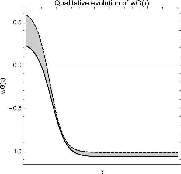
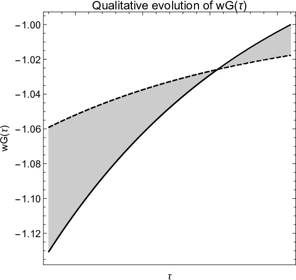
Before we proceed to our analysis with the case in which we include matter source, in Fig. 2 we present the qualitative evolution of the parameter for the equation of state $w_{G}\left(\tau\right)$, for positive and negative values of the parameter $\mu$ and for $\lambda_{0}=2.$ For positive values of $\mu$, the initial condition is for $x\left(0\right)\simeq 1$, while we observe that the final attractor describes an accelerated universe close to the de Sitter point. On the other hand, for negative values of $\mu,$ i.e. $x<0$ and initial condition $x\left(0\right)\simeq-0.01$, the final attractor is again close to the de Sitter universe. The value of the parameter $\mu$ is unknown, and Fig. 2 provides a qualitative evolution of the equation of state parameter. From the numerical simulation, we observe that the equation of state parameter can cross the phantom divine line which does not contradict the observations [5].

For the power-law potential $V_{a}\left(G\right)$, where $\lambda=const$., i.e. $\lambda=\lambda_{0}$, the dynamical (16), (17) admits the critical points of the form $A=\left(x\left(A\right),y\left(A\right)\right),$

We observe that points $A_{1},~A_{2}$ and $A_{3}$ have the coordinates of $P_{1},~P_{2}$ and $P_{3}$ respectively, while the new critical points are the $A_{0},~A_{4}$ and $A_{5}$. More specifically for each critical point we have:

• •

  Point $A_{0}$ corresponds to the matter dominated era where $\Omega_{m}\left(A_{0}\right)=1$,$~\Omega_{G}\left(A_{0}\right)=0$ and $w_{tot}=0.$ One of the eigenvalues of the linearized system close to the critical point is positive which means that the point is unstable.

• •

  At the point $A_{1}$ the potential $V\left(G\right)$ dominates the universe while $\dot{G}=0$, that is $\Omega_{m}\left(A_{1}\right)=0$ and $\Omega_{G}\left(A_{1}\right)=1$, while $w_{tot}\left(A_{1}\right)=w_{G}\left(A_{1}\right)=-1$. The stability of the point is explicitly that which is described for the point $P_{1}$.

• •

  The discussion of the physical properties for point $A_{2}$ is exactly that for point $P_{2}$, because $\Omega_{m}\left(A_{2}\right)=0$ and $\Omega_{G}\left(A_{2}\right)=1.$ However, the eigenvalues are calculated to be $e_{1}\left(A_{2}\right)=3+\sqrt{\frac{6}{\mu}},$ and $e_{2}\left(A_{2}\right)=6+\left(1-\lambda_{0}\right)\sqrt{\frac{6}{\mu}}$, that is, the point is always unstable because $\operatorname{Re}\left(e_{1}\left(A_{2}\right)\right)>0$.

• •

  Point $A_{3}$ exists for all the values $\lambda$ and $\mu,$ while the physical solution is that described by point $P_{3}$. The eigenvalues of the point are calculated to be $e_{1}\left(A_{3}\right)=-3+\frac{\left(1-\lambda_{0}\right)^{2}}{2\mu}$, and $e_{2}\left(A_{3}\right)=-3-\frac{\left(1-\lambda_{0}\right)\lambda_{0}}{\mu}$. The stability of the point depends on the values of the parameters $\lambda_{0},~\mu~$and specifically the eigenvalues are positive, that is, $A_{3}$ is unstable when (a) $\lambda_{0}\leq-1~$or $\lambda_{0}>1~$and $0<\mu<\frac{\left(1-\lambda_{0}\right)^{2}}{6}$; (b) $-1<\lambda_{0}<0$ and $0<\mu<\frac{\lambda_{0}\left(\lambda_{0}-1\right)}{3}$.

• •

  Point $A_{4}$ describes a universe where $\Omega_{m}\left(A_{4}\right)=1-\frac{2}{3\mu}$ and $\Omega_{G}\left(A_{4}\right)=\frac{2}{3\mu}$; while for the parameters of the equation of state $w_{tot}\left(A_{4}\right)=-\frac{2}{3\mu}$ and $w_{G}\left(A_{4}\right)=-1~$follows. Hence, field $G$ behaves like a cosmological constant and, specifically, that point corresponds to the $\Lambda$CDM cosmology, where parameter $\mu$ is related to the energy density of the dark energy. It is important to mention that the point exists only for values of $\mu$ where $0\leq\Omega_{m}\left(A_{4}\right)\leq 1$, that is, $\mu\geq\frac{2}{3}$. The corresponding eigenvalues of the linearized system are $e_{1}\left(A_{4}\right)=-\frac{9}{2}+\frac{7}{\mu}$, $e_{2}\left(A_{4}\right)=-3+\frac{2\left(2-\lambda_{0}\right)}{\mu};$ thus, we conclude that point $A_{4}$ is stable for $\lambda>\frac{13}{3}$ and $\frac{14}{9}<\mu<\frac{2\left(\lambda_{0}-2\right)}{3}$. However, when point $A_{4}$ is stable, we calculate $\Omega_{m}\left(A_{4}\right)>\frac{4}{7}$, which is bigger value from the observable one, i.e. $\Omega_{m0}\simeq 0.28$. Therefore, in order for the model to be cosmologically viable, point $A_{4}$ has to be unstable.

• •

  Point $A_{5}$ exists when (a) $\lambda_{0}<0$ with $-\frac{\lambda_{0}}{3}<\mu<\frac{\lambda_{0}\left(\lambda_{0}-1\right)}{3}$; (b)$~\lambda_{0}>0$ with $-\frac{\lambda_{0}}{3}<\mu<\frac{\lambda_{0}\left(\lambda_{0}-1\right)}{3},$these ranges are given in Fig. 3. Point $A_{5}$ describes a universe where $\Omega_{m}\left(A_{5}\right)=1+\frac{1}{\lambda_{0}}\left(\frac{3\mu}{\lambda_{0}}-1\right)$; and $\Omega_{G}\left(A_{5}\right)=\frac{1}{\lambda_{0}}\left(\frac{3\mu}{\lambda_{0}}-1\right)$ with equation of state parameters $w_{G}\left(A_{5}\right)=-\frac{3\lambda_{0}}{3\mu+\lambda_{0}}$ and $w_{tot}\left(A_{5}\right)=-\frac{3}{\lambda_{0}}$, where $w_{tot}\left(A_{5}\right)<-\frac{1}{3}$ for $0<\lambda_{0}<9$. The point describes a universe with radiation and dark matter when $\mu=-\frac{10\lambda_{0}}{3}$ and $\lambda_{0}\leq 9$. It is an interesting point because it can describe a phase where radiation dominates the universe for $\lambda\rightarrow 9^{+}$. Point $A_{5}$ is stable when (i) $\lambda_{0}<-1$ with $-\frac{2\lambda_{0}}{3}<\mu<\frac{\lambda_{0}\left(\lambda_{0}-1\right)}{3}$ and (ii) $\lambda_{0}>1$, $0<\mu<\frac{\lambda_{0}\left(\lambda_{0}-1\right)}{3}$ as they are given in Fig. 3.

We continue our analysis with the scenario of the exponential potential $V_{\left(b\right)}\left(G\right)$.

Consider now the exponential potential $V_{\left(b\right)}\left(G\right)$. The dynamical system (16)-(18) has dimension three and the critical points are of the form$~B=B\left(x\left(B\right),y\left(B\right),\lambda\left(B\right)\right)$, in particular

Points $B_{0}-B_{5}$ are specifically points $A_{0}-A_{5}$ respectively, while $B_{6}$ and $B_{7}$ are related to $Q_{4}$ and $Q_{5}$ in the vacuum scenario, and $B_{8}$ is the only new point which is a special of point $A_{4}$ with $\lambda$ zero. Because of that correspondence, it is not necessary to discuss the physical properties of the points; therefore, we continue with the discussion of the stability conditions.

• •

  Point $B_{0}$ is always unstable because one of the eigenvalues is always positive.

• •

  Point $B_{1}$ has two zero eigenvalues, hence central manifold theorem has to be applied. In particular, the coordinates of $B_{1}$ describe a line in the space $\left\{x,y,\lambda\right\}$. We find that the stability and instability of the solution corresponds explicitly to the conditions given by point $P_{1}.$

• •

  Point $B_{2}$ has the eigenvalues $e_{1}\left(B_{2}\right)=3+\sqrt{\frac{6}{\mu}},~e_{2}\left(B_{2}\right)=3+\sqrt{\frac{6}{\mu}}\left(1-\lambda\right)$ and $e_{3}\left(B_{3}\right)=\sqrt{\frac{6}{\mu}}$; hence the point is always unstable.

• •

  Point $B_{3}$ is found to be stable when parameters $\lambda_{0}$ and $\mu$ are given by the following set of ranges: (a) For $\lambda\leq-1$, $\mu>\frac{\lambda_{0}\left(\lambda_{0}-1\right)}{3}$; (b) for $-1<\lambda_{0}<1,~\mu>\frac{\left(1-\lambda_{0}\right)^{2}}{6},$ and (c) for $\lambda>1,$ $\mu<0.$ The surface in the space of variables $\left\{\lambda_{0},\mu\right\}$ in which point $B_{3}$ is stable is presented in Fig. 4.

  

  

• •

  At the point $B_{4},$ the eigenvalues of the linearized system have the simple expressions, $e_{1}\left(B_{4}\right)=\frac{2}{\mu},~e_{2}\left(B_{4}\right)=-\frac{9}{2}+\frac{7}{\mu}$ and $e_{3}\left(B_{4}\right)=3+\frac{2\left(2-\lambda_{0}\right)}{\mu}$, which means that the point is stable when $\lambda_{0}<0$ and $2\lambda_{0}-4<3\mu<0$.

• •

  Point $B_{5}$ is stable when (a) $\lambda_{0}<-1$ and $\mu<0$ or $-\frac{2\lambda_{0}}{3}\mu<\frac{\lambda_{0}\left(\lambda_{0}-1\right)}{3}$ as it is presented in Fig. 4.

• •

  Point $B_{6}$ provides the eigenvalues $e_{1}\left(B_{6}\right)=-\sqrt{\frac{6}{\mu}},~$ $e_{2}\left(B_{6}\right)=3+\sqrt{\frac{6}{\mu}}$ and $e_{3}=6+\sqrt{\frac{6}{\mu}}$ which means that the solution at the point is always unstable.

• •

  Close to point $B_{7}$ the eigenvalues of the linearized system are $e_{1}\left(B_{7}\right)=-\frac{1}{\mu},~e_{2}\left(B_{7}\right)=-6+\frac{7}{2\mu}$ and $e_{3}\left(B_{7}\right)=-3+\frac{2}{3\mu}$, from where it follows that the point is always stable for every value of $\mu>\frac{2}{3}$.

• •

  The eigenvalues at point $B_{8}$ are derived to be $e_{1}\left(B_{8}\right)=-\frac{2}{\mu},~e_{2}\left(B_{8}\right)=3+\frac{4}{\mu}$ and $e_{3}\left(B_{8}\right)=-\frac{9}{2}+\frac{7}{\mu},$ which means that the point is always unstable.

It is important to mention that our study for the power-law and the exponential potentials coverS all the possible physical states which can be determined by the dynamical system (16)-(18). The only differences will be on the stability of the points. Therefore, it is not necessary to extend the present analysis for other kind of potentials.

In order to explain the latter statement, we not that any stationary point corresponds to a value $\lambda_{0}$ such that $\Gamma\left(\lambda_{0}\right)=const.$ Now we can always rescale a new variable $\bar{\lambda}_{0}$, such that these points to be described by the exponential potential. For instance, consider the hyperbolic potential for the minimally coupled scalar field studied in [77, 78, 79]. The admitted critical points [80] correspond to eras where the hyperbolic potential mimics the exponential potential or the power-law potential [81].