Progress and perspectives on composite laser-pulses spectroscopy
for high-accuracy optical clocks.
Abstract
Probing an atomic resonance without disturbing it is an ubiquitous issue in physics. This problem is critical in high-accuracy spectroscopy or for the next generation of atomic optical clocks. Ultra-high resolution frequency metrology requires sophisticated interrogation schemes and robust protocols handling pulse length errors and residual frequency detuning offsets . This review reports recent progress and perspective in such schemes, using sequences of composite laser-pulses tailored in pulse duration, frequency and phase, inspired by NMR techniques and quantum information processing. After a short presentation of Rabi technique and NMR-like composite pulses allowing efficient compensation of electromagnetic field perturbations to achieve robust population transfers, composite laser-pulses are investigated within Ramsey’s method of separated oscillating fields in order to generate non-linear compensation of probe-induced frequency shifts. Laser-pulses protocols such as Hyper-Ramsey (HR), Modified Hyper-Ramsey (MHR), Generalized Hyper-Ramsey (GHR) and hybrid schemes are reviewed. These techniques provide excellent protection against both probe induced light-shift perturbations and laser intensity variations. More sophisticated schemes generating synthetic frequency-shifts are presented. They allow to reduce or completely eliminate imperfect correction of probe-induced frequency-shifts even in presence of decoherence due to the laser line-width. Finally, two universal protocols are presented which provide complete elimination of probe-induced frequency shifts in the general case where both decoherence and relaxation dissipation effects are present by using exact analytic expressions for phase-shifts and the clock frequency detuning. These techniques might be applied to atomic, molecular and nuclear frequency metrology, mass spectrometry as well as precision spectroscopy.
I Introduction
The history of very high precision spectroscopy started in the 1930s with the atomic and molecular beam resonance method proposed by I.I. Rabi to improve the resolution of nuclear moment measurements [1]. The original experiment was based on a combination of inhomogeneous fields and a rotating field to flip nuclear spins and measure the magnetic moment of the species. With enough interaction time and under a quasi-resonant irradiation, coherent oscillations can be achieved between targeted quantum states which are manipulated by an external coherent field with tunable amplitude and frequency. In such a case, the final two-level occupation probabilities can be controlled with an adequate selection of a radio-frequency field and pulse duration. By scanning the frequency of the electromagnetic excitation around the exact resonance, a narrow spectroscopic transition is observed which can be used to obtain a very narrow discriminator, stabilizing the frequency of a local oscillator on the atomic frequency for instance, thus achieving an atomic clock. The Rabi technique provided plenty of information not only on atomic and molecular structure, but also on nuclear properties [2].
To improve the frequency resolution, Ramsey designed a scheme, where he replaced the single oscillatory field by a double microwave excitation pulse separated by a free evolution time [3]. The probing electromagnetic field perturbation on the atomic transition itself was reduced by averaging the probe induced frequency-shift over the entire sequence of pulses separated in space or time [4]. Such a technique has drastically impacted time and frequency metrology with microwave atomic clocks since the 1950s [5, 6, 7]. This protocol also provides the highest resolution for evaluation and reduction of systematic frequency shifts perturbing an atomic transition.
Atomic optical clocks are today recognized to be ideal platforms for highly accurate frequency measurements, leading to very stringent tests for physical theories and variations of the fundamental constants with time, and also for quantum simulation investigations, as reviewed in [8]. Depending on the selected atomic species used to achieve stable and accurate optical frequency standards, single trapped ion clocks [9, 10, 11] and neutral atoms lattice clocks [12, 13, 14] have been characterized over many years, reducing systematic uncertainties to a value surpassing current microwave atomic frequency standards. Very long storage time of Doppler and recoil-free quantum particles have been obtained using laser cooling techniques and a relative accuracy level below will most likely be achieved in the near future. This uncertainty reduction will be obtained thanks to a combination of technological advances, but also to the development of ad-hoc protocols.
The present work reports the recent advances on the development of those protocols, where the interrogation process is composed by a sequence of laser pulse. The basic idea is to drive the quantum system by a sequence of pulses whose composite action produces the planned target state. A tuning of the pulse parameters leads to the compensation of the quantum imperfections. Few composite pulse schemes were inspired by nuclear magnetic resonance (NMR) [15] and quantum information processing [16, 17]. As tested in the experiments of refs. [18, 19, 20, 21, 22], this approach improves the performance of optical clocks based on ultra-narrow atomic transitions, by relaxing the sensitivity to clock interrogation disturbances.
Even if a clock optical transition has a very narrow linewidth, the clock interrogation process may limit the final accuracy. The limitations have different sources as the laser probe frequency/intensity instabilities, light-shifts associated to the very weak excitation of additional optical levels of the atom/ion, decoherence and relaxation of the probed atomic system. In weakly allowed transitions with fermionic species, the frequency light-shift is usually small and does not represent an important contribution at the relative level of accuracy presently reached [23, 24]. However, for clocks operating on strongly forbidden transitions and very long natural lifetimes, or for clocks using less stable local oscillators, shorter and more intense pulses are a necessity and may generate an important light-shift of the clock transition. These light-shifts represent a non-negligible issue for clocks either based on a single trapped ion, or on bosonic neutral atoms with forbidden dipole transitions activated by mixing a static magnetic field with a single laser [25, 26], magic-wave induced transition in even isotopes [27], or an E1-M1 two-photon laser excitation [28, 29, 30]. In order to eliminate those systematic frequency-shift induced by the probe laser below the accuracy level, it is necessary to develop new and very robust spectroscopic techniques schemes.
This elimination of systematic frequency shifts based on new spectroscopic techniques is characterized by an important historical evolution. In NMR, the key issue is to tackle systematic effects responsible for imperfect rotations of the nuclear spins, because of the use of a non uniform electromagnetic field for instance [15]. Composite rotations manipulating the quantum system have been extensively developed to get rid of dual imperfections from pulse length error and resonant offset detuning. The composite pulse approach has been also applied in quantum computation to correct imperfect operations on qubits. It was theoretically investigated for a scalable quantum computer, based on trapped electrons in vacuum, where qubits are encoded in the external (cyclotron motion) and internal (spin) degrees of freedom [31]. This approach allowed manipulation of the cyclotron motion without modifying the spin evolution. In [32] several sequences of NMR-type composite pulses were applied to manipulate a thermal cold atom cloud for interferometric applications. In [33] composite pulse sequences have been applied to laser and microwave excitation of trapped ions to produce entanglement. In ref. [34] the Ramsey interrogation of ytterbium trapped ions was modified by adding a central off-resonant approximate pulse, in a way reminiscent of the spin-echo technique. Playing with the relative detuning between applied pulses, this composite-like method eliminated small-to-moderate fluctuations in detuning, thereby greatly enhancing the fringe contrast in the presence of laser detuning drifts.
The optical-clock protocols are the results of a theoretical effort of deriving ad-hoc time-dependent Hamiltonians compensating the clock limitations listed above. Historically the first clock synthetic Hamiltonian is the well-known Ramsey protocol with separate oscillating fields creating an interference pattern in the clock spectral response. Within the last few year, some new protocols were derived in order to bypass the limitations previously listed and also to match the potential high accuracy of the optical clock new generation. In analogy with NMR techniques presented above, a composite pulse Ramsey (R) spectroscopy, denoted as hyper-Ramsey spectroscopy (HR), modified hyper-Ramsey spectroscopy (MHR) or generalized hyper-Ramsey (GHR) including laser phase steps have been introduced in frequency metrology in order to provide highly efficient correction of the clock light-shift induced by the probing laser [19, 35, 36, 37, 22]. Additional perturbations associated with decoherence due to finite laser spectral width and atomic relaxation by spontaneous emission are also corrected by composite pulses, and in particular by those based on a phase-step during the pulse sequence [38].
This effort may be considered as a rewriting of composite pulses for optical clocks. However the goal is quite different: a resolution increase for NMR, a better accuracy for clocks. This difference implies an accurate control of state populations in the first case. The second case instead requires a precise determination of the free evolution of the quantum system. Therefore the basic tools are similar, but the final protocols different. Let’s also point out the strong similarity between the design of time-dependent Hamiltonians for optical clocks and the realization of artificial magnetism for ultra-cold neutral atoms, as reviewed in [39]. In this case the atomic center-of-mass is controlled by applying an Hamiltonian with proper space-dependence, and the successive application of different Hamiltonian may improve the target of reaching a specific final state. For the optical-clock case, different time-dependent Hamiltonians are applied within a sequence designed for a very accurate measure of the quantum state under exploration. The sequence target is to improve the accuracy and robustness of the measurement itself.
A complementary approach, denoted as synthetic protocol, is based on independent and parallel measurements of several clock-frequency shifts for different free evolution times and an appropriate combination of those measurements to generate the so-called synthetic frequency-shift, that produces the optical clock frequency with a high immunity to the laser probe perturbations. This approach, presenting large advantages in presence of an atomic decoherence, may be considered as a different composite pulse protocol, where a different parameter of the Ramsey’s interrogation scheme is properly varied: the free evolution time. The a posteriori treatment of the independent measurements applied within the synthetic protocol constitutes also an element of the phase-step protocols.
Let’s mention here few original features of the composite pulse strategy for the optical clocks. As key point in the determination of the clock proper frequency by eliminating all the shifts produced by different source, the resonant frequency of an isolated atomic or molecular transition is a symmetry point (isolated meaning without a perturbation produced by the presence of a neighbouring transition). That symmetry is associated to the unperturbed atomic response and this symmetry feature characterizes the Ramsey’s free evolution time within the pulse sequence. While the laser excitation and interrogation parts of the composite pulse sequence excite the atoms with different parameters (frequency, phase, and so on), the probe signal produces an atomic response ”averaged” over all the pulse sequence. The central symmetry point should appear in that response: the composite pulse protocol reaches this target applying properly chosen parameters.
In most atomic frequency standards, the laser probe is stabilized to the atomic transition by a frequency modulation technique. Probe-induced shifts introduce a distortion of the absorption line-shape and modify the clock operating frequency. In order to eliminate the asymmetry effect on the true clock position, a phase-step modulation was proposed and tested in [40, 41, 42, 43, 44]. The phase-step composite pulse protocol introduces a similar but more sophisticated approach: the error signal is given by the difference between two different transition probabilities in presence of phase steps within the composite pulse sequence. Here a technical feature introduced in order to improve the signal quality is translated into the construction of ad-hoc Hamiltonians.
Even if the probe laser is pre-stabilized on a high-finesse Fabry-Perot cavity, the resulting finite line-width of the laser is often limited by thermal noise [45, 46]. For the clock atoms this limiting line-width represents a dephasing process which deteriorates the clock interrogation, reduces the contrast and compromises the robustness of any error signal. Fast improvements in the design of very high finesse Fabry-Perot cavities used to stabilize clock lasers should offer in the future very narrow line-widths below a few 100 mHz [47, 48, 49] for a new generation of frequency standards. Actually, this decoherence issue has been treated within the contest of the composite pulse protocols. Let’s point out that the decoherence produced by the laser line-width dephasing does not influence the free evolution time, that represents the most important element in the precise recovery of the clock transition frequency. Instead it influences the atomic evolution within the excitation periods. The operation of most composite protocols is heavily compromised by the decoherence presence. However the construction of ad-hoc Hamiltonian protocols produces a very large reduction of its role, greatly compensating the laser probe shifts and the dependence on the laser excitation parameters, i.e., intensity and interaction time. This is an important result because decoherence are usually considered as a strong limit on the reachable accuracy, and because the decoherence role is circumvent by Hamiltonian interactions. This result is a part of the present large interest into the control over dissipative processes and to the realization that the coupling to the environment can be manipulated to drive the system into desired quantum states [50, 51].

This work reviews the theoretical and experimental efforts performed so far on the optical clock composite pulse schemes for a robust compensation of features such as light-shifts, laser probe frequency and intensity induced instabilities, decoherence and relaxation. Section II, after introducing the wave-function formalism for a two-level atomic system in coherent interaction with a laser, investigates the NMR-like composite pulses and their simplest R and HR composite pulse counterparts. The benefits and limits of the R and HR schemes are presented. Section III emphasizes the laser phase manipulation of each individual pulse through laser steps as a key parameter to improve clock operations. Probing schemes like HR, MHR, GHR containing phase-steps are described. Section IV presents optical Bloch-equations describing coherent interaction between laser and atoms, including several dissipative processes disrupting clock operation. It is shown how the combination of GHR error signals can provide immunity to both decoherence and relaxation. Section V discusses the synthetic frequency approach. A recent experimental modification of the Ramsey configuration, denoted as auto-balanced Ramsey spectroscopy, is also briefly discussed. Section VI reports two recent experimental implementations based on HR and MHR composite laser-pulses protocols on a single 171Yb+ ion [20] and on 88Sr bosonic atoms optically trapped at a magic wavelength [22], respectively. Conclusions and perspectives terminate our review.
II Ramsey and Hyper-Ramsey interrogation schemes
A frequency standard, shown in Fig. 1, requires locking and stabilizing the phase or the frequency of an external oscillator to some atomic or ionic transition by means of laser spectroscopy. Higher frequencies and ultra-narrow lines improve measurement precision. This is the reason why the field of frequency metrology has moved over several decades from microwave transitions to optical narrow lines [8]. Weakly allowed or forbidden clock transitions are now widely investigated for the next generation of high-accuracy frequency standards based on a single trapped ion [10] and neutral atoms in optical lattices [52, 12, 13]. Depending on the nature of the quantum absorbers, i.e fermionic or bosonic particles [53], using either a single stabilized clock laser [27], a combination of static magnetic field and laser [25, 26, 54, 55] or several oscillating laser fields may be exploited to probe the atomic transition [28, 29, 30]. In the following we consider a two-level system interacting with a single EM field without loss of generality.
A Doppler recoil-free atomic clock as depicted in Fig. 2 can be implemented as a two-level quantum system with energy splitting . We start with a typical description of coherent atom-light interaction where external perturbations like decoherence, collisions between particles and all atomic level relaxations are neglected. The two-level system is probed by a clock laser at frequency . Within rotating wave approximation (RWA), the interaction is governed by the complex Rabi frequency including the laser phase , where the th subscript will denote the number of the applied laser pulse in an interrogation pulse sequence. The clock laser detuning from the unperturbed transition frequency is:
| (1) |
A two-level system is a good approximation for most spectroscopic investigations, but is not suitable for high-resolution spectroscopy in the case of optical clocks. With a two-level transition, the virtual excitation of external non-resonant states leads to light shifts of energy levels [56]. We define as the probe-induced frequency shift altering atomic energies while the probe laser is switched on. It is proportional to the laser probe intensity. It can sometimes be useful to compensate for that light shift by stepping the laser frequency during pulses by a fixed amount . Therefore we introduced as the effective total detuning:
| (2) |
The above equation introduces the residual uncompensated frequency shift as the difference between the external laser probe-induced frequency shift and the laser frequency step used to cancel it (see Fig. 2). Because the and are very small compared to the detuning of the non-resonant states, is constant over the whole clock interrogation process if the probe laser intensity is constant.

It is important here to stress the operational difference between a laser spectroscopy experiment and an optical (or microwave) clock. In a spectroscopic investigation, the frequency is controlled independently from the atom (or sample) to be explored. Within a clock, a servo-loop system is applied as depicted in the upper left of Fig. 1 producing the probe laser oscillation at clock frequency . The purpose of the servo-loop system, including the composite pulse interrogation, is to compensate light shifts and produce , that is a zero offset . An imperfect (or real!) clock operates with an arbitrary small offset, or equivalently the atoms are probed by a laser which misses resonance, that is . In the following we investigate several protocols aiming to cancel even in presence of a probe-induced shift correction different from zero.
II.1 Single or adjacent pulses: Rabi interrogation and NMR-like composite pulses for robust population transfer


The superposition of clock states induced by a laser (or RF) pulse is described by the following linear combination:
| (3) |
where and are probability amplitudes related to states and respectively. The parameter is here defined as the effective pulse area :
| (4) |
with being the laser pulse duration and where we introduce a generalized Rabi frequency for convenience. If the total atom-laser interaction time is shorter than the damping times for the dissipation mechanisms discussed in Sec. IV, clock state dynamics are described by the following set of Schrödinger’s equations:
| (5) |
Using the solution of Schrödinger’s equation, the matrix solution for transition amplitudes can be written as:
| (6) |
including a phase factor of the form . The wave-function evolution driven by a pulse area is determined by a complex interaction matrix as [57, 58, 59]:
| (7) |
Applying the above matrix with initial conditions , a final complex amplitude is obtained, leading to the well-known Rabi transition probability :
| (8) |
In Rabi’s original experiment [1, 2], a thermal molecular beam passes through a coil excited by a radio frequency (RF) field with interaction time . The time of interaction and the field amplitude are chosen such that the product , a so-called pulse, corresponds to a pulse area. If the radio frequency is tuned to the transition, at time all particles with are detected in their excited state. In this configuration, the single field has to be perfectly controlled and homogeneous in the interrogation zone to achieve good sensitivity. Fig. 3a shows the Rabi spectrum associated with the single pulse excitation scheme obtained by scanning the frequency detuning. As shown by the Fourier transforms of Fig. 3a, the Rabi line-shape exhibits a decreasing width with increasing excitation time. The resolution of this spectroscopy is limited by the flight time of particles through the coil. The FWHM width of a pulse is (in Hz). An increase of the duration is possible to a certain extent, but for experimental reasons, it becomes difficult to maintain the appropriate microwave field for long periods or large pulse areas. It is important to note that in this case, the clock frequency-shift of the transition probability is always linearly dependent on the residual uncompensated part of the light-shift. In modern optical ion and lattice clocks, the Rabi spectroscopy has been mostly implemented to obtain very high resolution measurements of various metrological clock transitions with low systematics [8].
| Pulses area | ||
|---|---|---|
| low | low | |
| low | medium | |
| medium | low |
If several adjacent pulses are used, the single matrix of Eq. (6) is replaced by a product of several matrices in order to explore various sequences based on NMR-like composite pulse excitations. Tab. 1 reports examples of Rabi composite pulses inducing a robust population transfer between two targeted quantum states required either for offset detuning or RF field compensation [60]. The Table first column introduces a compact indication of the composite pulse composition. The lineshapes for different NMR-like composite pulses are shown in Fig. 3b and Fig. 3c. The corresponding contour plots in the right column of Fig. 3 evidence the optimized robustness of the population inversion by using several adjacent pulses optimized against uncompensated residual frequency-shifts in Fig. 3b, and against important pulse area variations in Fig. 3c.
II.2 Pulses with an interleaved free evolution time: Ramsey and Hyper-Ramsey schemes

Within the original R spectroscopy configuration, atoms are probed by two successive pulses separated by a free evolution time T [3]. During free evolution time T where the probe laser is switched-off, the matrix given by Eq. (7) does not contain the light-shift from external off-resonant states. The free-evolution transfer matrix reduces to:
| (9) |
because no additional laser frequency step is applied during free evolution time.
In the HR interrogation three pulses are applied, with a free evolution time after the first or second pulse [19], see an example in Fig. 4 with the free evolution time applied after the first pulse. Note that another composite sequence with pulse order reversal can be also used as proposed in [35]. The coherent population transfer induced by such pulse sequences is given by a simple product of matrices, each of them being individually tailored in frequency, duration and phase. If pulses are labeled by , the corresponding transition probability is given by:
| (10) |
where we introduce . The composite pulse sequence may
includes a laser phase-step during each pulse which can be manipulated to control the resonance shape. This applies to the HR- protocol of Fig. 4 where the pulse sequence includes a laser phase sign inversion during the second interaction. The transition probability describing the coherent population transfer between atomic states depends on pulse areas and phase jumps over the entire laser probing sequence. By scanning the detuning between the laser and the two-level resonant frequency, a HR resonance
is constructed containing information about perturbations induced by the laser probe on the line-shape.
Ignoring for simplicity the additional phase step, the expression can be written in a compact form as:
| (11) |
where is the clock frequency detuning during free evolution time. The envelopes are given by
| (12) |
and the phase
| (13) |
The envelopes , and the phase driving the resonance amplitude are given in Appendix VII.1. This formula is valid only for phase jumps within the pulse sequence. However note that the general form valid for arbitrary phase steps, described in the following by Eq. (28), has the same structure of the above one. Using Eq. (11), and its generalization in presence of phase-steps derived in ref. [35], the population transfer efficiency and the frequency-shift affecting the resonance can both be evaluated accurately under various experimental laser pulse conditions including R and HR schemes [3, 19].
When the second pulse area vanishes, i.e , i.e. , and , , , the generalized transition probability takes the following form:
| (14) |
with in Eq.(11), and for the phase
| (15) |
By applying a trigonometrical transformation, we recover the standard expression for the transition probability derived by Ramsey in 1950 for a spin interacting with a radio-frequency field [3, 4] as:
| (16) |
This expression established by Ramsey [3] was the initial version of the method of separated oscillating fields in molecular beams.
A remarkable information is the frequency-shift generated by Eq. (14) that determines the central fringe position sensitivity to a detuning fluctuation. From a geometrical point of view, this Ramsey phase-shift is exactly two times the Euler angle accumulated by a Bloch’s vector projection of rotating components in the complex plane using a two dimensional Cauley-Klein representation of the spin 1/2 rotational group [57].
The separated oscillating fields method invented by Ramsey and presented in Fig. 5a
effectively reduces the clock sensitivity to light-shift effects. Interference fringes in the population transfer, as shown in
Fig. 5a, are observed versus the clock laser detuning and the central feature is used to lock
the local oscillator to the atomic or molecular transition. It has been widely applied in high precision measurements for atomic clocks
based on atomic beams crossing a microwave cavity twice [7, 6, 5] and was extended to Zacharias-type
fountain geometries where laser cooled atoms are thrown up vertically [61, 62]. In the last device, a cold
atomic cloud experiences a first pulse () during its rise when passing through a microwave
resonator, then freely evolves without light interaction during its free launch and free fall. Finally it undergoes a second
pulse in the same cavity before detection.
The resolution of such a clock configuration is only limited by the atomic cloud time of flight T between microwave interactions
[63]. The resonance width (in Hz) is when . The reduction of the Ramsey clock frequency-shift
reported in Fig. 5a by the factor was observed in molecular beam experiments
with RF fields [64, 65, 66, 67].
Despite its great resolution, the original Ramsey method remains
too sensitive to perturbations from the optical probe laser field itself. Some spatial laser beam configurations where proposed
in the 1980’s by Bordé canceling first-order Doppler-shifts to observe optical Ramsey fringes [68].
However, if external AC Stark-shifts are not reduced or potentially eliminated, the Ramsey central fringe is pulled away from resonance and the fringes themselves become asymmetric around the
maximum [69]. This asymmetry was observed for single ion clock using an ultra-narrow electric electric octupole (E3)
optical transition [10] and in some alkaline-earth neutral bosonic clocks with completely forbidden transitions
[8].


Few techniques were proposed to solve such a problem. A spectroscopic laser probe configuration based on a pulsed EIT (Electromagnetically Induced Transparency)/Raman two-photon excitation suggested in 2006 introduces internal ac Stark-shifts of a three-level system in order to counteract the light-shift contribution from external off-resonant states. This approach restores the Ramsey fringes at the unperturbed clock frequency [29]. A modified Ramsey method was also proposed to cancel the overall light-shift with deliberate application of a laser frequency step during light pulses [18]. However, all these methods require exact knowledge of the light-shift correction or an excellent control of laser power variations to efficiently compensate frequency shifts.
The HR spectroscopy was proposed in 2010 to relax the constraint on laser power control and to eliminate the probe induced frequency-shifts [19]. The scheme is based on pulses that can have different lengths, frequencies, and possibly phase inversion. The initial version is based on a sequence of two different pulses, a first pulse of length as in the Ramsey’s technique, and a second pulse of length , tailored in two parts and . A laser frequency step for a basic pre-compensation of the light-shift is also introduced during pulses to correct the expected external light-shift from off-resonant states of the probed two level system. The transition probability describing the HR resonance, reported in Fig. 5b, has a fringe inversion at the resonance because of the pulse area. A discriminator slope to lock the laser frequency is obtained by a phase modulation on one of the pulses. Even if the phase is discussed in detail within the following SubSection, let’s point out here the presence of a small sensitivity to pulse area variation, limiting the method’s efficiency. This result is shown by the shaded area on the right panel of Fig. 5b. That sensitivity can be compensated by applying a laser phase step during the -length pulse, as in the HR- composite pulse of Fig. 4. Therefore the HR- sequence can be seen as an echo pulse [19]. The important result is a strong non-linear cubic dependence of the central fringe frequency shift with the uncompensated light-shift , see on the right in Fig. 5c. This drastically reduces residual uncompensated light-shift contribution to a very low order.
II.3 Canonical form of the clock frequency-shift
This subsection examines the clock-frequency shift which impacts the Ramsey interference pattern as described by Eq. (11). A good approximation of the shift for the central fringe extremum is given by the following simple relation:
| (17) |
It is thus possible to eliminate the frequency shift of the central fringe by engineering with special choices of laser step frequency, pulse duration, and phase inversion.
A more sophisticated expression for the composite clock-frequency shift than Eq. (17) is needed if the line-shape is perturbed by weak distortions due to decoherence, as derived in Section V.3. The central fringe frequency-shift is thus calculated by applying a first-order expansion to Eq. (11) around the unperturbed frequency clock detuning of the resonance. The result takes the form:
| (18) |
where is the partial derivative with respect to the unperturbed clock detuning . The main term is modified by two high-order phase-shifts as follows:
| (19) |
where
| (20a) | ||||
| (20b) | ||||
The high-order expressions given by Eq. (20a) and Eq. (20b) account for a possible distortion of the line-shape when the free evolution time T is not very large compared to each pulse duration (). This is shown in Fig. 6 for the HR- protocol and various Ramsey free evolution times and a fixed pulse duration.
The analytical expression of the clock frequency-shift for the two-pulse R protocol is written in a simplified expression as [35, 36]:
| (21) |
and in an alternative expression,
| (22) |
to be compared to the following one for the three-pulse scheme.
In the case of three different pulse areas, the HR and HR- phase shifts are derived in [19, 35]. Following [70], they can be rewritten into a closed form solution as:
| (23) |
where the reduced notation of Eq. (57) was inserted within the last term.

For the R, HR and HR- protocols the clock frequency phase-shift based on Eq. (18) is plotted on the right column of Fig. 5 versus the uncompensated residual frequency shift . Here and in following figures they are plotted in the case of during each laser pulse.
In the R case, the clock frequency shift is linearly dependent as shown in
Fig. 5a. As in Fig. 5b for the HR technique based
on the combination and , to be inserted in Eq. (21), the clock becomes non linear. A relative variation of for all pulse
areas affects the protocol and requires a careful control to avoid significant shifts. Fig. 5c presents the clock frequency-shifts of the HR- technique including a laser phase inversion coupled with a pulse. By inserting in Eq. (23) the pulse areas
and while fixing the intermediate laser field phase
to (), a very good compensation of the relative pulse area variation is obtained.
These plots clearly show that composite pulses are really efficient to extend the region where both pulse area variations and residual
light-shifts are simultaneously rejected to a very low level of perturbations. HR spectroscopy is now implemented in single ion clocks
based on ultra-narrow transitions [20, 21], as presented in Section VI.
Fig. 6 shows the comparison between clock frequency shifts computed from Eq. (17),
Eq. (18) and the numerical tracking of the extremum of the central fringes. The high-order corrections given by Eq. (18) are in very good agreement with numerical trackings for all free evolution times. On the contrary, differences exist between
the results based on Eq. (17) analytical expression and those of the numerical tracking, becoming more pronounced when the free evolution time is comparable to the pulse duration.
III Composite Ramsey spectroscopy with phase-step protocols
| protocols | composite pulses | ||
|---|---|---|---|
| R |
| ||
| HR- |
| ||
| MHR |
| ||
| GHR |
| ||
| GHR |
|
In most atomic frequency standards, the laser probe is stabilized to the atomic transition by a standard frequency modulation technique applied at the half-height of the central Ramsey fringe. But if some AC Stark-shifts are present due to non-resonant atomic states, the line-shape is distorted and shifted from the correct clock frequency, leading also to errors and instabilities in the frequency lock point. The proper strategy to eliminate the asymmetry effect on the true position of the central fringe and to generate a robust and stable lock-point for the local laser probe oscillator is the phase-step modulation, as proposed and tested in [40, 41, 44, 43]. In addition this phase modulation technique produces an error signal with enhanced immunity to potential offset variations [41, 42]. A corresponding composite pulse approach is characterized by the presence of appropriate phase-step modulations within specific areas of the pulse sequence. The measured signal is based on a difference of properly chosen generalized transition probabilities following the application of the phase-step modulation. The signal becomes anti-symmetric with respect to the clock laser detuning . This Section presents the composite pulse phase-step protocols of Table 2. Frequency lock points generated from these configurations are well protected against large laser pulse area variations and potential errors in the frequency shift compensations, because they decouple the unperturbed frequency measurement from laser intensity variations [22, 37].


III.1 Transition probabilities including laser phase-steps and error signal definition
Within a GHR sequence, the second or first Ramsey pulse is divided into subsections with individual manipulation of frequency, duration and laser phase, as shown in Fig. 7 for two types of laser pulsed sequences, GHR and GHR. The calculations of different error signals require to explicitly include the laser phase dependence, produced by the phase steps, within the matrix elements in Eq. (7). The GHR transition probability is expressed by:
| (24) |
where the envelopes and of the two sequences are given in Appendix VII.2, taking into account both laser phases and initial atomic preparation. The composite phase-shift represents the atomic phase accumulated by the wave-function during the -th laser interrogation sequence. It is expressed for two different pulse sequences as follows.
For the GHR sequence:
| (25) |
And for the GHR sequence:
| (26) |
in both cases, reduced matrix components are given in Appendix VII.2.
In the case of phase-step protocols, the dispersive-shape of the error signal is computed by taking the difference between two spectroscopic signals with opposite phase and as:
| (27) |
It may be written as
| (28) |
where
| (29a) | ||||
| (29b) | ||||
and
| (30) |
with A and B related to and by Eq. (12).
This laser frequency stabilization scheme synthesizes an anti-symmetric error signal, i.e., a dispersion line-shape, to lock the laser frequency to the center of the unperturbed clock transition. The frequency lock point shift from the error signal due to an imperfect light-shift compensation is directly given by the relation:
| (31) |
Using Eqs. (28) and (31), the analytical form of the frequency-shifted lock-point is
| (32) |
This expression is similar to the rotation parametrization applied in quantum computing to achieve robust cancelations of systematic errors [71, 72].
III.2 Error signals of R and HR schemes
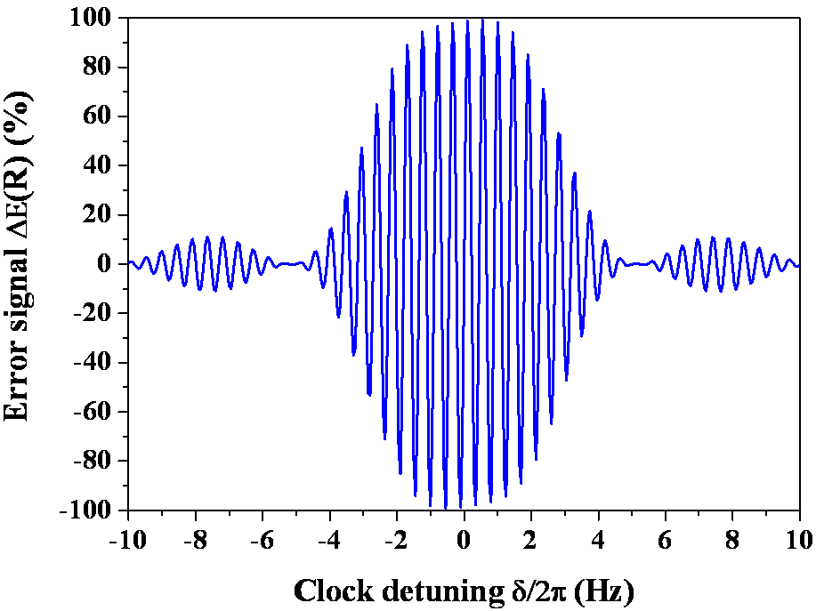
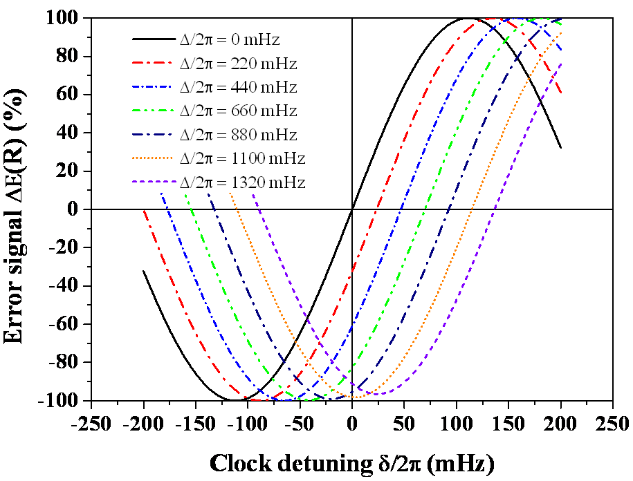


This Subsection, as well the next one, reviews the robustness of different dispersive errors signals to some residual light-shifts and pulse area variations. Some relevant phase-step protocols are reported in Table 2 for application in R spectroscopy [40, 43, 44] and HR spectroscopy [19, 20, 21].
The first laser phase-step configuration based on the R protocol in Tab. 2 was initially proposed in [40]. Following Eq. (27), the error signal is produced by combining two Ramsey transition probabilities in presence of phase shifts
| (33) |
This approach leads to dispersive-like resonance lineshapes with increased sensitivity to detect the clock resonance frequency. This phase-step modulation was applied to single ion clock devices in order to produce better control of the frequency lock point stabilizing the local laser oscillator [43, 44]. The error signal of the R phase-step protocol is plotted on the top left part Fig. 8a. Its associated dispersive signal is plotted for several values of the uncompensated residual light-shift on the top right part.
The error signal of the second phase-step configuration based on the HR- protocol, presented in Fig. 8b, is based on the same phase-steps in presence of an additional phase reversal of the laser field during the intermediate pulse. Following Eq. (27), the error signal is
| (34) |
The main advantage of such a protocol is to generate a frequency lock point which is driven by a cubic non-linear
sensitivity to the uncompensated residual light-shifts leading to a much better control of the frequency discriminant as shown on the right
of Fig. 8b.
The HR phase-step protocol was proposed in [19] and experimentally implemented on a single ion clock in [20] to strongly reduce the residual probe-induced frequency shift by four orders of magnitude. Recently, using this spectroscopic technique [21], the single ion clock achieved a systematic relative uncertainty of probe induced shifts. This protocol still suffers from small residual light-shifts when exploring a wider range of uncompensated frequency offsets. The HR protocol has a residual uncompensated frequency-shift of around 1-2 mHz over a 220 mHz residual offset which may compromise the access to a clock fractional accuracy below .
III.3 Error signals of MHR and GHR schemes


Spectroscopic schemes using different phase-step protocols have been recently introduced in order to completely eliminate residual
light-shift corrections on the central fringe over large uncompensated residual light-shifts.
These are the MHR [22] and GHR [37] schemes.
These new dispersive error signals are centered at the unperturbed atomic resonance with steep discriminants which are impervious
to variations in laser probe induced clock frequency shifts.
The error signals are built from a combination of different transition probabilities as in [22, 37]:
| (35a) | ||||
| (35b) | ||||
The MHR protocol described by Eq. (35a) is based on a superposition of two HR- transition
probabilities. For error signal generation, the phase-step modulation is obtained by interleaving a HR- protocol from
Tab. 2, where during the first pulse, with a HR- protocol
where an opposite phase is used during the last pulse.
The calculated dispersive error signal shape is presented in Fig. 8c along its frequency
lock point response to residual probe-induced shifts.
This non standard protocol was the first to synthesize an error signal yielding full immunity to residual probe light-shifts and great
robustness to pulse area errors originated from laser power variations. It has been successfully tested in a neutral atom optical lattice clock
based on magnetically induced spectroscopy [22] demonstrating suppression of a sizable probe Stark
shift to below even with very large errors in shift compensation.
The GHR() and GHR() protocols from Tab. 2, proposed in
[37] and shown in Fig. 9a and Fig. 9b, respectively, use a single either
or a phase-step modulation during the intermediate pulse.
The associated error signals computed using Eq. (35b) are presented in the same figure. The plots of their
lock point sensitivity shown on the right in Fig. 9a and
Fig. 9b, evidence that they are fully protected from errors in residual probe-induced
light-shifts.
Another stabilization scheme can be generated by combining the error signals of the GHR() and GHR()
protocols, presenting opposite slopes of the error signal. This hybrid scheme denoted GHR() is defined by the
following normalized difference between two error signals:
| (36) |
We have reported the corresponding error signal shape in Fig. 9c. A combination of such protocols will be demonstrated to be efficient in presence of decoherence and relaxation (see V).
III.4 Robustness of error signal slopes
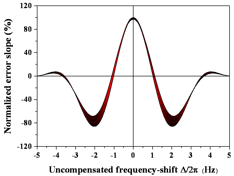


This subsection presents parameters useful to setup optimal working conditions in interrogation
protocols in order to achieve a very efficient lock of the local oscillator to the unperturbed optical clock transition [73].
For simplicity, and because out of scope of this work, we neglect statistical fluctuation in the measured signals produced by external time-dependent perturbation or phase noise contribution [74, 75].
We study the stability and robustness of error signal slopes at against residual uncompensated light-shift
associated to small variations of pulse areas. The frequency stability
scales as the inverse of the slope and a reduced slope results in a clock instability.
Error signal slopes against residual shifts for all protocols are shown in Fig. 10 for a
pulse area variation.
Compared to standard error signals based on R protocol in Fig. 10a and HR protocol in Fig. 10b, the new protocols expand the possible range for the uncompensated shift, i.e., the range between two zero crossings of the error slope.
Both residual uncompensated offsets and pulse area variations are directly transferred to a slope
reduction of error signals with no change in their frequency lock point. However the MHR protocol shown in
Fig. 10c presents a small shape asymmetry and a tiny deviation of the maximum slope value from .
Note that the GHR protocol, shown in Fig. 10f, eliminates unstable operation by an undesired sign inversion of the slope when the uncompensated light shift is too large.
If the light shift is not constant over the pulse sequences, and therefore a large residual offset is present, a strong distortion or rotation of the error signal slope is originated (see for example Fig. 8b, Fig. 8c and Fig. 9) and it may compromise the lock point stability and degrade the clock operating condition. Then, the laser compensation step should be checked and steered to the point where .
Various implementations have been experimentally tested. For the single ion clock frequency standard [20], a stabilization using the HR phase-step protocol scheme was combined with a second interleaved servo system where Rabi spectroscopy with the same probe light intensity is used. Then, the frequency difference between the two interrogation techniques was used to control laser frequency step . This method ensures that slow drifts of the light-shift will not degrade its suppression. It is also possible to use some clock frequency-shift symmetries offered by the MHR protocol with the uncompensated part of the probe shift to design an efficient steering process to [22].
IV Protocols based on free evolution time combinations
This section reviews some combinations of R and HR interrogation protocols with different free evolution times. The target is to generate a clock frequency-shift strongly protected against residual light-shifts over larger offset clock detunings. Some non-linear clock frequency-shifts can be synthesized specifically to be extremely robust against decoherence and relaxation.
IV.1 Synthetic frequency protocol for HR spectroscopy
The synthetic shift technique reduces the sensitivity to pulse area variations and extends the non-linear efficiency of HR protocols to larger uncompensated residual light-shifts. It is based on both independent and parallel measurements of several clock-frequency shifts for different free evolution times and careful combination of those measurements to generate the so-called synthetic frequency-shift. This approach is more robust than previous phase-step locking protocols, reducing both residual uncompensated light-shifts and laser power variations even in presence of decoherence.
The synthetic frequency method, discussed in detail in [38], is based on a polynomial serie expansion of the clock’s residual frequency shift on its dependence to free evolution time T under frequency stabilization:
| (37) |
The coefficients depend on pulse parameters (durations, amplitudes, phases) and uncompensated frequency shift . This method was originally designed to allow suppression of the black-body radiation shift experienced by atomic clocks [76], but it can easily be extended to handle arbitrary systematic shifts (Stark shift, Zeeman shift, and so on).
The basic idea is to build a synthetic frequency using multiple HR sequences with specific choices of free evolution times (but same pulse parameters, assuming we can enforce exact ratios between Ramsey free evolution times) to cancel contributions up to a given order in Eq. (37). For example, using two sequences with free evolution times and , and stabilized frequencies and shifted by and , respectively, the synthetic frequency at the lowest order is defined as
| (38) |
where is the offset detuning ratio. Considering the case of and , it can be shows that the frequency shift can be written as:
| (39) |
Similarly, using three different HR sequences with free evolution times , , and , the shift of the the synthetic frequency at the following order is given by:
| (40) |
Following this pattern to higher orders, it results that the higher orders expansions follow binomial coefficient laws. Using Eq. (56c) for the HR phase shift, the clock frequency shift is calculated on the basis of Eq. (18). Thus, under , the calculations show the following general character of dominating dependencies on :
| (41) |
without synthetic frequency approach, and
| (42) |
for the synthetic frequency approaches at different orders.

Fig. 11 reports the calculations for the above quantities. For the synthetic frequencies, higher-order (more than cubic) non-linearities appear. This character is not changed under variations of , , and T, i.e., we do not need the rigorous condition =. Because in real experiments the value of can be controlled only at the level of 1-10, this method can be very successful in atomic clock implementations.
It is also very important to notice that the combination of the synthetic frequency protocol applied to the HR- scheme is quite stable to decoherence. Indeed, Fig. 12, showing graphs for the above clock shifts against the ratio in the presence of decoherence described by the parameter, demonstrates strong and robust suppression of the shift.

The main advantage of the synthetic method is to reduce the decoherence perturbation without destroying an efficient light-shift compensation using the HR- protocol even when all pulse areas are modified by . The synthetic frequency protocol is also better by one to three orders of magnitude than MHR and GHR() protocols when laser-induced decoherence is considered.
Apart from the combination with Ramsey and hyper-Ramsey spectroscopy for two-level systems, the synthetic frequency protocol can be applied to the Ramsey spectroscopy of coherent population trapping (CPT) resonances (e.g., see [77, 78, 79]). Note that CPT clocks are one of the prospective variants of compact RF clocks with relatively valuable metrological characteristics. Because the probe-induced shift for CPT-Ramsey resonance satisfies the general dependence of Eq. (37) on the free evolution interval T (see [80], where the dependence was found), one can expect good efficiency of the synthetic frequency protocol in this case too. The same approach can also be applied to so-called pulsed optical pumping (POP) clocks [81]. All these examples demonstrate the universality of the synthetic frequency protocol, which can be used in any type of clocks based on Ramsey spectroscopy.
IV.2 Auto-balanced Ramsey spectroscopy
A variant of the synthetic protocol approach, denoted as auto-balanced Ramsey spectroscopy, was very recently presented in ref. [82]. It is based on the combination of two Ramsey sequences, with short and long free evolution times, whence T is the control parameter. The originality of the method is the use of two interconnected control loops. The first feedback loop uses the error signal provided by the short Ramsey sequence to lock an additional phase step correction between the Ramsey pulses, while the second loop locks the mean frequency from the error signal of the long Ramsey sequence. Notice that this sequence contains the phase step correction as an additional control parameter. To demonstrate the efficiency of the auto-balancing approach, the 171Yb+ clock transition was experimentally probed with 3 different technical pulse defects. The auto-balanced Ramsey probing technique was thus able to recover the undisturbed clock transition against pulse areas delivered with 97 of the nominal intensity for the last 3 ms of their 15 ms on-time, against weak phase step excursion of the local laser oscillator and finally against phase lag. A final reduction by about of the light shift was experimentally observed in an 171Yb+ ion clock operating on the E3 transition.
V Composite laser-pulses protocols robust against dissipation
This Section introduces new protocols dealing with the decoherence associated to the finite line-width of the probe laser, which disturbs the clock interrogation by reducing the contrast while also compromising the robustness of any error signal. For the aimed relative accuracy, the decoherence induced by clock laser line-width degrades the robustness of clock lock points for GHR protocols of the last Section. This issue will be mitigated by fast improvements in the design of very high finesse Fabry-Perot cavities used to stabilize clock lasers, thus offering very narrow line-widths below a few 100 mHz [47, 48, 49] for a new generation of frequency standards. However new composite pulse protocols represent an alternative approach to this issue. Relaxation processes for the clock populations are also included into the presented analysis. Notice also that the MHR and GHR() protocols are not fully equivalent in the presence of decoherence produced by the finite laser linewidth [22, 37].
V.1 Matrix solution to optical Bloch equations
The relevant analysis has to be performed within a formalism based on the two-level density matrix where the atomic decoherence can be treated properly [83, 84]. The direct numerical integration of density matrix equations includes dephasing of the off-diagonal elements [85, 86] and relaxation terms of populations, in order to describe dissipative processes such as spontaneous emission, dephasing and decoherence within a closed two-level configuration. The atomic evolution includes a decoherence term , a spontaneous emission rate denoted and a population difference relaxation induced by collisions. The Bloch variables , and are used to describe the atomic excitation after the -th optical pulse of the composite pulse sequence. The general set of time-dependent optical Bloch equations is given by [87]:
| (43) |
The three components vector solution to the previous set of equations is [59, 88]
| (44) |
characterized by the pulse area .
stands for the system’s state before the -th pulse. The steady-state solution matrix
is obtained by
switching off time-dependent derivatives in Eq. (43) for its three components.
See Appendix VII.3 for its definition.
The rotation matrix , taking
decoherence and relaxation terms into account, is written as follows:
| (45) |
requiring the exponentiation of the following matrix:
| (46) |
where we have defined . The matrix can be exactly expressed
as a square matrix of time-dependent matrix elements (), presented in detail in Appendix VII.3.
Consider now a sequence of pulses separated by a free evolution T, as in the HR scheme for example. The free evolution matrix without
laser field is given by
| (47) |
The corresponding stationary solution is also found by switching off the laser field in Eq. (43) during free evolution time.
V.2 Composite interrogation protocol with arbitrary sequence of pulses


When we consider an arbitrary sequence of composite pulses where each laser interaction zone is associated with different areas tailored in phase, frequency and duration, each laser pulse interaction introduced by is described by an equation identical to Eq. (44). An arbitrary sequence of pulses can be constructed by iteration to compute the final response .
Using exact analytic expressions to solve the Bloch equations for a single given Rabi pulse, the expression for a full sequence of n pulses can be generalized to:
| (48) |
where backward arrows indicate a matrix product from right to left with growing indices and state initialization denoted by convention.
Ref. [87] has derived an exact analytic solution for an arbitrary sequence of pulses including a generalized canonical form for the associated phase shift. Such a solution with a single free evolution time can always be expressed in a reduced canonical form as
| (49) |
where the new offset , amplitude and new phase-shift are analytical functions including dissipation explicitly computed in [87]. Notice the equivalence between the present canonical form and those of Eqs. (11) and (28).
Using Eq. (49), we can study the three-pulse interrogation schemes. By looking at the third component , we can retrieve population transitions to construct an error signal. The derived generalized expression for the population of the upper level is formally identical to the transition probability given by Eq. (24) when dissipation is switched-off. The phase-shift including dissipation accumulated over the entire sequence of pulses is now expressed as:
| (50) |
with
| (51) |
and for the components of the product matrix .
| (52) |
The above equations may be used to evaluate the dependencies of clock frequency-shifts to residual light-shifts in presence of decoherence and relaxation processes for any composite pulse protocols, in particular those presented in Tab. 2.
V.3 Elimination of dissipation effects on clock frequency-shift


.
The influence of decoherence or relaxation by spontaneous emission on the HR- probing scheme is analyzed using the 2D contour and density plot diagrams shown on the left in Figs. 13. All clock-frequency shifts , introduced by Eq. (32) in Sec. III for the dispersive clock lock, and determined using the new phase-shift of Eq. (50), are plotted against uncompensated frequency-shifts and large pulse area variations. Because ac Stark-shifts increase quadratically with pulse area, the diagrams explore also regions of several laser pulse area units corresponding to the application of a large laser frequency-step for pre-compensation of the central fringe frequency-shift [18]. Within contour plots, the colored values of clock-frequency shifts have been deliberately limited between -2 mHz and +2 mHz (see layout on graphs) for constraining the clock relative accuracy below . For white surrounding regions, the relative accuracy of the residual shift exceeds a few level. Clock frequency shifts affecting the lock point are reported on the right of Figs. 13. One effect of dissipation is to restore a weak linear dependence to uncompensated residual light-shifts while slope rotation depends on the specific dissipation process.
Fig. 14 reports the clock response to decoherence only for three different protocols. For the MHR protocol, the right plot of Fig. 14a shows a significative frequency-shift at zero residual uncompensated light-shift while its pulse area stability lock point is off axis from . Thus the MHR parasite shift produces a large sensitivity to variations of the Rabi frequency and reduces optimal performances of the stabilization scheme [38]. The GHR() protocols do not suffer from these parasite shifts but the immunity to residual uncompensated shifts is lost when pulse area is not constant as shown in [38]. For the GHR and GHR protocols in Fig. 14b and Fig. 14c, respectively, stability islands exist even when the pulse area is not a perfect .
V.4 Universal interrogation protocols combining and phase-steps


Another stabilization scheme can be generated from the combination of error signals from both GHR() and GHR() protocols, as suggested by the noticeable antisymmetry of their slopes observed on the right side of Fig. 14b and Fig. 14c in presence of decoherence. This hybrid scheme denoted GHR() was defined in Eq. (36). For this protocol, the error signal and its frequency-shift lock-point condition are written, as of Eq. (31):
| (53) |
with the frequency-shift derived from Eq. (32).
In presence of a large residual offset, this scheme reduces the distortion, associated to the GHR() and GHR() protocols. In addition the GHR() protocol leads to a potential suppression of the decoherence effect as proposed in [38]. However it is still sensitive to the presence of relaxation.
A more recent development on composite pulse protocols in ref. [87] has allowed a further improvement of the GHR() protocol. The protocol can be greatly improved by applying it twice while varying the initial state, which is now considered as a parameter to the protocol itself. A new error signal, detailed in Fig. 15a, is built in the following way:
| (54) |
where the index () means the protocol is applied with population initialization in ground state (excited state ), respectively.
This new combination of pulse sequences produces a completely anti-symmetric signal on the population difference Bloch variable W, which directly translates to the transition probability signal. By comparing under identical but now stringent variations of atomic parameters, HR protocol shown in Fig. 16(a) and this protocol shown in Fig. 16(b), it allows for an exact correction of probe-induced frequency shifts in Fig. 16(c) under arbitrarily large light shift effects or laser intensity variations. It yields an exact frequency lock-point of the central fringe while being immune to both decoherence and relaxation. As remarkable feature, this approach is also independent of the initial atomic states as long as they are distinct from each other. This property removes the need for a high precision quantum state initial preparation.
Another approach is to introduce a time reversal of the GHR() protocol. A reciprocal sequence is built by inverting the pulse order in the composite pulse sequence while also inverting all laser phase signs, the so-called GHR†() protocol. It is possible to construct its error signal, detailed in Fig. 15b, as follows:
| (55) |
where stands for the reciprocal sequence’s error signal. This protocol offers the same properties as the previous initial state variation approach with the additional effect of producing an exact anti-symmetric signal for the detection of any Bloch variables. This new feature allows for further detection techniques, for example it is now possible to derive the uncompensated shift from either U or V Bloch variables and predict how the central fringe is shifted from its lock-point before being compensated by applying the error signal. Those last two protocols were introduced and discussed in heavy details in [87].
VI Implementation in quantum metrology
In this last section, we present two different optical clocks based on excitation of a single ion and interrogation of multiple neutral atoms, respectively, which have used composite pulse sequences to eliminate with a very high efficiency the probe induced frequency-shift on clock resonances. Composite pulse sequences have been recently implemented experimentally in the single ion clock developed at PTB (Germany) [20, 21] and in the optical 1D lattice clock with bosonic atoms at NPL (UK) [22]. The single ion clock achieved a reduction of the probe induced frequency-shift by more than four orders of magnitude using the HR protocol [21]. Using a MHR scheme, the optical lattice clock has successfully demonstrated suppression of a sizable probe Stark shift to below even with very large errors in shift compensation [22]. Both clocks benefit from a nearly field free environment and a strong localization of one single particle within an RF trap or several atoms within an optical lattice, allowing for a Doppler-recoil free spectroscopy of ultra-narrow atomic transitions with high accuracy. They are based on very narrow optical transitions, the quadrupole E2 or the octupole E3 transition for the single ion clocks or the forbidden transition in alkaline-earth atomic systems. In both systems, systematic, and problematic, clock-frequency shifts originate from the interaction of the quantum two-level system with the applied laser probe field, and the light-shift produced by off-resonant states not directly addressed by the probe limits the achievable accuracy to the 10-18 relative level.
VI.1 HR protocol with the single trapped 171Yb+ clock
The ytterbium-ion clock transition is unique among optical frequency standards in that the lowest-lying excited state is the state, which decays to the ground state via an electric octupole transition at 467 nm, see Fig. 17. The state is extremely long-lived, with an estimated lifetime of around 6 years. Hence the natural line-width of this transition is of order of the nHz, and is not a limit to the performance of the standard. Instead the stability limit is determined by the probe laser line-width that can be achieved.
The experimental setup is described in Ref. [89, 20]. A single ion is confined in a radio frequency Paul trap. During a first period the ion is successively laser-cooled and pumped to the ground state. The clock transition is then probed by applying an HR sequence, i. e.: time pulse sequence , detuning steps , phase steps . The intensity, detuning and phase of the probe laser beam are precisely shaped by an acousto-optic modulator (AOM). Up to 10 mW of light power can be focused to a beam waist diameter of 40 m at the trap center. The population of the excited state is known from the decrease of fluorescence at the beginning of the cooling period. Multiple repetitions of the sequence allow computation of the excitation probability. After the detection, a 760 nm laser pumps the ion remaining in level again toward an excited level with a lifetime of 29 ns which predominantly decays to the ground state [89]. The pre-compensated light shift value is obtained by measuring the resonance frequency of a Rabi interrogation compared to an unperturbed transition frequency value previously measured [89], kHz.

Experimental records of hyper-Ramsey resonances obtained by Huntemann et al. [20] are shown in Fig. 18 in both cases: fully compensated light shift, , and partially compensated shift Hz, for a light shift Hz. Although the resonance shape is altered when the shift is not fully compensated, it is worthwhile to note that the central minimum is unaffected.
Fig. 19 shows the clock frequency shift as a function of the error on the frequency step . A phase modulation is applied on the first light pulse to generate an error signal in order to lock the probe laser frequency. Measurements are performed with two different sets of laser intensity (light shift), pulse duration, and free evolution time . Experimental results are in very good agreement with the calculated dependence (solid red line). Note that the shift is smaller for the phase-modulated laser lock than for the minimum of the central fringe (dashed line in Fig. 19(a)). Authors of Ref. [20] highlight that the light shift is reduced by four orders of magnitude in the case of Fig. 19(b). However, the cubic dependence of the shift to the uncompensated light shift is still visible. This hyper-Ramsey technique has been applied by the same team to cancel the probe-induced light shift with a factional uncertainty of leading to the outstanding result of a relative systematic uncertainty on the clock frequency of [21].


VI.2 MHR protocol with the optical lattice 88Sr clock
The transition in alkaline-earth-like atoms, see Fig. 20, is very attractive for optical-lattice based neutral atom clocks due to its long-lived atomic states. It is a doubly forbidden (spin and angular momentum) transition. The even isotopes (bosons) have no nuclear spin, thus no hyperfine structure which weakly allows the transition in odd isotopes by hyperfine level mixing. Nevertheless the strongly forbidden transition can be magnetically induced by adding a small constant magnetic field weakly mixing the nearby state into the state [25]. The transition can then be probed by a single photon excitation.
A modified hyper-Ramsey scheme was implemented on a 88Sr lattice clock by the team of Gill at NPL [22]. 88Sr atoms, emitted from an atomic beam, are slowed, captured and cooled in two successive magneto-optical traps before loading a one-dimensional vertically oriented optical lattice operating near the magic wavelength [52]. The transition at 698 nm is probed by magnetically induced spectroscopy, using a 2.5 mT mixing magnetic field. Up to 2.7 mW of probe laser can be focused to a waist of about 250 m. For this experiment, the probe light-shift of about 80 Hz is monitored by two Rabi interrogations operating at two different laser intensity, and interleaved with MHR interrogations. We recall that in the MHR scheme the phase modulation in the first pulse of the HR scheme is replaced by an alternating phase step in the first pulse with in the last pulse (or the opposite) in order to generate the error signal, see Fig. 9a and Table II.


The HR signal recorded with no phase step in the first and last pulse is shown in Fig. 21(a). The line shape is then the same as in Fig. 18(a), in good agreement with the theoretical model. A comparison of measured frequency shifts against uncompensated shifts is shown in Fig. 21(b) for the MHR and HR protocols. Note the very good agreement with modeled shifts. The computed shift for a modified Ramsey (MR) scheme is also shown. The MR technique is the usual two-pulse Ramsey interrogation with a compensating frequency step in each pulse [18]. The resulting frequency shift is canceled for a perfect compensated shift, but a linear dependence to the uncompensated shift remains. The cubic dependence is observed with the HR interrogation, as in Fig. 19. On the contrary, the shift is fully compensated by the MHR interrogation. The light shift does not bias the locked frequency anymore at the uncertainty level of measurements ().
VII Conclusion and perspectives
We reviewed various spectroscopic probe techniques based on composite pulses, as the Rabi and composite-adjacent NMR-like pulses, and the R, HR, MHR, and GHR optical clock protocols. These composite having different merits for the clock operation, are based on an appropriate manipulation of the probe
laser parameters with the aim of generating error signals which offer a very high degree of immunity to light-shift perturbations and laser intensity variations. Among the different laser parameters a special role is played by the probe laser phase, well controlled in the present optical clock investigations. A useful approach is based on the introduction of phase steps into the laser pulses probing the atomic evolution. The theoretical analysis predicts that error signals including a combination of and laser phase-steps generated by using phase-steps modulation and leading to the GHR resonances are able to suppress the sensitivity to both pulse length error and residual light-shifts induced by the probe laser. As a key element for the target pulse sequences, the clock frequency-shift associated to a composite pulse interrogation scheme is modeled in order to obtain a strongly non-linear response of the quantum system to probe induced frequency-shifts.
The numerical simulation here presented, and the experimental investigations performed so far, demonstrate the very high degree of clock stability reached by implementing these protocols. For the probe induced perturbations the clock uncertainty perturbations is reduced below the highest relative accuracy reached at the present, within the range required for the next generation of optical frequency standards. An alternative composite protocol approach is based on the exploration of the clock response to pulse sequence whose free evolution times are scaled by integers, and the successive manipulation of the clock measurements. The synthesization of a clock frequency-shift is derived from those measurements with the different free evolution times.
The above success of the composite pulse protocols was extended to another question connected to the fast progress in the precision and accuracy of the optical clocks, the limit imposed by a decoherence in the atomic response. This represents an important issue because for experimentalists the decoherence is considered as a hard limit for the final precision. The probe laser frequency instability representing an atomic decoherence has been included into the composite pulse analysis. In presence of laser induced decoherence, the laser stabilization
schemes belonging to the first class presented in Sec. III do not perform a perfect probe-light-shift suppression anymore. Instead the synthetic protocol provides a very robust error signal against light-shift variation and pulse amplitude
error in presence of decoherence. The control of the decoherence role on the clock precision, i.e., the measurement reliability, is predicted by the Heisenberg principle. Instead the control on the clock accuracy, i.e., the realization of an unperturbed measurement, a surprising result, is connected to the main feature of Ramsey-type protocols: the atomic free-evolution determines the accuracy, if the perturbations of the interrogation phases are eliminated or corrected.
Decoherence, relaxation of the atomic population by spontaneous emission, and weak collisions, are considered also
in the context of universal protocols,
based on the combined use of GHR() schemes, leading to cancellation of the probe induced shift.
It will become important to
evaluate its effects for some clock transitions in the near future. Further analysis will be required to achieve experimental implementation of a protocol immune to both decoherence and
relaxation.
Besides the accuracy of an atomic clock, its frequency stability is an important parameter with a strong dependence on the interrogation time. Some phase step protocols presented here are based on a double interrogation of the clock atoms, followed by a manipulation of the double-interrogation results. A straight application of this approach will greatly increase the required
interrogation time. As an alternative, ultracold atom optics techniques may be applied where a single atomic cloud is split into two (or more components), each of them probed by a different pulse sequence, with an on-line elaboration of the global error signal.
The basic ideas of composite pulse approach can be applied to any other measurement based on the interferometric response of an interrogated quantum system. The final accuracy of the interference reading can be greatly increased by inserting a free evolution time as in the Ramsey original scheme, or by using the more elaborated pulse sequence presented in this work. Therefore new composite pulse sequences might be considered to develop very sensitive space interferometers for
gravitational waves detection [90, 91, 92], or be extended, for a better control of some systematics, to mass
spectrometry where Ramsey-type interrogation schemes have been already introduced [93, 94, 95]. In quantum computation where the qubit performances are limited by decoherence/relaxation, their control by proper composite pulse sequences represents an important issue to be explored. Also the qubits error correction schemes could represent an area where the construction of ad-hoc interrogation Hamiltonians may have important applications.
Acknowledgments
This paper is dedicated to the memory of N.F. Ramsey and A. Clairon. The contributions by N.F. Ramsey to the
whole field of frequency standards for almost 70 years remain the key elements contributing to new evolutions, as those discussed in this work. The work by A. Clairon on
microwave-to-visible frequency standards and measurements, his design and construction of the first Cs fountain (the model of present primary frequency standards) also represents outstanding contribution to the present flourishing of the optical clocks.
T. Zanon-Willette deeply acknowledges C. Janssen, B. Darquié, S. Blatt, Y. Té and M. Glass-Maujean for suggestions and a
careful reading of the manuscript.
V.I. Yudin and A.V. Taichenachev were supported by the Russian
Scientific Foundation (No. 16-12-00052). V.I. Yudin was also
supported by the Ministry of Education and Science of the Russian
Federation (No. 3.1326.2017/4.6), and Russian Foundation for Basic
Research (No. 17-02-00570).
Appendix
VII.1 Envelopes and phase for the HR protocol
Introducing for simplicity of notation , the envelopes and phase are given by
| (56a) | ||||
| (56b) | ||||
| (56c) | ||||
with the reduced notation
| (57) |
VII.2 Envelopes and reduced elements for the GHR protocol
The and envelopes of Eq.(24) are expressed for two different pulse sequences as follows:
For the GHR sequence:
| (58a) | ||||
| (58b) | ||||
where we introduce the phase factor
| (59) |
The reduced matrix components for the GHR scheme are
| (60a) | ||||
| (60b) | ||||
For the GHR sequence:
| (61a) | ||||
| (61b) | ||||
Reduced matrix components for the GHR scheme are written as:
| (62a) | ||||
| (62b) | ||||
| (62c) | ||||
| (62d) | ||||
VII.3 Time-dependent components of the rotation matrix
The optical Bloch equations of Eq. (43) describe the laser field interaction with a two-state quantum system in order to examine the GHR resonance including decoherence and relaxation. The general solution in a matrix form including the steady-state is written as [59, 88]
| (63) |
the generalized pulse area is . The evolution square matrix elements following refs. [88, 86] are given by:
| (64) |
Auxiliary time-dependent functions are given by [96, 88]:
| (65) |
and relations between derivatives as [88]:
| (66) |
Where we introduced the following notations:
| (67) |
and
| (68) |
The three roots of the matrix (one real root and two complex roots ) are given by Cardan’s cubic solutions leading to damped oscillations into the atomic response to the clock interrogation sequence as and a generalized angular frequency written as:
| (69) |
References
- [1] I. I. Rabi, J. R. Zacharias, S. Millman, and P. Kusch, Phys. Rev. 53, 318 (1938).
- [2] I. I. Rabi, S. Millman, P. Kusch, and J. R. Zacharias, Phys. Rev. 55, 526 (1939).
- [3] N. Ramsey, Phys. Rev. 78, 695 (1950).
- [4] N. F. Ramsey, Molecular beams (Clarendon Press, Oxford, 1956).
- [5] L. Essen and J. V. L. Parry, Nature 176, 280 (1955).
- [6] N. F. Ramsey, Rev. Mod. Phys. 62, 541 (1990).
- [7] J. Vanier and C. Audoin, The quantum physics of atomic frequency standards (Adam Hilger IOP, Bristol, 1989).
- [8] A. D. Ludlow, M. M. Boyd, J. Ye, E. Peik, and P. O. Schmidt, Rev. Mod. Phys. 87, 637 (2015).
- [9] T. Rosenband, D. B. Hume, P. O. Schmidt, C. W. Chou, A. Brusch, L. Lorini, W. H. Oskay, R. E. Drullinger, T. M. Fortier, J. E. Stalnaker, et al., Science 319, 1808 (2008).
- [10] H. S. Margolis, Eur. Phys. J. Special Topics 172, 97 (2009).
- [11] C. W. Chou, D. B. Hume, J. C. J. Koelemeij, D. J. Wineland, and T. Rosenband, Phys. Rev. Lett. 104, 070802 (2010).
- [12] J. Ye, H. J. Kimble, and K. Hidetoshi, Science 27, 1734 (2008).
- [13] A. Derevianko and K. Hidetoshi, Rev. Mod. Phys. 83, 331 (2011).
- [14] H. Katori, Nat. Photon. 5, 203 (2011).
- [15] M. Levitt, J. Mag. Res. 48, 234 (1982).
- [16] L. Vandersypen and I. Chuang, Rev. Mod. Phys. 76, 1037 (2005).
- [17] M. Braun and S. J. Glaser, New J. Phys. 16, 115002 (2014).
- [18] A. Taichenachev, V. Yudin, C. Oates, Z. Barber, N. Lemke, A. Ludlow, U. Sterr, C. Lisdat, and F. Riehle, JETP Lett. 90, 713 (2009).
- [19] V. I. Yudin, A. V. Taichenachev, C. W. Oates, Z. W. Barber, N. D. Lemke, A. D. Ludlow, U. Sterr, C. Lisdat, and F. Riehle, Phys. Rev. A 82, 011804(R) (2010).
- [20] N. Huntemann, B. Lipphardt, M. Okhapkin, C. Tamm, E. Peik, A. V. Taichenachev, and V. Yudin, Phys. Rev. Lett. 109, 213002 (2012a).
- [21] N. Huntemann, C. Sanner, B. Lipphardt, C. Tamm, and E. Peik, Phys. Rev. Lett. 116, 063001 (2016).
- [22] R. Hobson, W. Bowden, S. A. King, P. E. G. Baird, I. R. Hill, and P. Gill, Phys. Rev. A 93, 010501(R) (2016).
- [23] N. Hinkley, J. A. Sherman, N. B. Phillips, M. Schioppo, N. D. Lemke, K. Beloy, M. Pizzocaro, C. W. Oates, and A. D. Ludlow, Science 341, 1215 (2013).
- [24] T. L. Nicholson, S. L. Campbell, R. B. Hutson, G. E. Marti, B. J. Bloom, R. L. McNally, W. Zhang, M. D. Barrett, M. S. Safronova, G. F. Strouse, et al., Nature Comm. 6, 7896 (2015).
- [25] A. V. Taichenachev, V. I. Yudin, C. W. Oates, C. W. Hoyt, Z. W. Barber, and L. Hollberg, Phys. Rev. Lett. 96, 083001 (2006).
- [26] Z. W. Barber, C. W. Hoyt, C. W. Oates, L. Hollberg, A. V. Taichenachev, and V. I. Yudin, Phys. Rev. Lett. 96, 083002 (2006).
- [27] V. D. Ovsiannikov, V. G. Pal’chikov, A. V. Taichenachev, V. I. Yudin, H. Katori, and M. Takamoto, Phys. Rev. A. 75, 020501(R) (2007).
- [28] R. Santra, E. Arimondo, T. Ido, C. Greene, and J. Ye, Phys. Rev. Lett. 94, 173002 (2005).
- [29] T. Zanon-Willette, A. D. Ludlow, S. Blatt, M. M. Boyd, E. Arimondo, and J. Ye, Phys. Rev. Lett. 97, 233001 (2006).
- [30] T. Zanon-Willette, S. Almonacil, E. de Clercq, A. D. Ludlow, and E. Arimondo, Phys. Rev. A 90, 053427 (2014).
- [31] S. Stortini and I. Marzoli, Eur. Phys. J. D 32, 209 (2005).
- [32] A. Dunning, R. Gregory, J. Bateman, N. Cooper, M. Himsworth, J. A. Jones, and T. Freegarde, Phys. Rev. A 90, 033608 (2014).
- [33] Y. Lin, J. P. Gaebler, F. Reiter, T. R. Tan, R. Bowler, Y. Wan, A. Keith, E. Knill, S. Glancy, K. Coakley, et al., Phys. Rev. Lett. 117, 140502 (2016).
- [34] N. V. Vitanov, T. F. Gloger, P. Kaufmann, D. Kaufmann, T. Collath, M. Tanveer Baig, M. Johanning, and C. Wunderlich, Phys. Rev. A 91, 033406 (2015).
- [35] T. Zanon-Willette, V. I. Yudin, and A. V. Taichenachev, Phys. Rev. A 92, 023416 (2015).
- [36] T. Zanon-Willette, M. Minissale, V. I. Yudin, and A. V. Taichenachev, J. Phys.: Conf. Ser. 723, 012057 (2016a).
- [37] T. Zanon-Willette, E. de Clercq, and E. Arimondo, Phys. Rev. A 93, 042506 (2016b).
- [38] V. I. Yudin, A. V. Taichenachev, M. Y. Basalaev, and T. Zanon-Willette, Phys. Rev. A 94, 052505 (2016).
- [39] J. Dalibard, F. Gerbier, G. Juzeliūnas, and P. Öhberg, Rev. Mod. Phys. 83, 1523 (2011).
- [40] N. F. Ramsey and H. B. Silsbee, Phys. Rev. 84, 506 (1951).
- [41] A. Morinaga, F. Riehle, J. Ishikawa, and J. Helmcke, Appl. Phys. B 48, 165 (1989).
- [42] W. M. Klipstein, G. J. Dick, S. R. Jefferts, and F. L. Walls, Proc. 2001 IEEE Int. Freq. Contr. Symp. pp. 25–32 (2001).
- [43] V. Letchumanan, P. Gill, E. Riis, and A. G. Sinclair, Phys. Rev. A 70, 033419 (2004).
- [44] V. Letchumanan, P. Gill, A. G. Sinclair, and E. Riis, J. Opt. Soc. Am. B 23, 714 (2006).
- [45] K. Numata, A. Kemery, and J. Camp, Phys. Rev. Lett. 93, 250602 (2004).
- [46] A. D. Ludlow, X. Huang, M. Notcutt, T. Zanon-Willette, S. M. Foreman, M. M. Boyd, S. Blatt, and J. Ye, Opt. Lett. 32, 641 (2007).
- [47] Y. Y. Jiang, A. D. Ludlow, N. D. Lemke, R. W. Fox, J. A. Sherman, L.-S. Ma, and C. W. Oates, Nature Photon. 5, 158 (2011).
- [48] T. Kessler, C. Hagemann, C. Grebing, T. Legero, U. Sterr, F.Riehle, M. J. Martin, L. Chen, and J. Ye, Nature Photon. 6, 687 (2012).
- [49] S. Amairi, T. Legero, T. Kessler, U. Sterr, J. B. Wübbena, O. Mandel, and P. O. Schmidt, Appl. Phys. B 113, 233 (2013).
- [50] H. Breuer, The Theory of Open Quantum Systems (Oxford University Press, Oxford, 2007).
- [51] M. Müller, S. Diehl, G. Pupillo, and P. Zoller, Adv. Atom. Mol. Opt. Phys. 61, 1 (2012).
- [52] H. Katori, M. Takamoto, V. G. Pal’chikov, and V. D. Ovsiannikov, Phys. Rev. Lett. 91, 173005 (2003).
- [53] T. Akatsuka, M. Takamoto, and H. Katori, Nat. Phys. 4, 954 (2008).
- [54] X. Baillard, M. Fouché, R. L. Targat, P. G. Westergaard, A. Lecallier, Y. L. Coq, G. D. Rovera, S. Bize, and P. Lemonde, Opt. Lett. 32, 1812 (2007).
- [55] A. P. Kulosa, D. Fim, K. H. Zipfel, S. Rühmann, S. Sauer, N. Jha, K. Gibble, W. Ertmer, E. M. Rasel, M. S. Safronova, et al., Phys. Rev. Lett. 115, 240801 (2015).
- [56] C. Cohen-Tannoudji and D. Guéry-Odelin, Advances in Atomic Physics: an Overview (World Scientific, Singapore, 2011).
- [57] F. Bloch and I. I. Rabi, Rev. Mod. Phys. 17, 237 (1945).
- [58] I. I. Rabi, N. F. Ramsey, and J. Schwinger, Rev. Mod. Phys. 26, 167 (1954).
- [59] E. T. Jaynes, Phys. Rev. 98, 1999 (1955).
- [60] M. Levitt, Prog. Nucl. Mag. Res. Spect. 18, 61 (1986).
- [61] M. Kasevich, R. Erling, S. Chu, and R. G. DeVoe, Phys. Rev. Lett. 63, 612 (1989).
- [62] A. Clairon, C. Salomon, S. Guellati, and W. Phillips, Europhys. Lett. 16, 165 (1991).
- [63] G. K. Campbell and W. D. Phillips, Phil. Trans. R. Soc. A 369, 4078 (2011).
- [64] J. H. Shirley, J. Appl. Phys. 34, 783 (1963).
- [65] C. Fabjan and F. Pipkin, Phys. Rev. A 6, 556 (1972).
- [66] R. F. Code and N. F. Ramsey, Phys. Rev. A 4, 1945 (1971).
- [67] G. L. Greene, Phys. Rev. A 18, 1057 (1978).
- [68] C. Bordé, Advances in Laser Spectroscopy, Edited by F.T. Arecchi, F. Strumia and H. Walther, Plenum Publishing Corporation (1983).
- [69] M. Marrocco, M. Weidinger, R. T. Sang, and H. Walthertitle, Phys. Rev. Lett. 81, 5784 (1998).
- [70] M. Abramowitz and I. A. Stegun, Handbook of mathematical functions (National Bureau of Standards Applied Mathematics Series - 55, Washington, 1968).
- [71] M. Bando, T. Ichikawa, Y. Kondo, and M. Nakahara, J. Phys. Soc. of Japan 82, 014004 (2013).
- [72] A. J. Shaka and R. Freeman, J. Mag. Res. 55, 487 (1983).
- [73] E. Riis and A. Sinclair, J. Phys. B: At. Mol. Opt. Phys. 37, 4719 (2004).
- [74] C. Kabytayev, T. J. Green, K. Khodjasteh, M. J. Biercuk, L. Viola, and K. R. Brown, Phys. Rev. A 90, 012316 (2014).
- [75] Z. Chen, J. G. Bohnet, J. M. Weiner, and J. K. Thompson, Phys. Rev. A 86, 032313 (2012).
- [76] V. I. Yudin, A. V. Taichenachev, M. V. Okhapkin, S. N. Bagayev, C. Tamm, E. Peik, N. Huntemann, T. E. Mehlstubler, and F. Riehle, Phys. Rev. Lett. 107, 030801 (2011).
- [77] T. Zanon, S. Guerandel, E. de Clercq, D. Holleville, N. Dimarcq, and A. Clairon, Phys. Rev. Lett. 94, 193002 (2005).
- [78] X. Chen, G.-Q. Yang, M.-S. Wang, , and J. Zhan, Chin. Phys. Lett. 27, 113201 (2010).
- [79] E. Blanshan, S. M. Rochester, E. A. Donley, and J. Kitching, Phys. Rev. A 91, 041401(R) (1991).
- [80] P. R. Hemmer, M. S. Shahriar, V. D. Natoli, and S. Ezekiel, J. Opt. Soc. Am. B 6, 1519 (1989).
- [81] S. Micalizio, C. E. Calosso, A. Godone, and F. Levi, Metrologia 49, 425 (2012).
- [82] C. Sanner, N. Huntemann, R. Lange, C. Tamm, and E. Peik, arXiv:1707.02630v1 (2017).
- [83] K. S. Tabatchikova, A. V. Taichenachev, and V. I. Yudin, JETP Lett. 97, 311 (2013).
- [84] K. S. Tabatchikova, A. V. Taichenachev, A. K. Dmitriev, and V. I. Yudin, JETP Lett. 120, 203 (2015).
- [85] L. Allen and J. H. Eberly, Optical Resonance and Two-Level Atoms (John Wiley and Sons, Inc., New York, 1975).
- [86] P. R. Berman and V. S. Malinovsky, Principles of Laser Spectroscopy and Quantum Optics (Princeton University Press, Princeton New Jersey, 1975).
- [87] T. Zanon-Willette, R. Lefevre, A. V. Taichenachev, and V. I. Yudin, Phys. Rev. A 96, 023408 (2017).
- [88] R. L. Schoemaker, Coherent transient infrared spectroscopy, in Laser and Coherence Spectroscopy (Plenum, New York, 1978).
- [89] N. Huntemann, M. Okhapkin, B. Lipphardt, S. Weyers, C. Tamm, and E. Peik, Phys. Rev. Lett. 108, 090801 (2012b).
- [90] A. Vutha, New J. Phys. 17, 063030 (2015).
- [91] A. Loeb and D. Maoz, arXiv:1501.00996 (2015).
- [92] S. Kolkowitz, I. Pikovski, N. Langellier, M. D. Lukin, R. L. Walsworth, and J. Ye, Phys. Rev. D 94, 124043 (2016).
- [93] G. Bollen, H.-J. Kluge, T. Otto, G. Savard, and H. Stolzenberg, Nucl. Instrum. Meth. B70, 490 (1992).
- [94] M. Kretzschmar, Int. J. Mass Spectrom. 264, 122 (2007).
- [95] M. Eibach, T. Beyer, K. Blaum, M. Block, K. Eberhardt, F. Herfurth, J. Ketelaer, S. Nagy, D. Neidherr, W. Nörtershäuser, et al., Int. J. Mass Spectrom. 303, 27 (2011).
- [96] H. C. Torrey, Phys. Rev. 76, 1059 (1949).