跳到论文正文
W Papers独立论文阅读器 arXiv:1806.04472 论文正文 计算阅读时间 · 0%
引用这篇论文根据当前论文元数据生成,正式投稿前建议核对。


License: arXiv.org perpetual non-exclusive license
arXiv:1806.04472v1 [q-fin.MF] 12 Jun 2018

Trading algorithms with learning in latent alpha models
Mathematical Finance, Forthcoming Note: The authors would like to thank Damir Kinzebulatov for discussions on earlier parts of this work. SJ would like to acknowledge the support of the Natural Sciences and Engineering Research Council of Canada (NSERC), [funding reference numbers RGPIN-2018-05705 and RGPAS-2018-522715]. Note: first posted online Nov 2016 https://ssrn.com/abstract=2871403

Philippe Casgrain Email: p.casgrain@mail.utoronto.ca Address: Department of Statistical Sciences, University of Toronto     Sebastian Jaimungal Email: sebastian.jaimungal@utoronto.ca Address: Department of Statistical Sciences, University of Toronto
Abstract

Alpha signals for statistical arbitrage strategies are often driven by latent factors. This paper analyses how to optimally trade with latent factors that cause prices to jump and diffuse. Moreover, we account for the effect of the trader’s actions on quoted prices and the prices they receive from trading. Under fairly general assumptions, we demonstrate how the trader can learn the posterior distribution over the latent states, and explicitly solve the latent optimal trading problem. We provide a verification theorem, and a methodology for calibrating the model by deriving a variation of the expectation-maximization algorithm. To illustrate the efficacy of the optimal strategy, we demonstrate its performance through simulations and compare it to strategies which ignore learning in the latent factors. We also provide calibration results for a particular model using Intel Corporation stock as an example.

1 Introduction

The phrase “All models are wrong, but some are useful” (Box, 1978) rings true across all areas in finance, and intraday trading is no exception. If an investor wishes to efficiently trade assets, she must use a strategy that can anticipate the asset’s price trajectory while simultaneously being mindful of the flaws in her model, as well as the costs borne from transaction fees and her own impact on prices. With all of the complexities in intraday markets, it is no surprise that strategies differ substantially based on what assumptions are made about asset price dynamics. Trading with an incorrect model can be very costly to an investor, and therefore being able to mitigate model risk is valuable.

The availability of information at very high frequencies can help a trader partially overcome the problem of model selection. The information provided from realized trajectories of the asset price and the incoming flow of orders of other traders, allows her to infer which model best fits the observed data, and in turn she may use it to predict future movements in asset prices. Ideally, the trader should be able to incorporate this information in an on-line manner. In other words, the trader should be continuously updating her model as she observes new information, keeping in mind that the market may switch between a number of regimes over the course of the trading period. Furthermore, the trader would like to have some means of incorporating a-priori knowledge about markets into her trading strategy before beginning to trade.

This paper studies the optimal trading strategy for a single asset when there are latent alpha components to the asset price dynamics, and where the trader uses price information to learn about the latent factor. Prices can diffuse as well as jump. The trader’s goal is to optimally trade subject to this model uncertainty, and end the trading horizon with zero inventory. By treating the trader’s problem as a continuous time control problem where information is partially obscured, we succeed in obtaining a closed form strategy, up to the computation of an expectation that is specific to the trader’s prior assumptions on the model dynamics. The optimal trading strategy we find can be computed with ease for a wide variety of models, and we demonstrate its performance by comparing, in simulation, with approaches that that do not make use of learning.

Early works on partial information include Detemple (1986), Detemple (1991), who study optimal technology investment problems (where the states that drive production are obfuscated by gaussian noise); Gennotte (1986), who studies the optimal portfolio allocation problem when returns are hidden but satisfy an Ornstein-Uhlenbeck process; Dothan and Feldman (1986), who analyzes a production and exchange economy with a single unobservable source of nondiversifiable risk; Karatzas and Xue (1991), who studies utility maximization under partial observations; Bäuerle and Rieder (2005), Bäuerle and Rieder (2007) and Frey et al. (2012), who study model uncertainty in the context of portfolio optimization and the optimal allocation of assets; and Papanicolaou (2018), who studies an optimal portfolio allocation problem where the drift of the assets are latent Ito diffusions.

There are a few recent papers on partial information that are related to this study. Ekstrom and Vaicenavicius (2016) investigates the optimal timing problem associated with liquidating a single unit of an asset when the asset price is a geometric Brownian motion with random (unobserved) drift. Colaneri et al. (2016) studies the optimal liquidation problem when the asset midprice is driven by a Poisson random measure with unknown mean-measure. Gârleanu and Pedersen (2013) study the optimal trading strategy for maximizing the discounted, and penalized, future expected excess returns in a discrete-time, infinite-time horizon problem. In their model, prices contain an unpredictable martingale component, and an independent stationary (visible) predictable component – the alpha component. Guéant and Pu (2016) study models in which the drift of the asset price process is a latent random variable in an optimal portfolio selection setting, for an investor who seeks to maximize a CARA and CRRA objective function, as well as in the cases of optimal liquidation in an Almgren-Chriss like setting.

The approach we take differs in several ways from the extant literature, but the two key generalizations are: (i) we account for quite general latent factors which drive the drift and jump components in the asset’s midprice; and (ii) we include both temporary and permanent impact that the agent’s trading has on the market.

The structure of the remainder of this paper is as follows. Section 2 outlines our modelling assumptions, as well as providing the optimization problem with partial information that the trader wishes to solve. Section 3 provides the filter which the trader uses to make proper inference on the underlying model driving the data she is observing. Section 4 shows that the original optimization problem presented in Section 2 can be simplified to an optimization problem with complete information using the filter presented in Section 3. Section 5 shows how to solve the reduced optimization problem from Section 4 and verifies that the resulting strategy indeed solves the original optimization problem. Lastly, Section 6 provides some numerical examples by applying the theory to a few specific models, and compares the resulting strategy, using simulations, to an alternative which does not learn from price dynamics.

2 The Model

We work on the filtered probability space (Ω,𝒢={𝒢t,0≤t≤T},ℙ)\left(\Omega,{\mathcal{G}}=\{{\mathcal{G}}_{t},0\leq t\leq T\},\mathbb{P}\right), where T>0T>0, and finite, is some fixed time horizon. The filtration 𝒢{\mathcal{G}} is the natural one generated by the paths of the un-impacted asset midprice process F=(Ft)t∈[0,T]F=(F_{t})_{{t\in[0,T]}}, the counting processes for the number of buy and sell market orders which cause price changes, denoted N+=(Nt+)t∈[0,T]N^{+}=(N_{t}^{+})_{{t\in[0,T]}} and N−=(Nt−)t∈[0,T]N^{-}=(N_{t}^{-})_{{t\in[0,T]}}, and a latent process Θ=(Θt)t∈[0,T]\Theta=\left(\Theta_{t}\right)_{{t\in[0,T]}}. The exact nature of these processes will be provided in more detail in the remainder of the section.

The trader’s optimization problem is to decide on a dynamic trading strategy to buy/sell an asset over the course of a trading horizon to maximize some performance criteria. We assume the trader executes orders continuously at a (controlled) rate denoted by ν=(νt)t∈[0,T]\nu=(\nu_{t})_{{t\in[0,T]}}. The trader’s inventory, given some strategy ν\nu, is denoted Qν=(Qtν)t∈[0,T]{Q^{\nu}=(Q_{t}^{\nu})_{{t\in[0,T]}}}, with the initial condition Q0ν=𝔑Q^{\nu}_{0}={\mathfrak{N}}. 𝔑{\mathfrak{N}} may be zero, positive (a long position), or negative (a short position) – and, hence, the inventory at time tt can be written as

Qtν=𝔑+∫0tνu​𝑑u.Q_{t}^{\nu}={\mathfrak{N}}+\int_{0}^{t}\nu_{u}\;du\;. (2.1)

The above can be interpreted as the investor purchasing νt​d​t\nu_{t}\,dt shares over the period [t,t+dt)[t,t+dt). A positive (negative) value for νt\nu_{t} represents the trader buying (selling) the asset. The rate at which the investor buys or sells the asset affects prices through two mechanisms. Firstly, a temporary price impact, which is effectively a transaction cost that increases with increasing trading rate. Secondly, a permanent impact, which incorporates the fact that when there are excess buy orders, prices move up, and excess sell orders, prices move down.

We further assume that other market participants also have a permanent impact on the asset midprice through their own buy and sell market orders (MOs). To model this, we let N±N^{\pm} be doubly stochastic Poisson processes with respective intensity processes λ±=(λt±)t∈[0,T]\lambda^{\pm}=(\lambda_{t}^{\pm})_{{t\in[0,T]}}, which count the number of market orders that cause prices to move. In the remainder of the paper, we write 𝑵=(Nt+,Nt−)t∈[0,T]{\boldsymbol{N}}=(N_{t}^{+},N_{t}^{-})_{{t\in[0,T]}}.

2.1 Asset Midprice Dynamics

To model the permanent price impact of trades, we define two processes S=(St)t∈[0,T]S=(S_{t})_{{t\in[0,T]}} and F=(Ft)t∈[0,T]F=(F_{t})_{{t\in[0,T]}} to represent the asset midprice and the asset midprice without the trader’s impact, respectively. As shown by Cartea and Jaimungal (2016), intraday permanent price impact (over short time scales) is well approximated by a linear model. Hence, we write

Stν=Ft+β​∫0tνu​𝑑u,S_{t}^{\nu}=F_{t}+\beta\int_{0}^{t}\nu_{u}\;du\;, (2.2)

where β>0\beta>0 controls the strength of the trader’s impact on the asset midprice. Alternatively, one could write this as a pure jump model

Stν=Ft+β⁡(ℳt+,ν−ℳt−,ν),S_{t}^{\nu}=F_{t}+\beta\;(\mathcal{M}^{+,\nu}_{t}-\mathcal{M}^{-,\nu}_{t})\;,

where (ℳt+,ν,ℳt−,ν)t∈[0,T]({\mathcal{M}}^{+,\nu}_{t},{\mathcal{M}}^{-,\nu}_{t})_{{t\in[0,T]}} are controlled doubly stochastic Poisson processes with ℙ{\mathbb{P}}–intensities γt+=νt​𝟙νt>0\gamma^{+}_{t}=\nu_{t}\mathds{1}_{\nu_{t}>0} and γt−=−νt​𝟙νt<0\gamma^{-}_{t}=-\nu_{t}\mathds{1}_{\nu_{t}<0}, respectively. The results will be identical to that obtained using the continuous model above.

We assume the investor does not have complete knowledge of the dynamics of the asset midprice, nor the rates of arrival of market orders. This uncertainty is modeled by assuming there is a latent continuous time Markov Chain Θ=(Θt)t∈[0,T]\Theta=(\Theta_{t})_{{t\in[0,T]}} (with Θt∈{θj}j∈𝔍\Theta_{t}\in\{\theta_{j}\}_{j\in{\mathfrak{J}}} and 𝔍={1,2,…,J}{\mathfrak{J}}=\{1,2,\dots,J\}), which modulates the dynamics of state variables, but is not observable by the trader. The latent process Θ\Theta is assumed to have a known generator matrix11 1 The generator matrix 𝑪∈ℝJ×J\boldsymbol{C}\in\mathbb{R}^{J\times J} of a JJ-state continuous time Markov chain Θ\Theta has non-diagonal entries 𝑪i,j≥0\boldsymbol{C}_{i,j}\geq 0 if i≠ji\neq j and diagonal entries 𝑪i,i=−∑j≠i𝑪i,j\boldsymbol{C}_{i,i}=-\sum_{j\neq i}\boldsymbol{C}_{i,j}. 𝑪\boldsymbol{C} is defined so that ℙ(Θt=θj|Θ0=θi)=(et​𝑪)i,j\mathbb{P}\left(\Theta_{t}=\theta_{j}{\lvert}\Theta_{0}=\theta_{i}\right)=\left(e^{t\,\boldsymbol{C}}\right)_{i,j}, where (et​𝑪)i,j\left(e^{t\,\boldsymbol{C}}\right)_{i,j} is element (i,j)(i,j) of the matrix exponential of t​𝑪t\,\boldsymbol{C}. 𝑪\boldsymbol{C} and the trader places a prior π0j=ℙ[Θ0=θj]\pi_{0}^{j}=\mathbb{P}\left[\Theta_{0}=\theta_{j}\right], j∈𝔍j\in{\mathfrak{J}}, on the initial state of the latent process, all estimated e.g., by the EM algorithm (see Section 7.1 for details).

Conditional on a path of Θ\Theta, the unaffected midprice FF is assumed to satisfy the SDE

d​Ft=A⁡(t,Ft,𝑵t,Θt)​d​t+b⁡(d​Nt+−d​Nt−)+σ​d​Wt,F0=F,dF_{t}=A(t,F_{t},{\boldsymbol{N}}_{t};\Theta_{t})\;dt+b\;(dN_{t}^{+}-dN_{t}^{-})+\sigma\;dW_{t}\;,\hskip 20.00003ptF_{0}=F\;,

where N±N^{\pm} have ℙ{\mathbb{P}}–intensities

λt±=∑j∈𝔍𝟙{Θt=θj}λt±,j,\lambda_{t}^{\pm}=\sum_{j\in{\mathfrak{J}}}\mathds{1}_{\left\{{\Theta_{t}=\theta_{j}}\right\}}\lambda_{t}^{\pm,j}\;, (2.3)

and W=(Wt)t∈[0,T]W=(W_{t})_{{t\in[0,T]}} is a ℙ\mathbb{P}-Brownian Motion. Moreover, we assume that each of the {λ±,j}j∈𝔍\{\lambda^{\pm,j}\}_{j\in{\mathfrak{J}}} are ℱ{\mathcal{F}}–adapted processes, where ℱ⊆𝒢{\mathcal{F}}\subseteq{\mathcal{G}} is the natural filtration generated by the paths of the processes FF (note that 𝑵{\boldsymbol{N}} can be inferred from this filtration, and strategies are therefore also adapted to the paths of 𝑵{\boldsymbol{N}}). Furthermore, we assume (Θt,Ft,𝝀t,𝑵t)t∈[0,T](\Theta_{t},F_{t},{\boldsymbol{\lambda}}_{t},{\boldsymbol{N}}_{t})_{{t\in[0,T]}} is a 𝒢{\mathcal{G}}–adapted Markov process, where 𝝀=({λt+,j,λt−,j}j∈𝔍)t∈[0,T]{\boldsymbol{\lambda}}=(\{\lambda_{t}^{+,j},\lambda_{t}^{-,j}\}_{j\in{\mathfrak{J}}})_{{t\in[0,T]}}. The Markov assumption will, after modifying the problem to deal with partial information, allow a dynamic programming principle (DPP) and result in a dynamic programming equation (DPE). We assume that either (i) σ>0\sigma>0 or (ii) σ=0\sigma=0 and A:=0A:=0 , to prevent cases where the model is driven by a counting process but also has a continuous drift. In case (ii), the asset price may indeed drift, but the drift will be due to imbalance in intensities so that prices remain on a discrete grid. To compress notation, we define the process A=(At)t∈[0,T]A=\left(A_{t}\right)_{t\in[0,T]} where At:=A⁡(t,Ft,𝑵t,Θt)A_{t}:=A(t,F_{t},{\boldsymbol{N}}_{t};\Theta_{t}) as well as the processes Aj=(Atj)t∈[0,T]A^{j}=\left(A_{t}^{j}\right)_{{t\in[0,T]}} where Atj:=A⁡(t,Ft,𝑵t,θj)A_{t}^{j}:=A(t,F_{t},{\boldsymbol{N}}_{t};\theta_{j}) for each j∈𝔍j\in{\mathfrak{J}}. Finally we make the technical assumption that

𝔼⁡[∫0T(Au)2+(λu+)2+(λu−)2​𝑑u]<∞.\mathbb{E}\left[\int_{0}^{T}\left(A_{u}\right)^{2}+\left(\lambda_{u}^{+}\right)^{2}+\left(\lambda_{u}^{-}\right)^{2}\;du\right]<\infty\;. (2.4)

This class of intensity models contains, among many others, deterministic intensities, shot-noise processes, and cross-exciting Hawkes processes with finite-dimensional Markov representations22 2 To achieve this, we may extend 𝝀t{\boldsymbol{\lambda}}_{t} to include the state variables necessary for the model to be Markov., all modulated by the latent factor(s). We provide some explicit examples in Section 6 where we also conduct numerical experiments.

The random variable Θt\Theta_{t} indexes the JJ possible models for the asset’s drift and the rates at which other market participants’ market orders arrive. Because Θ\Theta is (potentially) stochastic, it may change over time, hence, so will the underlying model. Furthermore, because Θ\Theta is invisible to the investor, to make intelligent trading decisions, the investor must infer from observations what is the current (and future) underlying model driving asset prices.

2.2 Cash Process

The price at which the trader either buys or sells each unit of the asset will be denoted as S^ν=(S^tν)t∈[0,T]\hat{S}^{\nu}=(\hat{S}^{\nu}_{t})_{{t\in[0,T]}}. Because there is limited liquidity at the best bid or ask price (the touch), the investor must “walk the book” starting at the bid (ask) and buy (sell) her assets at higher (lower) prices as she increases the size of each of her market orders. For tractability, and as Frei and Westray (2015) (among others) note, a linear model for this ‘temporary price impact’ fits the data well, and adding in concavity, while empirically more accurate, does not improve the R2R^{2} beyond 5%5\%. Hence, here we adopt a linear temporary price impact model and write the execution price as

S^t=St+a​νt,\hat{S}_{t}=S_{t}+a\;\nu_{t}\;, (2.5)

where a>0a>0 controls the asset’s liquidity, and hence the impact of trades.

The investor’s cash process, i.e., the accumulated funds from trading for some fixed strategy ν\nu, is denoted Xν=(Xtν)t∈[0,T]X^{\nu}=(X^{\nu}_{t})_{{t\in[0,T]}}, and is given by

Xtν=X0−∫0tνu​S^uν​𝑑u.X_{t}^{\nu}=X_{0}-\int_{0}^{t}\nu_{u}\;\hat{S}_{u}^{\nu}\;du\;. (2.6)

2.3 Objective Criterion

Over the course of the trading window t∈[0,T]t\in[0,T], the trader wishes to find a trading strategy ν∈𝒜\nu\in{\mathcal{A}} which maximizes the objective criterion

𝔼⁡[XTν+QTν​(STν−α​QTν)−ϕ​∫0T(Quν)2​𝑑u],\mathbb{E}\left[X_{T}^{\nu}+Q_{T}^{\nu}\left(S_{T}^{\nu}-\alpha\,Q_{T}^{\nu}\right)-\phi\int_{0}^{T}\left(Q_{u}^{\nu}\right)^{2}du\right]\;, (2.7)

where 𝒜{\mathcal{A}} is the set of admissible trading strategies, here consisting of the collection of all ℱ{\mathcal{F}}–predictable processes such that 𝔼⁡[∫0Tνu2​𝑑u]<+∞\mathbb{E}\left[\int_{0}^{T}\nu_{u}^{2}\;du\right]<+\infty.

The objective criterion (2.7) consists of three different parts. The first is XTνX_{T}^{\nu}, which represents the amount of cash the trader has accumulated from her trading over the period [0,T)[0,T). Next is the amount of cash received from liquidating all remaining exposure QTνQ_{T}^{\nu} at the end of the trading horizon. The value (per share) of liquidating these shares is penalized by an amount α​QTν\alpha\,Q_{T}^{\nu}, where α≥0\alpha\geq 0. The amount α​QTν\alpha\,Q_{T}^{\nu} represents the liquidity penalty taken by the trader if she chooses to sell or buy an amount of assets QTνQ_{T}^{\nu} all at once. We eventually take the limit α→∞\alpha\to\infty to ensure that the trader ends with zero inventory. The last term −ϕ∫0T(Quν)2du-\phi\int_{0}^{T}(Q_{u}^{\nu})^{2}\;du represents a running penalty that penalizes the trader for having a non-zero inventory throughout the trading horizon, and allows her to control her exposure. This penalty can also be interpreted as the quadratic variation of the book-value of the traders position (ignoring jumps in the asset price), or can be seen as stemming from model uncertainty as shown in Cartea et al. (2017).

Note that we take trading strategies to be ℱ{\mathcal{F}}–predictable. ℱ{\mathcal{F}}–predictability ensures that the trader does not have access to any information regarding the path of the process Θt\Theta_{t}, which governs the model driving the asset midprice drift and the intensities of 𝑵t{\boldsymbol{N}}_{t}. As well, ℱ{\mathcal{F}}–predictability prevents the trader for foreseeing a jump occurring at the same instant in time – in other words her decisions are based on the left limits of FF, and hence also 𝑵{\boldsymbol{N}}. Because admissible controls are ℱ{\mathcal{F}}–predictable, and not 𝒢{\mathcal{G}}–predictable (the full filtration), maximizing (2.7) is a control problem with partial information.

Solving control problems with partial information is very difficult to do directly, because most tools that are used to work with the case of complete information no longer work. The former requires an indirect approach in which, firstly, we find an alternate ℱ{\mathcal{F}}–adapted representation for the dynamics of the state variable process, and secondly, we extend the state variable process so that it becomes Markov when using Markov controls. The key step in this approach is to find the best guess for Θt\Theta_{t} conditional on the reduced filtration available at that time.

3 Filtering

Because the investor cannot observe Θt\Theta_{t}, she wishes to formulate a best guess for its value. The best possible guess for the distribution of Θt\Theta_{t} will be the distribution of Θt\Theta_{t} conditional on the information accumulated up until that time. Therefore, she wishes to compute

πtj=𝔼[ 1{Θt=θj}|ℱt],∀j∈𝔍.\pi_{t}^{j}=\mathbb{E}\left[\left.\,\mathds{1}_{\left\{{\Theta_{t}=\theta_{j}}\right\}}\,\right|\,{\mathcal{F}}_{t}\right],\hskip 10.00002pt\forall j\in{\mathfrak{J}}\;.

The filter process 𝝅=({πtj}j∈𝔍)t∈[0,T]{\boldsymbol{\pi}}=(\{\pi_{t}^{j}\}_{j\in{\mathfrak{J}}})_{{t\in[0,T]}} is ℱ{\mathcal{F}}–adapted with initial condition 𝝅0={π0}j∈𝔍{\boldsymbol{\pi}}^{0}=\{\pi_{0}\}_{j\in{\mathfrak{J}}}. It represents the posterior latent state distribution (given all information accumulated by the investor up until tt).

Theorem 3.1.

Let us assume that the Novikov condition

𝔼⁡[exp⁡{∫0T(Au)2+(λu+)2+(λu−)2​𝑑u}]<∞\mathbb{E}\left[\exp\left\{\int_{0}^{T}\left(A_{u}\right)^{2}+\left(\lambda_{u}^{+}\right)^{2}+\left(\lambda_{u}^{-}\right)^{2}\;du\right\}\right]<\infty\; (3.1)

holds. Then the filter 𝛑{\boldsymbol{\pi}} admits a representation with components

πti=Λti/∑j=1JΛtj,\pi_{t}^{i}=\Lambda_{t}^{i}\left/\sum_{j=1}^{J}\Lambda_{t}^{j}\right.\;, (3.2)

where 𝚲=({Λtj}j∈𝔍)t∈[0,T]{\boldsymbol{\Lambda}}=(\{\Lambda_{t}^{j}\}_{j\in{\mathfrak{J}}})_{{t\in[0,T]}}. If σ>0\sigma>0, for each i∈𝔍i\in{\mathfrak{J}}, Λti\Lambda_{t}^{i} solves the SDE

d​ΛtiΛt−i=σ−2​At−i​(d​Ft−b⁡(d​Nt+−d​Nt−))+(λt−+,i−1)​(d​Nt+−d​t)+(λt−−,i−1)​(d​Nt−−d​t)+∑j∈𝔍(Λt−jΛt−i)​Ci,j​d​t\begin{split}\frac{d\Lambda_{t}^{i}}{\Lambda_{t-}^{i}}=&\;\sigma^{-2}A_{t-}^{i}\left(dF_{t}-b\,(dN_{t}^{+}-dN_{t}^{-})\right)\\ \ &\quad+(\lambda_{t-}^{+,i}-1)(dN_{t}^{+}-dt)+(\lambda_{t-}^{-,i}-1)(dN_{t}^{-}-dt)+\sum_{j\in{\mathfrak{J}}}\left(\frac{\Lambda_{t-}^{j}}{\Lambda_{t-}^{i}}\right)C_{i,j}\;dt\;\end{split} (3.3)

with initial condition 𝚲0=𝛑0{\boldsymbol{\Lambda}}_{0}={\boldsymbol{\pi}}_{0}. If σ=0\sigma=0 and At:=0A_{t}:=0, for each i∈𝔍i\in{\mathfrak{J}}, Λti\Lambda_{t}^{i} solves the SDE

d​ΛtiΛt−i=(λt−+,i−1)​(d​Nt+−d​t)+(λt−−,i−1)​(d​Nt−−d​t)+∑j∈𝔍(Λt−jΛt−i)​Ci,j​d​t,\begin{split}\frac{d\Lambda_{t}^{i}}{\Lambda_{t-}^{i}}=(\lambda_{t-}^{+,i}-1)(dN_{t}^{+}-dt)+(\lambda_{t-}^{-,i}-1)(dN_{t}^{-}-dt)+\sum_{j\in{\mathfrak{J}}}\left(\frac{\Lambda_{t-}^{j}}{\Lambda_{t-}^{i}}\right)C_{i,j}\;dt\;,\end{split} (3.4)

with the same initial condition.

Proof.

See A. ∎

The process 𝚲{\boldsymbol{\Lambda}} admits a simple closed form solution when 𝑪=𝟎\boldsymbol{C}=\boldsymbol{0}. This case corresponds to when the latent regimes are constant over the trading period [0,T][0,T] – in others words, the case of parameter uncertainty, but the model does not switch between regimes throughout the trading horizon. When 𝑪≠𝟎\boldsymbol{C}\neq\boldsymbol{0}, solutions to the filter can be approximated reasonably well for most purposes by using methods outlined in George et al. (2004), which will be discussed further in Section 6.

An SDE also exists for the normalized version of the filter 𝝅t{\boldsymbol{\pi}}_{t}, however, for simplicity, we keep track of the processes 𝚲{\boldsymbol{\Lambda}}, and define the function (with a slight abuse of notation) πj:ℝ+J↦[0,1]\pi^{j}:{\mathds{R}}^{J}_{+}\mapsto[0,1] via

πj​(𝚼)=Υj/∑i=1JΥi,∀𝚼∈ℝ+J,\pi^{j}({\boldsymbol{\Upsilon}})=\Upsilon^{j}\left/\sum_{i=1}^{J}\Upsilon^{i}\right.\;,\hskip 20.00003pt\forall{\boldsymbol{\Upsilon}}\in{\mathds{R}}^{J}_{+}, (3.5)

so that πtj=πj​(𝚲t)\pi_{t}^{j}=\pi^{j}({\boldsymbol{\Lambda}}_{t}). This choice of mapping 𝚲{\boldsymbol{\Lambda}} into 𝝅{\boldsymbol{\pi}} guarantees that ∑j=1Jπtj=1\sum_{j=1}^{J}\pi_{t}^{j}=1, even when numerically approximating (3.3).

4 ℱ{\mathcal{F}}-Dynamics Projection

In this section, we show there exists an ℱ{\mathcal{F}}–adapted representation for the price dynamics, and the intensity processes. The sequence of arguments resemble those found in (Bäuerle and Rieder, 2007, Section 3), adapted to the case where the observable process contains both jump and diffusive terms.

First, define the 𝒢{\mathcal{G}}–adapted martingales 𝑴=(Mt+,Mt−)t∈[0,T]\boldsymbol{M}=(M_{t}^{+},M_{t}^{-})_{{t\in[0,T]}} to be the compensated versions of the Poisson processes 𝑵{\boldsymbol{N}}, i.e.,

Mt±=Nt±−∫0tλu±​𝑑u.M_{t}^{\pm}=N_{t}^{\pm}-\int_{0}^{t}\lambda_{u}^{\pm}\,du\;. (4.1)

The theorem below provides the necessary ingredients to provide the ℱ{\mathcal{F}}–adapted representations of the state processes.

Theorem 4.1.

If σ>0\sigma>0, define the processes W^=(W^t)t∈[0,T]\widehat{W}=(\widehat{W}_{t})_{{t\in[0,T]}}, 𝐌^=(M^t+,M^t−)t∈[0,T]\widehat{\boldsymbol{M}}=({\widehat{M}}^{+}_{t},{\widehat{M}}^{-}_{t})_{{t\in[0,T]}} by the following relations

W^t\displaystyle\widehat{W}_{t} =Wt+σ−1​∫0t(Au−A^u)​𝑑u,\displaystyle=W_{t}+\sigma^{-1}\int_{0}^{t}\left(A_{u}-{\widehat{A}}_{u}\right)\;du\;, (4.2a)
M^t±\displaystyle\widehat{M}_{t}^{\pm} =Mt±+∫0t(λu±−λ^t±)​𝑑u,\displaystyle=M_{t}^{\pm}+\int_{0}^{t}\left(\lambda_{u}^{\pm}-{\widehat{\lambda}}^{\pm}_{t}\right)\;du\;, (4.2b)

where A^=(A^t)t∈[0,T]{\widehat{A}}=({\widehat{A}}_{t})_{t\in[0,T]} and λ^±=(λ^t±)t∈[0,T]{\widehat{\lambda}}^{\pm}=({\widehat{\lambda}}^{\pm}_{t})_{t\in[0,T]} are the filtered drift and intensities, defined as A^t:=𝔼[At|ℱt]{\widehat{A}}_{t}:=\mathbb{E}\left[A_{t}\lvert{\mathcal{F}}_{t}\right] and λ^t±:=𝔼[λt±|ℱt]{\widehat{\lambda}}^{\pm}_{t}:=\mathbb{E}\left[\lambda^{\pm}_{t}\lvert{\mathcal{F}}_{t}\right]. Then,

  1. (A)

    the process W^\widehat{W} is an ℱ{\mathcal{F}}–adapted ℙ\mathbb{P}–Brownian motion;

  2. (B)

    the process 𝑴^\widehat{\boldsymbol{M}} is an ℱ{\mathcal{F}}–adapted ℙ\mathbb{P}–martingale; and

  3. (C)

    [W^,M^±]t=0[\widehat{W},\widehat{M}^{\pm}]_{t}=0 and [M^+,M^−]t=0[\widehat{M}^{+},\widehat{M}^{-}]_{t}=0, ℙ\mathbb{P}–almost surely.

  4. (D)

    N±N^{\pm} are ℱ\mathcal{F}–adapted doubly stochastic Poisson processes with ℙ\mathbb{P}-intensities λ^±{\widehat{\lambda}}^{\pm}.

If σ=0\sigma=0 and A:=0A:=0, define 𝐌^=(M^t+,M^t−)t∈[0,T]\widehat{\boldsymbol{M}}=({\widehat{M}}^{+}_{t},{\widehat{M}}^{-}_{t})_{{t\in[0,T]}} as in (4.2b). Then, (B) and (D) hold and [M^+,M^−]t=0[\widehat{M}^{+},\widehat{M}^{-}]_{t}=0, ℙ\mathbb{P}–almost surely.

Proof.

See B. ∎

Theorem 4.1 tells us that N±N^{\pm}, in addition to being viewed as a 𝒢{\mathcal{G}}–adapted doubly stochastic Poisson process with ℙ{\mathbb{P}}–intensity of λ±\lambda^{\pm}, can be viewed as an ℱ{\mathcal{F}}–adapted doubly stochastic process with ℙ{\mathbb{P}}-intensity λ^±{\widehat{\lambda}}^{\pm}. That is, N±N^{\pm} is a doubly stochastic Poisson process with respect to both the ℱ{\mathcal{F}} and 𝒢{\mathcal{G}} filtrations, but with differing intensities.

Theorem 4.1 allow us to represent the dynamics of FF in their ℱ{\mathcal{F}}–predictable form as

d​Ft=(A^t+b⁡(λ^t+−λ^t−))​d​t+b⁡(d​M^t+−d​M^t−)+σ​d​W^t.dF_{t}=\left({\widehat{A}}_{t}+b\,(\widehat{\lambda}_{t}^{+}-\widehat{\lambda}_{t}^{-})\right)dt+b\left(d{\widehat{M}}_{t}^{+}-d{\widehat{M}}_{t}^{-}\right)+\sigma\;d\widehat{W}_{t}\;. (4.3)

Let us also note that because At=∑j∈𝔍𝟙{Θt=θj}AtjA_{t}=\sum_{j\in{\mathfrak{J}}}\mathds{1}_{\left\{{\Theta_{t}=\theta_{j}}\right\}}\,A_{t}^{j} and λt±=∑j∈𝔍𝟙{Θt=θj}λtj,±\lambda_{t}^{\pm}=\sum_{j\in{\mathfrak{J}}}\mathds{1}_{\left\{{\Theta_{t}=\theta_{j}}\right\}}\,\lambda_{t}^{j,\pm}, because {Aj:j∈𝔍}\{A^{j}:j\in{\mathfrak{J}}\} are ℱ{\mathcal{F}}–adapted, we may take a conditional expectation with respect to ℱt{\mathcal{F}}_{t} to yield that A^t=∑j∈𝔍πtj​Atj{\widehat{A}}_{t}=\sum_{j\in{\mathfrak{J}}}\pi_{t}^{j}A_{t}^{j} and λ^t±=∑j∈𝔍πtj​λtj,±{\widehat{\lambda}}_{t}^{\pm}=\sum_{j\in{\mathfrak{J}}}\pi_{t}^{j}\,\lambda_{t}^{j,\pm}. Therefore we may define the functions, A^:ℝ+×ℝ×ℤ+2×ℝ+J↦ℝ{\widehat{A}}:{\mathds{R}}_{+}\times{\mathds{R}}\times{\mathds{Z}}_{+}^{2}\times{\mathds{R}}^{J}_{+}\mapsto{\mathds{R}} and λ^±:ℝ+2​J×ℝ+J↦ℝ+{\widehat{\lambda}}^{\pm}:{\mathds{R}}_{+}^{2J}\times{\mathds{R}}^{J}_{+}\mapsto{\mathds{R}}_{+} as

A^​(t,F,𝑵,𝚲):=∑j∈𝔍πj​(𝚲)​A​(t,F,𝑵,θj)andλ^±​(𝝀,𝚲):=∑j∈𝔍πj​(𝚲)​λ±,j,{\widehat{A}}(t,F,{\boldsymbol{N}},{\boldsymbol{\Lambda}}):=\sum_{j\in{\mathfrak{J}}}\pi^{j}({\boldsymbol{\Lambda}})\;A(t,F,{\boldsymbol{N}},\theta_{j})\hskip 10.00002pt\text{and}\hskip 10.00002pt{\widehat{\lambda}}^{\pm}(\boldsymbol{\lambda},\boldsymbol{\Lambda}):=\sum_{j\in{\mathfrak{J}}}\pi^{j}({\boldsymbol{\Lambda}})\;\lambda^{\pm,j}\;, (4.4)

so that A^t=A^​(t,Ft,𝑵t,𝚲t){\widehat{A}}_{t}={\widehat{A}}(t,F_{t},{\boldsymbol{N}}_{t},{\boldsymbol{\Lambda}}_{t}) and λ^t±=λ^±​(𝝀t,𝚲t){\widehat{\lambda}}_{t}^{\pm}={\widehat{\lambda}}^{\pm}(\boldsymbol{\lambda}_{t},\boldsymbol{\Lambda}_{t}).

Hence, the collection of processes (F,𝑵,𝝀,𝚲)(F,{\boldsymbol{N}},{\boldsymbol{\lambda}},{\boldsymbol{\Lambda}}) are ℱ{\mathcal{F}}–adapted. The optimal control problem corresponding to maximizing (2.7), within the admissible set, can therefore be regarded as a problem with complete information with respect to the extended state variable process (Sν,F,𝑵,Xν,Qν,𝝀,𝚲)(S^{\nu},F,{\boldsymbol{N}},X^{\nu},Q^{\nu},{\boldsymbol{\lambda}},{\boldsymbol{\Lambda}}). The joint dynamics of this state process are all ℱ{\mathcal{F}}–adapted and do not depend on the process Θ\Theta. Therefore, the dynamics of the extended state process are completely visible to the investor, which reduces the control problem with partial information, in which we did not know the dynamics of the state variables, into a control problem with full information.

In the next section, we solve this control problem by using the fact that the extended state variable dynamics are ℱ{\mathcal{F}}–adapted for each ν∈𝒜\nu\in{\mathcal{A}}. Hence, the dynamic programming principle can be applied to the optimization problem (2.7) and we derive a dynamic programming equation for the new problem.

5 Solving the Dynamic Programming Problem

5.1 The Dynamic Programming Equation

Using the definitions for StνS_{t}^{\nu} and QtνQ_{t}^{\nu} in (2.2) and (2.1), we can write StνS_{t}^{\nu} as

Stν=Ft+β⁡(Qtν−𝔑),S_{t}^{\nu}=F_{t}+\beta\left(Q_{t}^{\nu}-{\mathfrak{N}}\right)\;, (5.1)

as well we can write

d​Xtν=−νt​(Ft+β⁡(Qtν−𝔑)−a​νt)​d​t,dX_{t}^{\nu}=-\,\nu_{t}\left(F_{t}+\beta\left(Q_{t}^{\nu}-{\mathfrak{N}}\right)-a\,\nu_{t}\right)\,dt\;, (5.2)

which allows XνX^{\nu} to be defined independently of SνS^{\nu}. Hence, the trader’s objective criterion (2.7) becomes

𝔼⁡[XTν+QTν​(FT+β⁡(QTν−𝔑)−α​QTν)−ϕ​∫0T(Quν)2​𝑑u].\mathbb{E}\left[X_{T}^{\nu}+Q_{T}^{\nu}\left(F_{T}+\beta\left(Q_{T}^{\nu}-{\mathfrak{N}}\right)-\alpha\,Q_{T}^{\nu}\right)-\phi\int_{0}^{T}\left(Q_{u}^{\nu}\right)^{2}du\right]\;. (5.3)

With XX given by (5.2), the trader’s objective function does not depend on the value of the process SνS^{\nu}. For the remainder of this section, we will use the above definition for the trader’s objective criterion.

To optimize the objective criterion 5.3, we use the fact that ∀ν∈𝒜\forall\;\nu\in{\mathcal{A}}, the (3​J+5)(3J+5)-dimensional state variable process 𝒁ν=(F,𝑵,Xν,Qν,𝝀,𝚲){\boldsymbol{Z}}^{\nu}=(F,{\boldsymbol{N}},X^{\nu},Q^{\nu},{\boldsymbol{\lambda}},{\boldsymbol{\Lambda}}) is ℱ{\mathcal{F}}–adapted and, hence, has dynamics visible to the trader. First, let us define the functional

Hν​(t,𝒁)=𝔼t,𝒁​[XTν+QTν​(FT+β⁡(QTν−𝔑)−α​QTν)−ϕ​∫tT(Quν)2​𝑑u],H^{\nu}(t,{\boldsymbol{Z}})=\underset{t,{{\boldsymbol{Z}}}}{\mathbb{E}}\left[X_{T}^{\nu}+Q_{T}^{\nu}\left(F_{T}+\beta\left(Q_{T}^{\nu}-{\mathfrak{N}}\right)-\alpha Q_{T}^{\nu}\right)-\phi\int_{t}^{T}\left(Q_{u}^{\nu}\right)^{2}du\right]\,, (5.4)

and the value function

H⁡(t,𝒁)=supν∈𝒜Hν​(t,𝒁),H(t,{\boldsymbol{Z}})=\sup_{\nu\in{\mathcal{A}}}H^{\nu}(t,{\boldsymbol{Z}})\;, (5.5)

where we use 𝔼t,𝒁​[⋅]\underset{t,{{\boldsymbol{Z}}}}{\mathbb{E}}[\;\boldsymbol{\cdot}\;] to represent the expected value given the initial conditions 𝓩t−ν=𝒁=(F,𝑵,X,Q,𝝀,𝚲)∈𝒟{\mathcal{\boldsymbol{Z}}}_{t^{-}}^{\nu}={{\boldsymbol{Z}}}=(F,{\boldsymbol{N}},X,Q,{\boldsymbol{\lambda}},{\boldsymbol{\Lambda}})\in\mathcal{D}, where 𝒟=ℝ×ℤ+2×ℝ×ℝ×ℝ+2​J×R+J\mathcal{D}=\mathds{R}\times\mathds{Z}_{+}^{2}\times{\mathds{R}}\times{\mathds{R}}\times{\mathds{R}}_{+}^{2J}\times R_{+}^{J}. The definition of HνH^{\nu} implies that Hν​(0,𝒁0)H^{\nu}(0,{\boldsymbol{Z}}_{0}), where 𝒁0=(F,𝟎,X,𝔑,𝝀,𝝅0){\boldsymbol{Z}}_{0}=(F,\boldsymbol{0},X,{\mathfrak{N}},{\boldsymbol{\lambda}},\boldsymbol{\pi}_{0}), is the objective criterion defined in equation (5.3). Furthermore, a control ν⋆∈𝒜\nu^{\star}\in{\mathcal{A}} is optimal and solves the optimization problem described in Section 2.3 if it satisfies

Hν⋆​(0,𝒁0)=H⁡(0,𝒁0).H^{\nu^{\star}}(0,{\boldsymbol{Z}}_{0})=H(0,{\boldsymbol{Z}}_{0})\;. (5.6)

Given the ℱ{\mathcal{F}}–adapted version of the dynamics of the state variables, for any Markov admissible control ν∈𝒜\nu\in{\mathcal{A}}, there exists some function g:ℝ+×𝒟g:{\mathds{R}}_{+}\times\mathcal{D}, such that νt=g⁡(t,𝒁tν)\nu_{t}=g(t,{\boldsymbol{Z}}_{t}^{\nu}). For such controls, the function HH must satisfy the Dynamic Programming Principle and the Dynamic Programming Equation (DPE) (see, e.g., (Pham, 2009, Chapter 3)) applies. The DPE for our specific problem suggests that HH satisfies the PDE

{−ϕq2+supν∈ℝ{(∂t+ℒν)H(t,𝒁)}=0,H⁡(T,𝒁)=X+Q⁡(F+β⁡(Q−𝔑)−α​Q),\left\{\begin{aligned} -\phi\,q^{2}+\sup_{\nu\in\mathds{R}}\left\{(\partial_{t}+\mathcal{L}^{\nu})\,H(t,{\boldsymbol{Z}})\right\}&=0\;,\\ H(T,{\boldsymbol{Z}})&=X+Q\,(F+\beta\left(Q-{\mathfrak{N}}\right)-\alpha\,Q)\;,\end{aligned}\right. (5.7)

where ℒν\mathcal{L}^{\nu} is the infinitesimal generator for the state process 𝓩ν{\mathcal{\boldsymbol{Z}}}^{\nu} using the predictable representation for the dynamics of FF and the intensity of 𝑵{\boldsymbol{N}}, given a fixed control ν\nu. Furthermore, the operator ℒν\mathcal{L}^{\nu} acts on functions f:ℝ+×𝒟↦ℝf:{\mathds{R}}_{+}\times\mathcal{D}\mapsto{\mathds{R}}, once differentiable in tt, twice differentiable in F,𝝀,𝚲F,{\boldsymbol{\lambda}},{\boldsymbol{\Lambda}} and all (componentwise) cross-derivatives, and once differentiable in X,QX,Q, as follows

ℒν​f\displaystyle\mathcal{L}^{\nu}f =ν​∂Qf−ν⁡(F+β⁡(Q−𝔑)+a​ν)​∂Xf+ℒ¯​f,\displaystyle=\nu\,\partial_{Q}f-\nu\,(F+\beta\left(Q-{\mathfrak{N}}\right)+a\,\nu)\,\partial_{X}f+\mathcal{\bar{L}}f\;,

where ℒ¯\mathcal{\bar{L}} is the infinitesimal generator of the process (F,𝑵,𝝀,𝚲)(F,{\boldsymbol{N}},{\boldsymbol{\lambda}},{\boldsymbol{\Lambda}}) using its ℱ{\mathcal{F}}–predictable representation, which is independent of the control ν\nu. This portion of the generator can be fairly generic because we have not specified the precise nature of the dynamics of the intensity processes – which is the impetus for separating this portion of the generator.

5.2 Dimensional Reduction

The Dynamic Programming Equation (5.7) can be simplified by introducing the ansatz

H⁡(t,𝒁)=X+Q⁡(F+β⁡(Q−𝔑))+h⁡(t,ℓ⁡(𝒁)),H(t,{\boldsymbol{Z}})=X+Q\,\left(F+\beta(Q-\mathfrak{N})\right)+h(t,{\boldsymbol{\ell}}({\boldsymbol{Z}}))\;,

where for 𝒁=(F,𝑵,X,Q,𝝀,𝚲)∈𝒟{\boldsymbol{Z}}=(F,{\boldsymbol{N}},X,Q,{\boldsymbol{\lambda}},{\boldsymbol{\Lambda}})\in\mathcal{D}, we write ℓ⁡(𝒁)=(F,𝑵,Q,𝝀,𝚲)∈ℝ×ℤ+2×ℝ×ℝ+2​J×ℝJ{\boldsymbol{\ell}}({\boldsymbol{Z}})=(F,{\boldsymbol{N}},Q,{\boldsymbol{\lambda}},{\boldsymbol{\Lambda}})\in{\mathds{R}}\times\mathds{Z}_{+}^{2}\times{\mathds{R}}\times{\mathds{R}}^{2J}_{+}\times{\mathds{R}}^{J}. The PDE (5.7) then simplifies significantly to a PDE for hh,

{0=−ϕQ2+(∂t+ℒ¯)h(t,ℓ)+Q(A^(t,F,𝑵,𝚲)+b(λ^+(𝝀,𝚲)−λ^−(𝝀,𝚲)))+supν∈ℝ{(βQ+∂Qh)ν−aν2}h⁡(T,ℓ)=−α​Q2,\left\{\begin{array}[]{rl}0=&\!\!-\phi\,Q^{2}+\left(\partial_{t}+\mathcal{\bar{L}}\right)h(t,{\boldsymbol{\ell}})+Q\,\left({\widehat{A}}(t,F,{\boldsymbol{N}},{\boldsymbol{\Lambda}})+b\left(\widehat{\lambda}^{+}({\boldsymbol{\lambda}},{\boldsymbol{\Lambda}})-\widehat{\lambda}^{-}({\boldsymbol{\lambda}},{\boldsymbol{\Lambda}})\right)\right)\\ &\!\!+\displaystyle\sup_{\nu\in\mathds{R}}\left\{(\beta\,Q+\partial_{Q}h)\,\nu-a\,\nu^{2}\right\}\\ h(T,{\boldsymbol{\ell}})=&\!\!-\alpha\,Q^{2}\;,\end{array}\right. (5.8)

where the functions A^{\widehat{A}} and λ^±{\widehat{\lambda}}^{\pm} are defined in equation (4.4). This PDE implies that the feedback control for this problem should be

ν⋆​(t,𝒁)=12​a​(β​Q+∂Qh⁡(t,ℓ⁡(𝒁))).\nu^{\star}(t,{\boldsymbol{Z}})=\tfrac{1}{2a}\left(\;\beta\,Q+\partial_{Q}h(t,{\boldsymbol{\ell}}({\boldsymbol{Z}}))\;\right){}\;. (5.9)

In other words, the second line of the PDE (5.8) attains its supremum at ν⋆\nu^{\star} defined above.

5.3 Solving the DPE

The ansatz provided above permits us to indeed find a solution to the PDE (5.7) which is presented in the proposition that follows.

Proposition 5.1 (Candidate Solution).

The PDE (5.7), admits the classical solution HH

H⁡(t,𝒁)=X+Q⁡(F+β⁡(Q−𝔑))+h0​(t,𝝌⁡(𝒁))+Q​h1​(t,𝝌⁡(𝒁))+Q2​h2​(t),H(t,{\boldsymbol{Z}})=X+Q\,\left(F+\beta\,(Q-{\mathfrak{N}})\right)+h_{0}(t,{\boldsymbol{\chi}}({\boldsymbol{Z}}))+Q\>h_{1}(t,{\boldsymbol{\chi}}({\boldsymbol{Z}}))+Q^{2}\>h_{2}(t)\;,

where 𝛘⁡(𝐙)=(F,𝐍,𝛌,𝚲){\boldsymbol{\chi}}({\boldsymbol{Z}})=(F,{\boldsymbol{N}},{\boldsymbol{\lambda}},{\boldsymbol{\Lambda}}). Let, 𝔼t,𝛘​[⋅]\underset{t,{\boldsymbol{\chi}}}{\mathbb{E}}[\;\boldsymbol{\cdot}\;] denote expectation conditional on the initial conditions (Ft−,𝐍t−,𝛌t−,𝚲t−)=𝛘(F_{t^{-}},{\boldsymbol{N}}_{t^{-}},{\boldsymbol{\lambda}}_{t^{-}},{\boldsymbol{\Lambda}}_{t^{-}})={\boldsymbol{\chi}}, and define the constants γ=ϕ/a\gamma=\sqrt{\phi/a\,} and ζ=α−12​β+a​γα−12​β−a​γ\zeta=\tfrac{\alpha-\tfrac{1}{2}\beta+a\gamma}{\alpha-\tfrac{1}{2}\beta-a\gamma}. We have that
(i) if α−12​β≠a​ϕ\alpha-\tfrac{1}{2}\beta\neq\sqrt{a\phi}, then

h2​(t)\displaystyle h_{2}(t) =−a​γ​(ζ​eγ⁡(T−t)+e−γ⁡(T−t)ζ​eγ⁡(T−t)−e−γ⁡(T−t))+12​β\displaystyle=-a\,\gamma\left(\frac{\zeta e^{\gamma\left(T-t\right)}+e^{-\gamma\left(T-t\right)}}{\zeta e^{\gamma\left(T-t\right)}-e^{-\gamma\left(T-t\right)}}\right)+\tfrac{1}{2}\beta (5.10a)
h1​(t,𝝌)\displaystyle h_{1}(t,{\boldsymbol{\chi}}) =∫tT𝔼t,𝝌​[A^u+b⁡(λ^u+−λ^u−)]​(ζ​eγ⁡(T−u)−e−γ⁡(T−u)ζ​eγ⁡(T−t)−e−γ⁡(T−t))​𝑑u\displaystyle=\int_{t}^{T}\underset{t,{\boldsymbol{\chi}}}{\mathbb{E}}\left[{\widehat{A}}_{u}+b\,({\widehat{\lambda}}_{u}^{+}-{\widehat{\lambda}}_{u}^{-})\right]\,\left(\frac{\zeta e^{\gamma\left(T-u\right)}-e^{-\gamma\left(T-u\right)}}{\zeta e^{\gamma\left(T-t\right)}-e^{-\gamma\left(T-t\right)}}\right)du (5.10b)
h0​(t,𝝌)\displaystyle h_{0}(t,{\boldsymbol{\chi}}) =14​a​𝔼t,𝝌​[∫tT(h1​(u,𝝌u))2​𝑑u].\displaystyle=\tfrac{1}{4a}\;\underset{t,{\boldsymbol{\chi}}}{\mathbb{E}}\left[\int_{t}^{T}\left(h_{1}(u,{\boldsymbol{\chi}}_{u})\right)^{2}\;du\right]. (5.10c)

(ii) if α−12​β=a​ϕ\alpha-\tfrac{1}{2}\beta=\sqrt{a\phi}, then

h2​(t)\displaystyle h_{2}(t) =−a​γ+12​β\displaystyle=-a\,\gamma+\tfrac{1}{2}\beta (5.11a)
h1​(t,𝝌)\displaystyle h_{1}(t,{\boldsymbol{\chi}}) =∫tT𝔼t,𝝌​[A^u+b⁡(λ^u+−λ^u−)]​e−γ⁡(u−t)​𝑑u\displaystyle=\int_{t}^{T}\underset{t,{\boldsymbol{\chi}}}{\mathbb{E}}\left[{\widehat{A}}_{u}+b\,({\widehat{\lambda}}_{u}^{+}-{\widehat{\lambda}}_{u}^{-})\right]\,e^{-\gamma(u-t)}du (5.11b)
h0​(t,𝝌)\displaystyle h_{0}(t,{\boldsymbol{\chi}}) =14​a​𝔼t,𝝌​[∫tT(h1​(u,𝝌u))2​𝑑u],\displaystyle=\tfrac{1}{4a}\;\underset{t,{\boldsymbol{\chi}}}{\mathbb{E}}\left[\int_{t}^{T}\left(h_{1}(u,{\boldsymbol{\chi}}_{u})\right)^{2}\;du\right]\,, (5.11c)

where 𝛘t=𝛘⁡(𝐙t){\boldsymbol{\chi}}_{t}={\boldsymbol{\chi}}({\boldsymbol{Z}}_{t}).

Proof.

See C.1. ∎

For the remainder of the paper, we will concern ourselves with the case where α−12​β>a​ϕ\alpha-\tfrac{1}{2}\beta>\sqrt{a\phi}, because in most applications the trader wishes to completely liquidate by the end of the trading horizon, and so α≫1\alpha\gg 1, while a​ϕ\sqrt{a\phi} is comparatively small.

The above proposition and equation (5.9) suggest that the optimal trading speed the investor should employ is

νt⋆=12​a​( 2​h2​(t)+β)​Qtν⋆+12​a​h1​(t,𝝌t).\displaystyle\nu^{\star}_{t}=\tfrac{1}{2a}\,\left(\,2\,h_{2}(t)+\beta\,\right)\,Q_{t}^{\nu^{\star}}+\tfrac{1}{2a}\;h_{1}(t,{\boldsymbol{\chi}}_{t})\;. (5.12)

This optimal trading strategy is a combination of two terms (i) the classical Almgren-Chriss (AC) liquidation strategy represented by 12​a​( 2​h2​(t)+β)​Qtν⋆\tfrac{1}{2a}\left(\;2h_{2}(t)+\beta\;\right)\,Q_{t}^{\nu^{\star}}; and (ii) a term which adjusts the strategy based on expected future midprice movements, represented by 12​a​h1​(t,𝝌t)\frac{1}{2a}\,h_{1}(t,{\boldsymbol{\chi}}_{t}). From the representation of h1h_{1} in (5.10b) (or (5.11b)), this latter term is the weighted average of the expected future drift of the asset’s midprice. Therefore if, based on her current information, the trader believes that the asset midprice drift will remain largely positive for the remainder of the trading period, she will buy more of the asset relative to the AC strategy. This is reasonable, because she knows she will be able to sell the asset at a higher price once asset prices have risen. The exact opposite occurs when she expects the asset price drift to remain mostly negative over the rest of the trading period.

The result in (5.12) illustrates how the investor uses the filter 𝝅t{\boldsymbol{\pi}}_{t} for the posterior probability of what latent state is currently prevailing, to consistently update her strategy based on her predictions of the future path of the asset midprice. Moreover, the solution here closely resembles the result obtained by Cartea and Jaimungal (2016), however, it explicitly incorporates latent information and jumps in the asset price.

Computing the expectation appearing in h1h_{1} directly is not easy. There is, however, an alternate representation of this expectation. For any u≥tu\geq t, we have

𝔼t,𝝌​[A^u+b⁡(λ^u+−λ^u−)]=∑j∈𝔍πj​(𝚲)​𝔼t,𝝌,θj​[Au+b⁡(λu+−λu−)],\underset{t,{\boldsymbol{\chi}}}{\mathbb{E}}\left[{\widehat{A}}_{u}+b({\widehat{\lambda}}_{u}^{+}-{\widehat{\lambda}}_{u}^{-})\right]=\sum_{j\in{\mathfrak{J}}}\pi^{j}({\boldsymbol{\Lambda}})\underset{t,{\boldsymbol{\chi}},\theta_{j}}{\mathbb{E}}\left[A_{u}+b(\lambda_{u}^{+}-\lambda_{u}^{-})\right]\;, (5.13)

where 𝔼t,𝝌,θj​[⋅]\underset{t,{\boldsymbol{\chi}},\theta_{j}}{\mathbb{E}}[\;\boldsymbol{\cdot}\;] denotes expectation conditioning on the initial condition (Ft−,𝑵t−,𝝀t−,𝚲t−)=𝝌(F_{t^{-}},{\boldsymbol{N}}_{t^{-}},{\boldsymbol{\lambda}}_{t^{-}},{\boldsymbol{\Lambda}}_{t^{-}})={\boldsymbol{\chi}} and Θt=θj\Theta_{t}=\theta_{j}. The alternative form in the rhs above is almost always easier to compute than a direct computation of the lhs.

Next, we provide a verification theorem showing that the candidate solution in Proposition 5.1 is exactly equal to the value function HH defined in equation (5.5).

Theorem 5.2 (Verification Theorem).

Suppose that hh is the solution to the PDE (5.8), and that α−12​β≠a​γ\alpha-\frac{1}{2}\beta\neq a\gamma. Let H^​(t,𝐙)=X+Q⁡(F+β⁡(Q−𝔑))+h⁡(t,ℓ⁡(𝐙))\widehat{H}(t,{\boldsymbol{Z}})=X+Q\,\left(F+\beta(Q-{\mathfrak{N}})\right)+h(t,{\boldsymbol{\ell}}({\boldsymbol{Z}})), where ℓ⁡(𝐙)=(F,𝐍,Q,𝛌,𝚲){\boldsymbol{\ell}}({\boldsymbol{Z}})=(F,{\boldsymbol{N}},Q,{\boldsymbol{\lambda}},{\boldsymbol{\Lambda}}).
Then H^\widehat{H} is equal to the value function HH defined in (5.5). Furthermore the control

νt⋆=12​a​( 2​h2​(t)+β)​Qtν⋆+12​a​h1​(t,ℓ⁡(𝒁t))\displaystyle\nu_{t}^{\star}=\tfrac{1}{2a}\left(\;2\,h_{2}(t)+\beta\;\right)\,Q_{t}^{\nu^{\star}}+\tfrac{1}{2a}\;h_{1}(t,{\boldsymbol{\ell}}({\boldsymbol{Z}}_{t})) (5.14)

is optimal and satisfies

H⁡(t,𝒁)=Hν⋆​(t,𝒁).H(t,{\boldsymbol{Z}})=H^{\nu^{\star}}(t,{\boldsymbol{Z}})\;. (5.15)
Proof.

See C.2. ∎

The theorem above guarantees that the control provided above indeed solves the optimization problem presented in Section 2.3. In retrospect, the optimal control to the trader’s optimization problem with partial information is a Markov control. The key steps were to introduce the predictable representation for the dynamics of the process FF, and to extend the original state process to include the unnormalized posterior distribution 𝚲{\boldsymbol{\Lambda}} of the latent states Θ\Theta.

5.4 Zero Terminal Inventory

A useful limiting case is when the trader is forced to eliminate her market exposure before time TT. This corresponds to taking the limit α→∞\alpha\rightarrow\infty and the resulting optimal control simplifies to

limα→∞νt⋆=−γ​coth⁡(γ⁡(T−t))​Qtν⋆+12​a∑j∈𝔍πj(𝚲t)∫tT𝔼t,𝝌t,θj[Au+b(λu+−λu−)](sinh⁡(γ⁡(T−u))sinh⁡(γ⁡(T−t)))du.\begin{split}\lim_{\alpha\rightarrow\infty}\nu_{t}^{\star}=&-\gamma\,\coth\left(\gamma(T-t)\right)\;Q_{t}^{\nu^{\star}}\\ &+\frac{1}{2a}\sum_{j\in{\mathfrak{J}}}\pi^{j}({\boldsymbol{\Lambda}}_{t})\int_{t}^{T}\underset{t,{\boldsymbol{\chi}}_{t},\theta_{j}}{\mathbb{E}}\left[A_{u}+b(\lambda_{u}^{+}-\lambda_{u}^{-})\right]\left(\frac{\sinh\left(\gamma(T-u)\right)}{\sinh\left(\gamma(T-t)\right)}\right)du\;.\end{split} (5.16)

A second interesting case is to additionally take the limit of no running inventory penalty, in which case the optimal strategy results in

limϕ→0limα→∞νt⋆=−1T−t​Qtν⋆+12​a∑j=1Jπj(𝚲t)∫tT𝔼t,𝝌t,θj[Au+b(λu+−λu−)](T−uT−t)du.\begin{split}\lim_{\phi\rightarrow 0}\lim_{\alpha\rightarrow\infty}\nu_{t}^{\star}=&-\frac{1}{T-t}\;Q_{t}^{\nu^{\star}}\\ &+\frac{1}{2a}\sum_{j=1}^{J}\pi^{j}({\boldsymbol{\Lambda}}_{t})\int_{t}^{T}\underset{t,{\boldsymbol{\chi}}_{t},\theta_{j}}{\mathbb{E}}\left[A_{u}+b(\lambda_{u}^{+}-\lambda_{u}^{-})\right]\left(\frac{T-u}{T-t}\right)du\,.\end{split} (5.17)

This strategy corresponds to a time weighted average price (TWAP) strategy plus an adjustment for the weighted expected future drift of the asset’s midprice.

All of the expressions above for the optimal control can be computed in closed form for a large variety of models. In the next section we provide two explicit, and useful, examples together with numerical experiments to illustrate the strategies dynamic behaviour.

6 Numerical Examples

In this section we will carry out some numerical experiments to test the performance of the optimal trading algorithms developed in Section 5. The examples show how the optimal trading performs using situations for two model set-ups.

6.1 Mean-Reverting Diffusion

This section investigates the case where the trader wishes to liquidate her inventory before some specified time TT. The asset price is assumed to be a pure diffusive Ornstein-Uhlenbeck process – alternatively, one can think of this midprice as the number of long-short position in a pairs trading strategy. The trader knows the volatility and rate of mean reversion, but does not know the level at which prices revert to. In this example, the mean-reversion level will remain constant over the course of the trading period [0,T][0,T]. More specifically, we assume that the asset midprice in USD has the dynamics

d​Ft=κ⁡(Θ−Ft)​d​t+σ​d​Wt,dF_{t}=\kappa\,(\Theta-F_{t})\;dt+\sigma\,dW_{t}\;, (6.1)

where Θ\Theta is a random variable taking values in the set {θj}j∈𝔍\{\theta_{j}\}_{j\in{\mathfrak{J}}} with probabilities {π0j}j∈𝔍\{\pi_{0}^{j}\}_{j\in{\mathfrak{J}}}. It remains constant over time but its value is hidden from the trader. This model does not contain any jumps so we can ignore the variables 𝑵{\boldsymbol{N}} and 𝝀{\boldsymbol{\lambda}}.

As mentioned in Section 3, there exists an exact closed form for the filter when Θt\Theta_{t} is constant in time. For the regime switching OU model in (6.1), the exact solution for the un-normalized filter is

Λtj=π0j​exp⁡{σ−2​(∫0tκ⁡(θj−Fu)​d​Fu−12​v​∫0tκ2​(θj−Fu)2​𝑑u)},∀j∈𝔍.\Lambda_{t}^{j}=\pi_{0}^{j}\;\exp\left\{\sigma^{-2}\left(\textstyle\int_{0}^{t}\kappa(\theta_{j}-F_{u})\;dF_{u}-\tfrac{1}{2}v\int_{0}^{t}\kappa^{2}(\theta_{j}-F_{u})^{2}\;du\right)\right\}\,,\;\;\forall j\in{\mathfrak{J}}. (6.2)

Because, in practice, FF is observed only discretely, the integrals above are approximated using the appropriate Riemann sums. The more frequently the trader observes FF, the more accurate the filter will be.

The solution to the optimal control when α→∞\alpha\rightarrow\infty can be computed exactly as

ν⋆​(t,F,Q,𝚲)=−γ​coth⁡(γ⁡(T−t))​Q+∑j=1Jπj(𝚲)κ(F−θj)∫tTe−κ⁡(u−t)sinh⁡(γ⁡(T−u))sinh⁡(γ⁡(T−t))du.\begin{split}\nu^{\star}(t,F,Q,{\boldsymbol{\Lambda}})=&-\gamma\coth\left(\gamma\,(T-t)\right)\,Q\\ &+\sum_{j=1}^{J}\pi^{j}({\boldsymbol{\Lambda}})\;\kappa\,(F-\theta_{j})\int_{t}^{T}e^{-\kappa(u-t)}\frac{\sinh\left(\gamma(T-u)\right)}{\sinh\left(\gamma(T-t)\right)}du\;.\end{split}

For the simulations, here, we assume there are two possible values the asset price mean-reverts to, so that J=2J=2 and we set θ1=$4.85\theta_{1}=\$4.85 and θ2=$5.15\theta_{2}=\$5.15. Furthermore, we assume the investor has an equal prior on the two possibilities, so that π01=π02=0.5\pi_{0}^{1}=\pi_{0}^{2}=0.5. The remaining parameters used in the simulation are provided in Table 1.

𝔑=104{\mathfrak{N}}=10^{4}, F0=$5F_{0}=\$5, σ=0.15\sigma=0.15, β=$10−3\beta=\$10^{-3},
κ=2\kappa=2, a=$10−5a=\$10^{-5}, ϕ=2×10⁻⁵\phi=2\times 10^{-5}.
Table 1: The parameters in the OU model. All of the time-sensitive parameters are defined on an hourly scale.

When simulating sample paths, we generate paths using Θ=$5.15\Theta=\$5.15. The trader will need to detect this value as she observes the price path.

Refer to caption
Figure 1: Simulation Results with an Ornstein-Uhlenbeck process

Figure 1 shows the results of the simulation. The top right panel contains a heat map of the posterior probability of the two models. It shows, as time advances the trader on average will detect that the true rate of mean reversion is θ2=$5.15\theta_{2}=\$5.15. Moreover, by the end of the trading period, she is on average at least 97%97\% confident that model 2 is the true model governing asset prices. The top left graph in figure 1 shows a heat-map of the trading speed for the investor, where the dashed line represents the classical AC strategy. The dotted-and-dashed line represents the median of the traders’s strategy. The heat-map shows how the trader adjusts her positions in a manner consistent with her predictions: as the investor discovers that Θ=$5.15\Theta=\$5.15, she expects the asset price to rise over time. Because of this she slows down her rate of liquidation initially, so that she can sell her asset at a higher price towards the end of the trading period. She then must speed up trading towards the end in order to unwind her position. The bottom left panel shows the histogram of the excess return per share of the optimal control over the AC control, where the excess return is defined as XTν⋆−XTνACXTνAC×104\frac{X_{T}^{\nu^{\star}}-X_{T}^{\nu^{\text{AC}}}}{X_{T}^{\nu^{\text{AC}}}}\times 10^{4} and XTνACX_{T}^{\nu^{\text{AC}}} is the total cash the trader earns using the AC liquidation strategy. As the histogram shows, the filtered strategy outperforms the AC strategy during at least 73%73\% of the simulations. Lastly, the bottom right panel shows the trader’s liquidation value per share over the trading period.
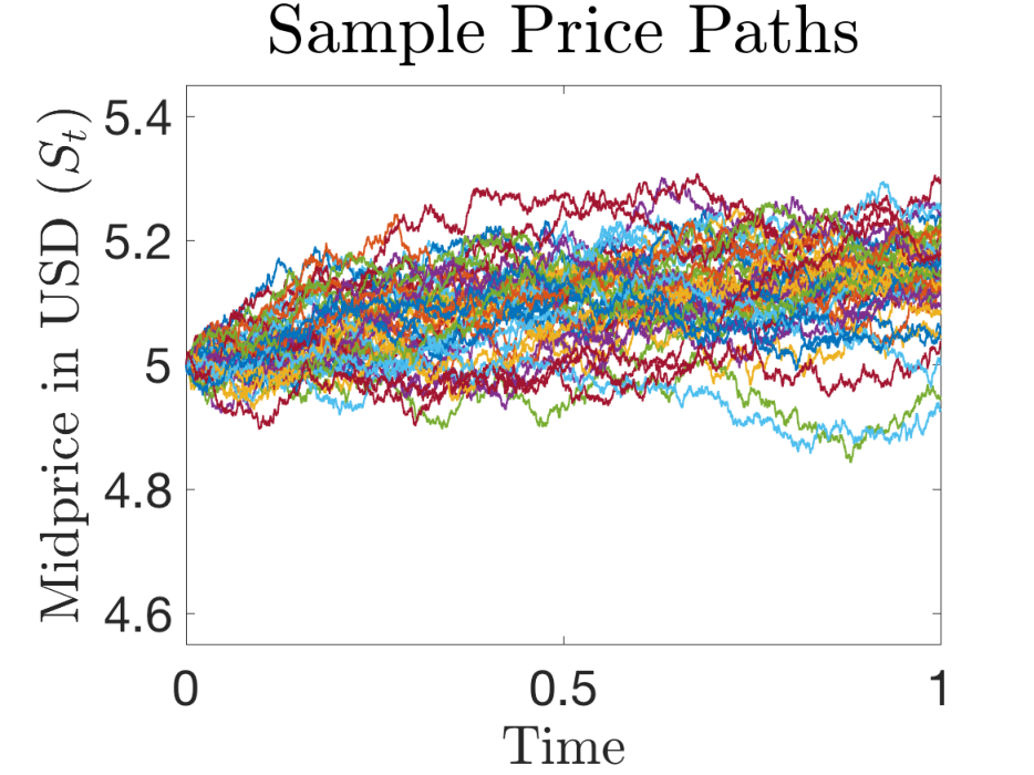
Refer to caption
Figure 2: Sample simulation paths with an Ornstein-Uhlenbeck process.

Figure 2 displays sample paths of the asset price and the filter. The top left plot demonstrates how the trader quickly detects the correct model based on the asset trajectory. In this simulation, the asset price initially drops, but then increases consistently. The posterior probability of model 1 adjusts accordingly, and initially rises, but then quickly drops and remains low. In the simulated path in the middle panel, the path of the midprice fluctuates around $5\$5 over the entire time period. The trader’s estimate for the posteriori probability of model 1 varies according to the price movements she is observing. The resulting strategy induced by the filter fluctuating is an advantage to the trader, because the fluctuating filter more accurately reflects the actual behaviour of the asset price path – as opposed to being certain that the true model is model 2. Finally, the bottom panel of the figure shows a collection of 4040 sample midprice path trajectories.

6.2 Mean-Reverting Pure Jump Process

In this section, we investigate the case where the trader begins with no inventory and aims to gain profits from her alpha model through the use of a round-trip trading strategy. The asset price is assumed to be completely driven by the market order-flow, so that there is no diffusion or drift in the unaffected midprice. We assume the asset price mean-reverts to some unknown level Θt\Theta_{t} which the trader must detect. More specifically, the asset midprice in USD satisfies the SDE

d​Ft=b⁡(d​Nt+−d​Nt−),dF_{t}=b\;(dN_{t}^{+}-dN_{t}^{-})\;, (6.3)

where Nt+N_{t}^{+} and Nt−N_{t}^{-} are doubly stochastic Poisson processes with intensities λt+\lambda^{+}_{t} and λt−\lambda_{t}^{-} defined by

λt+=μ+κ​(Θt−Ft)+​and ​λt−=μ+κ​(Θt−Ft)−,\lambda_{t}^{+}=\mu+\kappa\left(\Theta_{t}-F_{t}\right)_{+}\,\text{and }\,\lambda_{t}^{-}=\mu+\kappa\left(\Theta_{t}-F_{t}\right)_{-}\;, (6.4)

where (x)+(x)_{+} and (x)−(x)_{-} denote the positive and negative parts of xx, respectively.

We assume Θt\Theta_{t} is a Markov chain with generator matrix 𝑪\boldsymbol{C}, specified in Table 2. The filter for Θt\Theta_{t} cannot be computed explicitly, but it may be approximated via a Euler-Maruyama scheme of the SDE for the logarithm of the filter (see the SDE in Theorem 3.1). The resulting approximation for the value of the filter, given that the values of 𝑵{\boldsymbol{N}} have been observed at times {tk}k=1K\{t_{k}\}_{k=1}^{K}, where t0=0t_{0}=0 and tK=Tt_{K}=T is obtained via the recursive formula

Λt0j=π0j,\Lambda_{t_{0}}^{j}=\pi_{0}^{j}\;, (6.5a)
and
Λtk+1j=Λtkj​exp⁡{2​(1−μ−κ2​|θj−Ftk|)​Δk+1+∑i=1J(ΛtkiΛtkj)​Cj,i​Δk+1}×(μ+κ​(θj−Ftk)+)Δ​Ntk+1+×(μ+κ​(θj−Ftk)−)Δ​Ntk+1−,\begin{split}\Lambda_{t_{k+1}}^{j}=&\Lambda_{t_{k}}^{j}\exp\left\{2\left(1-\mu-\tfrac{\kappa}{2}\left\lvert\theta_{j}-F_{t_{k}}\right\rvert\right)\Delta_{k+1}+\sum_{i=1}^{J}\left(\frac{\Lambda_{t_{k}}^{i}}{\Lambda_{t_{k}}^{j}}\right)C_{j,i}\;\Delta_{k+1}\right\}\\ &\qquad\times\left(\mu+\kappa\left(\theta_{j}-F_{t_{k}}\right)_{+}\right)^{\Delta N_{t_{k+1}}^{+}}\times\left(\mu+\kappa\left(\theta_{j}-F_{t_{k}}\right)_{-}\right)^{\Delta N_{t_{k+1}}^{-}}\,,\end{split} (6.5b)

∀k≥1\forall k\geq 1, where Δ​Ntk±=Ntk±−Ntk−1±\Delta N_{t_{k}}^{\pm}=N_{t_{k}}^{\pm}-N_{t_{k-1}}^{\pm} and Δk=tk=tk−1\Delta_{k}=t_{k}=t_{k-1}. Alternatively, the trader’s filter for Θ\Theta may be found using the forward equations, which are discussed in more detail in D as well as in Section 7.1. The forward equation approach is recommended if the time-steps Δk\Delta_{k} are relatively large, which introduces inaccuracies into the above Euler-Maruyama approximation to the solution of the filtering SDE of Theorem 3.1.

We assume the trader has a one hour trading horizon, and completely unwinds her positions by the end of the trading period. The optimal control in this set-up can be found in closed form. Let us define the constant κ⋆=b​κ\kappa^{\star}=b\,\kappa and the J×JJ\times J matrix 𝑪⋆=𝑪+κ⋆​𝑰(J×J)\boldsymbol{C}^{\star}=\boldsymbol{C}+\kappa^{\star}\boldsymbol{I}_{(J\times J)}, where 𝑰(J×J)\boldsymbol{I}_{(J\times J)} represents the J×JJ\times J identity matrix. Let us also define the functions 𝚿1:[0,T]×ℝJ×J→ℝJ×J\boldsymbol{\Psi}_{1}:[0,T]\times\mathds{R}^{J\times J}\rightarrow\mathds{R}^{J\times J}, 𝚿2:[0,T]×ℝJ×J→ℝJ×J\boldsymbol{\Psi}_{2}:[0,T]\times\mathds{R}^{J\times J}\rightarrow\mathds{R}^{J\times J}, ψ1:[0,T]×ℝ→ℝ\psi_{1}:[0,T]\times\mathds{R}\rightarrow\mathds{R} and ψ2:[0,T]×ℝ→ℝ\psi_{2}:[0,T]\times\mathds{R}\rightarrow\mathds{R} where

𝚿1​(τ,𝒀)\displaystyle\boldsymbol{\Psi}_{1}(\tau,\;\boldsymbol{Y}) =(eτ​γ−e−τ​γ)−1​eτ​𝒀​(𝚿2​(τ,γ​𝑰(J×J)−𝒀)+𝚿2​(τ,−γ​𝑰(J×J)−𝒀)),\displaystyle=\left(e^{\tau\gamma}-e^{-\tau\gamma}\right)^{-1}e^{\tau\boldsymbol{Y}}\left(\,\boldsymbol{\Psi}_{2}(\tau,\;\gamma\,\boldsymbol{I}_{(J\times J)}-\boldsymbol{Y})+\boldsymbol{\Psi}_{2}(\tau,\;-\gamma\,\boldsymbol{I}_{(J\times J)}-\boldsymbol{Y})\,\right)\;,
𝚿2​(τ,𝒀)\displaystyle\boldsymbol{\Psi}_{2}(\tau,\;\boldsymbol{Y}) =𝒀−1​(eτ​𝒀−𝑰(J×J)),\displaystyle=\boldsymbol{Y}^{-1}\left(e^{\tau\boldsymbol{Y}}-\boldsymbol{I}_{(J\times J)}\right)\;,

and where ψ1\psi_{1} and ψ2\psi_{2} are the scalar versions of the functions above, defined as

ψ1​(τ,y)\displaystyle\psi_{1}(\tau,\;y) =(eτ​γ−e−τ​γ)−1​eτ​y​(ψ2​(τ,γ−y)+ψ2​(τ,−γ−y)), and\displaystyle=\left(e^{\tau\gamma}-e^{-\tau\gamma}\right)^{-1}e^{\tau y}\left(\,\psi_{2}(\tau,\;\gamma-y)+\psi_{2}(\tau,\;-\gamma-y)\right)\,,\text{ and}
ψ2​(τ,y)\displaystyle\psi_{2}(\tau,\;y) =y−1​(eτ​y−1).\displaystyle=y^{-1}\left(e^{\tau y}-1\right)\;.

The optimal trading speed for this set-up, letting α↑∞\alpha\uparrow\infty is

ν⋆​(t,F,Q,𝚲)=\displaystyle\nu^{\star}(t,F,Q,{\boldsymbol{\Lambda}})= −γ​coth⁡(γ⁡(T−t))​Q\displaystyle-\gamma\coth(\gamma\,(T-t))\,Q
+κ⋆[−Fψ1(T−t,κ⋆)+𝝅⊺(𝚲)Ψ1(T−t,𝑪)𝜽\displaystyle+\kappa^{\star}\Big[-F\;\psi_{1}(T-t,\,\kappa^{\star})+{\boldsymbol{\pi}}^{\intercal}({\boldsymbol{\Lambda}})\,\Psi_{1}(T-t,\,\boldsymbol{C})\,\boldsymbol{\theta}
−κ⋆𝝅⊺(𝚲)𝑪⋆−1(Ψ1(T−t,𝑪⋆)−ψ1(T−t,κ⋆)𝑰(J×J))𝜽],\displaystyle\hskip 20.00003pt\hskip 10.00002pt-\kappa^{\star}{\boldsymbol{\pi}}^{\intercal}({\boldsymbol{\Lambda}})\,{\boldsymbol{C}^{\star}}^{-1}\left(\Psi_{1}(T-t,\,\boldsymbol{C}^{\star})-\psi_{1}(T-t,\,\kappa^{\star})\boldsymbol{I}_{(J\times J)}\right)\boldsymbol{\theta}\Big]\;,

where in the above, 𝜽=(θj)j∈𝔍\boldsymbol{\theta}=(\theta_{j})_{j\in{\mathfrak{J}}} is a column vector containing all of the possible values that Θt\Theta_{t} can take.

In the numerical experiments, we assume two possible latent states for Θt\Theta_{t}: θ1=$4.9\theta_{1}=\$4.9 and θ2=$5.1\theta_{2}=\$5.1, and that the investor has an uninformed prior: π01=π02=0.5\pi_{0}^{1}=\pi_{0}^{2}=0.5. The remaining parameters are provided in Table 2. Note that we assume the latent process’s generator matrix is symmetric so the trader has no a priori preference for the asset’s price trajectory. The parameters for μ\mu, κ\kappa and 𝑪\boldsymbol{C} are all taken to be in the same range as the calibrated parameters for the 2-state model fit to Intel Corporation (INTC) stock data. These calibrated parameters are found in Section E, and are discussed in more detail in Section 7.1. The parameters found in Section E are on a per-second scale and those here are on a per-hour scale, so we must multiply them by 3600 to get those found in Table 2.

𝔑=0{\mathfrak{N}}=0, F0=$5F_{0}=\$5, b=$0.01b=\$0.01 ϕ=3×10⁻⁶,\phi=3\times 10^{-6}, 𝑪=[−101010−10]\boldsymbol{C}=\left[\begin{smallmatrix}-10&10\\ 10&-10\end{smallmatrix}\right],
κ=1077\kappa=1077, μ=481\mu=481, a=$10−5a=\$10^{-5}, β=$10−3\beta=\$10^{-3}.
Table 2: The parameters in the pure jump mean-reverting model. All of the time-sensitive parameters are defined on an hourly scale.
Refer to caption
Refer to caption
Refer to caption
Figure 3: Simulation Results with a Pure-Jump Mean-Reverting Process

For this simulation we fix a path for the latent process so that the value of Θt\Theta_{t} stays at $5.1\$5.1 over the period t∈[0,0.5]t\in[0,0.5] after which it jumps down to $4.9\$4.9 and remains there until the end of the trading period. This set-up will put the trader at a disadvantage. With the generator matrix defined in Table 2, the trader expects the latent process to jump an average of 10 times during the hour, whereas the path we fix for Θ\Theta jumps only once. Figure 3 shows the performance of the trader over the course of the hour. This implies that the trader will be acting based on the assumption that the latent process is on average 10 times more active than it is in the simultaion.

The top right portion of figure 3 demonstrates that on average, the filter detects the jump from Θt=$5.1\Theta_{t}=\$5.1 to Θt=$4.9\Theta_{t}=\$4.9. Furthermore, the bottom right panel shows the trader made a positive profit in 100%100\% of simulated scenarios. The left panels show heat maps of the trading speed (top left) and inventory (bottom left), respectively. Just as the strategy was constructed, the agent unwinds inventory by the end of the trading horizon. Moreover, she attains a short position initially, because she detects that Θt=$5.1\Theta_{t}=\$5.1 in the first half of the strategy, but expects the regime to switch causing a drop in asset price.

7 Model Calibration

This section shows how to calibrate the model in Section 2 to market data using maximum likelihood estimation (MLE) through the expectation-maximization (EM) algorithm. This procedure will simultaneously enable us to classify hidden states within historical data and determine what kind of dynamics governs the behaviour of the midprice and order-flow within each of the hidden states. The EM algorithm is based on Dempster et al. (1977) and the Baum-Welch algorithm (Baum et al., 1970). Once the general procedure is described, we apply it to calibrate a generalized version of the pure-jump mean-reverting model in Section 6.2.

7.1 The EM Algorithm

This section presents the discretized version of the asset and market dynamics in Section 2 and its associated calibration algorithm. We assume we observed DD independent paths (e.g., from several different days of trading within the same trading hour) of the process (F,𝑵,𝝀)\left(F,{\boldsymbol{N}},{\boldsymbol{\lambda}}\right) at discrete, uniformly spaced, times 𝒯={tk=Δt×k:k=0,…,K}\mathcal{T}=\left\{t_{k}={\Delta t\,}\times k:k=0,\dots,K\right\}, where Δ​t>0{\Delta t\,}>0 is the time interval in between observations.

Define the the discrete time processes Yk=(Ftk,𝑵tk,𝝀tk)Y_{k}=\left(F_{t_{k}},{\boldsymbol{N}}_{t_{k}},{\boldsymbol{\lambda}}_{t_{k}}\right) and Zk=ΘtkZ_{k}=\Theta_{t_{k}} for each tk∈𝒯t_{k}\in\mathcal{T}. Given the assumptions in Section 2, (Y,Z)={(Yk,Zk)}k=0​…​K(Y,Z)=\left\{(Y_{k},Z_{k})\right\}_{k=0\dots K} is a Markov process. Furthermore, the transition matrix of the process ZkZ_{k} and the distribution of Z0Z_{0} are known and can be written as

𝑷\displaystyle\boldsymbol{P} =[ℙ⁡(Zk=θj∣Zk−1=θi)]i,j=1J=eΔ​t​𝑪,and\displaystyle=\left[\mathbb{P}\left(Z_{k}=\theta_{j}\mid Z_{k-1}=\theta_{i}\right)\right]_{i,j=1}^{J}=e^{{\Delta t\,}\boldsymbol{C}},\hskip 20.00003pt\text{and} (7.1)
𝝅0\displaystyle\boldsymbol{\pi}_{0} =[ℙ⁡(Z0=θi)]i=1J=(π0i)i=1J.\displaystyle=\left[\mathbb{P}\left(Z_{0}=\theta_{i}\right)\right]_{i=1}^{J}=\left(\pi_{0}^{i}\right)_{{i=1}}^{J}\,. (7.2)

Moreover, by the definitions of the processes FF, N+N^{+}, N−N^{-} and Θ\Theta, the processes YY and ZZ inherit the conditional independence structure depicted in the directed graph shown in Figure 4. It is important to note that here we allow for dependence between the visible states YY even when conditioned on the latent states (i.e., there are connections between subsequent YY). This differs from the usual HMM setup where YY are conditionally independent when conditioned on ZZ.

Z0Z_{0}Z1Z_{1}𝑷\boldsymbol{P}Z2Z_{2}𝑷\boldsymbol{P}Z3Z_{3}𝑷\boldsymbol{P}Y0Y_{0}Y1Y_{1}fψf_{\psi}Y2Y_{2}fψf_{\psi}Y3Y_{3}fψf_{\psi}
Figure 4: Directed graphical representation of the price and order-flow model.

More specifically, we have

ℙ(Yk∈ℬ,Zk=θi∣Yk−1,Zk−1)=ℙ(Yk∈ℬ∣Yk−1,Zk−1)ℙ(Zk∣Zk−1),\mathbb{P}\left(\,Y_{k}\in{\mathcal{B}},Z_{k}=\theta_{i}\mid Y_{k-1},Z_{k-1}\,\right)=\mathbb{P}\left(Y_{k}\in{\mathcal{B}}\mid Y_{k-1},Z_{k-1}\,\right)\mathbb{P}\left(Z_{k}\mid Z_{k-1}\right)\;, (7.3)

for eack k=1​…​Kk=1\dots K and any Borel measurable set ℬ{\mathcal{B}}. Let us also assume the transition density for YkY_{k} conditional on (Yk−1,Zk−1)(Y_{k-1},Z_{k-1}) is known for each k=1,…,Kk=1,\dots,K, and that given a set of suitable parameters ψ\psi we can write

ℙ⁡(Yk∈d​y∣Yk−1=y0,Zk−1=θi)=fψ​(tk,y,tk−1,y0,θi)​𝝁​(d​y),\mathbb{P}\left(Y_{k}\in dy\mid Y_{k-1}=y_{0},Z_{k-1}=\theta_{i}\right)=f_{\psi}(t_{k},\,y\,;t_{k-1},y_{0},\theta_{i})\,{\boldsymbol{\mu}}(dy), (7.4)

where for each fixed (y0,θj)∈ℝ2​J+3×{θj}j∈𝔍(y_{0},\theta_{j})\in\mathds{R}^{2J+3}\bigtimes\left\{\theta_{j}\right\}_{j\in{\mathfrak{J}}}, and fixed times 0≤tk−1<tk≤T0\leq t_{k-1}<t_{k}\leq T, fψf_{\psi} is a probability density function, and where 𝝁{\boldsymbol{\mu}} is the Lebesgue measure. In machine learning language, the function fψf_{\psi} is often called the emission probability. It may be found by solving the appropriate Kolmogorov/Fokker-Planck forward equation. If we consider fψi​(t,y)=fψ​(t,y,s,y0,θi)f^{i}_{\psi}(t,y)=f_{\psi}(t,\,y\,;s,y_{0},\theta_{i}) for fixed values of y0y_{0} and for 0≤s≤t≤T0\leq s\leq t\leq T, then fψif^{i}_{\psi} is the solution to the PDE

{(∂t+∑j∈𝔍(et​𝑪)i,jℒ^†j)fiψ(t,y)=0fψi​(s,y)=δ⁡(y−y0),,\begin{cases}(\,\partial_{t}+\sum_{j\in{\mathfrak{J}}}\left(e^{t\,\boldsymbol{C}}\right)_{i,j}\widehat{\mathcal{L}}^{\dagger}_{j}\;)f^{i}_{\psi}(t,y)=0\\ f^{i}_{\psi}(s,y)=\delta(y-y_{0})\,,\end{cases}\;, (7.5)

where δ⁡(y)\delta(y) is the dirac delta function, and the operator ℒ^j†\widehat{\mathcal{L}}^{\dagger}_{j} is the adjoint infinitesimal generator of the process Yt=(Ft,𝑵t,𝝀t)Y_{t}=\left(F_{t},{\boldsymbol{N}}_{t},{\boldsymbol{\lambda}}_{t}\right) conditional on the event {ω:Zt(ω)=θj,∀t∈[0,T]}\{\omega:Z_{t}(\omega)=\theta_{j},\forall t\in[0,T]\}, and where (et​𝑪)i,j\left(e^{t\,\boldsymbol{C}}\right)_{i,j} is element (i,j)(i,j) of the matrix exponential of t​𝑪t\,\boldsymbol{C}. In practice, it is possible to use any number of approximations to obtain the emission probability density.

In the remainder of this section we use the notation YkdY_{k}^{d} and ZkdZ_{k}^{d} to denote the processes YY and ZZ, observed at time tkt_{k} in the dthd^{\text{th}} independently observed path. We also introduce the notation 𝒴m:nd≜⋂m≤k≤n{ω:Ykd∈dykd}\mathcal{Y}_{m:n}^{d}\triangleq\bigcap_{m\leq k\leq n}\left\{\omega:Y_{k}^{d}\in dy_{k}^{d}\right\} where each {ω:Ykd∈d​ykd}\left\{\omega:Y_{k}^{d}\in dy_{k}^{d}\right\}, represents the event in which we observe the visible process YkdY_{k}^{d} having taken the value ykdy_{k}^{d}.

The objective is to find the set of parameters Γ=(π0,𝑷,ψ)∈𝔊\Gamma=(\pi_{0},\boldsymbol{P},\psi)\in\mathfrak{G} which maximize the likelihood of having made observations {ykd}k,d=1K,D\{y_{k}^{d}\}_{k,d=1}^{K,D} of the process YY, where 𝔊\mathfrak{G} is the set of allowable parameters, defined as

𝔊={𝝅=(πi)t∈[0,T]J∈ℝJ: 1J⊺𝝅=1,πi∈[0,1]}×{𝑷=(Pi,j)t∈[0,T]J∈ℝJ×J: 1⊺J𝑷=𝟏J,Pi,j∈[0,1]}×𝔊ψ,\begin{split}\mathfrak{G}=&\left\{\boldsymbol{\pi}=\left(\pi_{i}\right)_{{t\in[0,T]}}^{J}\in\mathds{R}^{J}\,:\,\boldsymbol{1}_{J}^{\intercal}\boldsymbol{\pi}=1,\pi_{i}\in[0,1]\right\}\\ &\quad\bigtimes\left\{\boldsymbol{P}=\left(P_{i,j}\right)_{{t\in[0,T]}}^{J}\in\mathds{R}^{J\times J}\,:\,\boldsymbol{1}^{\intercal}_{J}\boldsymbol{P}=\boldsymbol{1}_{J},P_{i,j}\in[0,1]\right\}\bigtimes\mathfrak{G}_{\psi}\;,\end{split} (7.6)

where 𝟏J\boldsymbol{1}_{J} is a column vector of ones, and 𝔊ψ\mathfrak{G}_{\psi} is the set on which we restrict ψ\psi. The first two sets in the definition of 𝔊\mathfrak{G} ensure the entries of 𝝅0\boldsymbol{\pi}_{0} sum to one, and 𝑷\boldsymbol{P} is a valid Markov chain transition matrix, respectively.

Due to the presence of the unobserved (latent) states ZZ, the number of terms in the log-likelihood of the discrete observations of the process YY grows exponentially with the number of observations. It is, therefore, necessary to use the EM algorithm which provides a sequence of improving parameter estimates {Γk}k=1∞\{\Gamma_{k}\}_{k=1}^{\infty}. Each term in the sequence has larger likelihood than the previous.

The EM algorithm proceeds as follows. Begin with an initial guess (e.g., as estimated from an equivalent model with no latent states) for the model parameters, Γ0∈𝔊\Gamma_{0}\in\mathfrak{G}. Generate a recursive sequence of parameters {Γn}n=1∞\{\Gamma_{n}\}_{n=1}^{\infty}, defined by the relationship

Γn+1=argsupΓ∈𝔊𝔼ℙΓn[logLΓ|{𝒴0:Kd}d=1D],\Gamma_{n+1}=\arg\sup_{\Gamma\in\mathfrak{G}}\;\mathbb{E}^{\mathbb{P}^{\Gamma_{n}}}\left[\;\left.\log L^{\Gamma}\;\right|\;\{\mathcal{Y}_{0:K}^{d}\}_{d=1}^{D}\right]\;, (7.7)

where log⁡LΓ\log L^{\Gamma} is the joint log-likelihood of having observed DD independent paths of the process (Y,Z)(Y,Z) given the parameter set Γ\Gamma, and where ℙΓn\mathbb{P}^{\Gamma_{n}} is the probability measure conditional on the dynamics of (Y,Z)(Y,Z) having parameters Γn\Gamma_{n}. The joint log-likelihood for our model yields the decomposition

log⁡LΓ=∑d=1D∑i=1Jlog(π0i) 1{Z0d=θi}+∑d=1D∑k=0K−2∑i,j=1Jlog(Pi,j) 1{Zkd=θi,Zk+1d=θj}+∑d=1D∑k=0K−1∑i=1Jlog(fψ(tk+1,yk+1d;tk,ykd,θi)) 1{Zkd=θi}.\begin{split}\log L^{\Gamma}=&\phantom{+}\sum_{d=1}^{D}\sum_{i=1}^{J}\log\left(\pi_{0}^{i}\right)\,\mathds{1}_{\left\{{{Z_{0}^{d}=\theta_{i}}}\right\}}\\ &+\sum_{d=1}^{D}\sum_{k=0}^{K-2}\sum_{i,j=1}^{J}\log\left(P_{i,j}\right)\,\mathds{1}_{\left\{{{Z_{k}^{d}=\theta_{i}},\,{Z_{k+1}^{d}=\theta_{j}}}\right\}}\\ &+\sum_{d=1}^{D}\sum_{k=0}^{K-1}\sum_{i=1}^{J}\log\left(f_{\psi}(t_{k+1},y_{k+1}^{d};t_{k},y_{k}^{d},\theta_{i})\right)\,\mathds{1}_{\left\{{{Z_{k}^{d}=\theta_{i}}}\right\}}\;.\end{split} (7.8)

We then have

𝔼ℙΓn[logLΓ∣𝒴0:K1,…,𝒴0:KD]=\displaystyle\mathbb{E}^{\mathbb{P}^{\Gamma_{n}}}\left[\log L^{\Gamma}\mid\mathcal{Y}_{0:K}^{1},\dots,\mathcal{Y}_{0:K}^{D}\right]= ∑d=1D∑i=1Jlog⁡(π0i)​γ0i,d\displaystyle\sum_{d=1}^{D}\sum_{i=1}^{J}\log\left(\pi_{0}^{i}\right)\,\gamma_{0}^{i,d} (7.9)
+∑d=1D∑k=0K−2∑i,j=1Jlog(Pi,j)ξki,j,d\displaystyle+\sum_{d=1}^{D}\sum_{k=0}^{K-2}\sum_{i,j=1}^{J}\log\left(P_{i,j}\right)\,\xi_{k}^{i,j,d}
+∑d=1D∑k=0K−1∑i=1Jlog(fψ(tk+1,yk+1d;tk,ykd,θi))γki,d,\displaystyle+\sum_{d=1}^{D}\sum_{k=0}^{K-1}\sum_{i=1}^{J}\log\left(f_{\psi}(t_{k+1},y_{k+1}^{d};t_{k},y_{k}^{d},\theta_{i})\right)\,\gamma_{k}^{i,d}\;,

where the smoother γki,d\gamma_{k}^{i,d} and two-slice marginal ξki,j,d\xi_{k}^{i,j,d} are defined as

γki,d=ℙΓn(Zkd=θi|𝒴0:Kd) and ξki,j,d=ℙΓn(Zkd=θi,Zk+1d=θj|𝒴0:Kd).\displaystyle\gamma_{k}^{i,d}=\mathbb{P}^{\Gamma_{n}}\!\left({Z_{k}^{d}=\theta_{i}}\,|\,\mathcal{Y}_{0:K}^{d}\right)\;\hskip 10.00002pt\text{ and }\hskip 10.00002pt\xi_{k}^{i,j,d}=\mathbb{P}^{\Gamma_{n}}\!\left({Z_{k}^{d}=\theta_{i}},{Z_{k+1}^{d}=\theta_{j}}\,|\,\mathcal{Y}_{0:K}^{d}\right)\;. (7.10)

These coefficients can be computed by using the forward-backward algorithm, which, for our model, is provided in D. Next, because each line of equation (7.9) depends only on one of 𝝅0\boldsymbol{\pi}_{0}, 𝑷\boldsymbol{P}, and ψ\psi, the updated estimates for the parameters can be obtained independently. The resulting update rules (which maximize (7.9)) are

π0j⋆\displaystyle\pi_{0}^{j\,\star} =1D​∑d=1Dγ0j,d,\displaystyle=\tfrac{1}{D}\sum_{d=1}^{D}\gamma_{0}^{j,d}, j∈𝔍,\displaystyle j\in{\mathfrak{J}}, (7.11a)
Pi,j⋆\displaystyle P_{i,j}^{\star} =∑d=1D∑k=0K−2ξki,j,d∑d=1D∑k=0K−2∑j=1Jξki,j,d,\displaystyle=\frac{\sum_{d=1}^{D}\sum_{k=0}^{K-2}\xi_{k}^{i,j,d}}{\sum_{d=1}^{D}\sum_{k=0}^{K-2}\sum_{j=1}^{J}\xi_{k}^{i,j,d}}, i,j∈𝔍,\displaystyle i,j\in{\mathfrak{J}}, (7.11b)
ψ⋆\displaystyle\psi^{\star} =arg⁡maxψ∈𝔊ψ​{∑d=1D∑k=0K−1∑i=1Jlog⁡(fψ​(tk+1,yk+1d,tk,ykd,θi))​γki,d}.\displaystyle=\arg\max_{\psi\in\mathfrak{G}_{\psi}}\left\{\sum_{d=1}^{D}\sum_{k=0}^{K-1}\sum_{i=1}^{J}\log\left(f_{\psi}(t_{k+1},y_{k+1}^{d};t_{k},y_{k}^{d},\theta_{i})\right)\,\gamma_{k}^{i,d}\right\}. (7.11c)

Hence, Γn+1=(𝝅0⋆,𝑷⋆,ψ⋆)\Gamma_{n+1}=\left(\boldsymbol{\pi}_{0}^{\star},\boldsymbol{P}^{\star},\psi^{\star}\right). The updated estimates for the emission probabilities (7.11c), may in some models be analytically tractable (e.g., gaussian mixtures, or discrete distributions), while in others one may have to resort to numerical optimization schemes.

More details on the maximization of equation (7.7) and of various other related computational concerns are outlined in Rabiner (1989). The one subtle difference between the model presented in this section and the classical Hidden Markov Model, such as the one found in Rabiner (1989) is that the visible process YY exhibits temporal correlation even when conditioning on the path of the hidden process ZZ.

7.2 Mean-Reverting Pure-Jump Model

In this section, we show how to implement the EM algorithm for the model presented in section 6.2. Assuming that the observations are frequent enough to observe one or no jumps in the midprice, we adopt a censored version of the model. As in Section 6.2, we assume the increments of the midprice FtF_{t} in the interval [tn,tn+1)[t_{n},t_{n+1}) satisfy

Ftn+1−Ftn=b⁡(Δ​Ntn+−Δ​Ntn−),F_{t_{n+1}}-F_{t_{n}}=b\left(\Delta N_{t_{n}}^{+}-\Delta N_{t_{n}}^{-}\right), (7.12)

where each of the Δ​Nt±∈{0,1}\Delta N_{t}^{\pm}\in\left\{0,1\right\} are censored, conditionally independent Poisson random variables with respective stochastic rate parameters λt+​Δ​t\lambda_{t}^{+}{\Delta t\,} and λt+​Δ​t\lambda_{t}^{+}{\Delta t\,}, where

λt±=∑j=1Jλt±,j𝟙{Θtj=θj},\lambda_{t}^{\pm}=\sum_{j=1}^{J}\lambda_{t}^{\pm,j}\mathds{1}_{\left\{{\Theta_{t}^{j}=\theta_{j}}\right\}}\;, (7.13)

and we assume λt±,j\lambda_{t}^{\pm,j} have constant paths over each observation period (this can easily be relaxed). Moreover,

λtn+,j=μj+κj​(θj−Ftn)+andλtn−,j=μj+κj​(θj−Ftn)−.\lambda_{t_{n}}^{+,j}=\mu_{j}+\kappa_{j}\left(\theta_{j}-F_{t_{n}}\right)_{+}\hskip 10.00002pt\text{and}\hskip 10.00002pt\lambda_{t_{n}}^{-,j}=\mu_{j}+\kappa_{j}\left(\theta_{j}-F_{t_{n}}\right)_{-}\;. (7.14)

This generalizes the model in Section 6.2 as all parameters μ\mu, θ\theta and κ\kappa may vary according to the state of the hidden process Θt\Theta_{t}. The emission probabilities have parameters ψ={μj​κj,θj}j=1J\psi=\left\{\mu_{j}\,\kappa_{j},\theta_{j}\right\}_{j=1}^{J}, which represent (within each state) the base noise level, the mean reversion rate, and the mean reversion level of the mid-price, respectively. With these ingredients, we can now state the emission probability as follows

fψ​(tk+1,Yk+1,tk,Yk,θj)={e−Δ​t​λtk−,j​(1−e−Δ​t​λtk+,j), if ​Ftn+1>Ftke−Δ​t​λtk+,j​(1−e−Δ​t​λtk−,j), if ​Ftn+1<Ftke−Δ​t​(λtk+,j+λt−,j)+(1−e−Δ​t​λtk+,j)​(1−e−Δ​t​λtk−,j),otherwise.\begin{split}&f_{\psi}(t_{k+1},Y_{k+1};t_{k},Y_{k},\theta_{j})\\ &=\begin{cases}e^{-{\Delta t\,}\lambda^{-,j}_{t_{k}}}\left(1-e^{-{\Delta t\,}\lambda^{+,j}_{t_{k}}}\right),&\text{ if }F_{t_{n+1}}>F_{t_{k}}\\ e^{-{\Delta t\,}\lambda^{+,j}_{t_{k}}}\left(1-e^{-{\Delta t\,}\lambda^{-,j}_{t_{k}}}\right),&\text{ if }F_{t_{n+1}}<F_{t_{k}}\\ e^{-{\Delta t\,}\left(\lambda^{+,j}_{t_{k}}+\lambda^{-,j}_{t}\right)}+\left(1-e^{-{\Delta t\,}\lambda^{+,j}_{t_{k}}}\right)\left(1-e^{-{\Delta t\,}\lambda^{-,j}_{t_{k}}}\right),&\;\text{otherwise.}\end{cases}\end{split} (7.15)

Armed with this expression, we can apply the EM algorithm from Section 7.1 to obtain parameter estimates. In this model, we cannot obtain explicit updates for ψ\psi from (7.11c), and instead use a numerical optimization.

7.3 Example Fit to INTC stock Data

In this section, we fit the model presented in Section 7.2 to intraday price data. We fit this model to the midprice of INTC stock on the NASDAQ exchange taken at each second between the hours of 10:00 and 11:00 on each business day during 2014. To normalize this data between days, we subtract the price at 10:00 on the same day from each data point, so that we are fitting the model from Section 7.2 to the price change in INTC since 10:00 on each day. Moreover, we assume that price paths are independent across days. From this dataset, we set Δ​t=1{\Delta t\,}=1, so that all of the parameter estimates can be interpreted on a per-second scale. In E we show the parameter estimates for the model with 11 to 66 latent states. All of these parameter estimates were obtained using the EM algorithm described in Section 7.1 applied to the censored pure jump model in Section 7.2.

An important part of calibrating models with latent states is to estimate the possible number of states that a model should have. To choose an ‘optimal’ number of latent states we use two information criteria: the Bayesian Information Criterion (BIC), and the integrated completed likelihood (ICL). For the purposes of our paper, we use an approximation to the ICL which can be found in Biernacki et al. (2000). The definitions of both of these criteria and some related computational details can be found in E. It is well known that ICL typically under-estimates the true number of latent states, whereas the BIC typically over estimates the number of latent states. For INTC, BIC and ICL estimate 5 and 1 latent states, respectively. This implies that the true number of of states should be somewhere within that range.

Recall that μi\mu_{i}, κi\kappa_{i} and θi\theta_{i} can be interpreted as the noise level, the mean-reversion rate, and the mean-reversion level, respectively. We find that the mean-reversion level does not vary much (all less than 3​¢3\cent in absolute value) in comparison to realized daily stock price movements which can range anywhere in between −50​¢-50\cent to 50​¢50\cent. This indicates the daily asset prices typically mean-revert back to their initial values no matter the state of the latent process. The distinction between states occurs in the strength of the mean-reversion through κi\kappa_{i}, and the base noise level μi\mu_{i}.

The estimates for the transition probabilities shown in E indicate there is persistence in the latent process regardless of the number of latent states. This implies the trader is able to detect market states and to act on them before the states switch again. From the estimated generator matrices in E, the mean time spent in a given state can range from a few seconds to over 800800 seconds, depending on the number of allowed latent states.

8 Conclusion

In this paper, we solved a finite horizon optimal trading problem in which the midprice of the asset contains a latent alpha component stemming from a diffusive drift as well as a pure jump component. We obtain the solution in closed form, up to the computation of an expectation which depends on the class of potential models. The optimal trading speed is found to be a combination of the classical AC trading strategy plus a modulating term that incorporates the trader’s estimate of the latent factors and its forecast. The form of the solution is similar in spirit to the results in  Cartea and Jaimungal (2016) where the authors have an alpha component stemming from market order-flow, but in that work viewed as visible. We presented two examples one where the trader wishes to completely liquidate a large position (the optimal execution problem) and the other where the trader uses the latent states to generate a statistical arbitrage trading strategy. Both examples show that there is significant value in incorporating latent states. Finally, we presented a method for obtaining parameter estimates from data using the EM algorithm and applied it to an example stock.

There are many potential future directions left open for investigation. One direction which we have already been investigated is to generalize the analysis to trading multiple assets, as well as incorporating multiple latent factors. In this work, the trader is assumed to execute trades continuously and uses market orders which walk the limit order book (LOB) and hence obtain a temporary price impact. It would be interesting to analyze the case of executing market orders at discrete times, and hence recast the problem as an impulse control problem with latent alpha factors. Along similar lines, the agent may wish to use limit orders to squeeze even more profits out of the strategy. Combining market and limit orders, along the lines of Cartea and Jaimungal (2015) and Huitema (2013), but including latent alpha factors would also be quite interesting.

Appendix A Proof of Theorem 3.1

Proof.

We present here the proof of the case where σ>0\sigma>0. The case where σ=0\sigma=0 and A:=0A:=0 can be derived in the same fashion by excluding all of the diffusive terms.

Due to the Novikov Condition (3.1), we may define the measure ℚ\mathbb{Q} through the Radon-Nikodym derivative

(d​ℚd​ℙ)t\displaystyle\left(\frac{d\mathbb{Q}}{d\mathbb{P}}\right)_{t} =exp{−σ−1∫0tAu−dWu−σ−22∫0t(Au−)2du}\displaystyle=\exp\left\{-\sigma^{-1}\int_{0}^{t}A_{u-}\,dW_{u}-\frac{\sigma^{-2}}{2}\int_{0}^{t}\left(A_{u-}\right)^{2}du\right\}
×exp⁡{∫0t(λu−+−1)​𝑑u−∫0tlog⁡(λu−+)​d​Nu+}\displaystyle\times\exp\left\{\int_{0}^{t}(\lambda_{u-}^{+}-1)du-\int_{0}^{t}\log(\lambda_{u-}^{+})dN^{+}_{u}\right\}
×exp⁡{∫0t(λu−−−1)​𝑑u−∫0tlog⁡(λu−−)​d​Nu−},\displaystyle\times\exp\left\{\int_{0}^{t}(\lambda_{u-}^{-}-1)du-\int_{0}^{t}\log(\lambda_{u-}^{-})dN^{-}_{u}\right\}\;,

which is defined so that under the measure ℚ\mathbb{Q}, the process σ−1​(Ft−b⁡(Nt+−Nt−))\sigma^{-1}(F_{t}-b(N_{t}^{+}-N_{t}^{-})) is a Brownian Motion and both Nt+N_{t}^{+} and Nt−N_{t}^{-} have intensity process equal to 1. This measure is deliberately chosen so that FtF_{t}, Nt+N_{t}^{+} and Nt−N_{t}^{-} are ℚ\mathbb{Q}-independent of Θt\Theta_{t}. Additionally, the inverse of this Radon-Nikodym derivative is

(d​ℙd​ℚ)t=ζt\displaystyle\left(\frac{d\mathbb{P}}{d\mathbb{Q}}\right)_{t}=\zeta_{t} =exp⁡{σ−2​∫0tAu−​(d​Fu−b⁡(d​Nt+−d​Nt−))−σ−22​∫0t(Au−)2​du}\displaystyle=\exp\left\{{\sigma^{-2}\int_{0}^{t}A_{u-}(dF_{u}-b\>(dN_{t}^{+}-dN_{t}^{-}))-\frac{\sigma^{-2}}{2}\int_{0}^{t}\left(A_{u-}\right)^{2}du}\right\} (A.1)
×exp⁡{∫0t(1−λu−+)​du+∫0tlog⁡(λu−+)​d​Nu+}\displaystyle\times\exp\left\{\int_{0}^{t}(1-\lambda_{u-}^{+})du+\int_{0}^{t}\log(\lambda_{u-}^{+})dN^{+}_{u}\right\}
×exp⁡{∫0t(1−λu−−)​du+∫0tlog⁡(λu−−)​d​Nu−}.\displaystyle\times\exp\left\{\int_{0}^{t}(1-\lambda_{u-}^{-})du+\int_{0}^{t}\log(\lambda_{u-}^{-})dN^{-}_{u}\right\}\;.

Using these last two expressions, we can re-write the filter in terms of ℚ\mathbb{Q} expected values to obtain

πtj\displaystyle\pi_{t}^{j} =𝔼ℚ[𝟙{Θt=θj}ζt∣ℱt]𝔼ℚ​[ζt∣ℱt]\displaystyle=\frac{\mathbb{E}^{\mathbb{Q}}\left[\mathds{1}_{\left\{{\Theta_{t}=\theta_{j}}\right\}}\zeta_{t}\mid{\mathcal{F}}_{t}\right]}{\mathbb{E}^{\mathbb{Q}}\left[\zeta_{t}\mid{\mathcal{F}}_{t}\right]} (A.2)
=𝔼ℚ[𝟙{Θt=θj}ζt∣ℱt]∑i=1J𝔼ℚ[𝟙{Θt=θi}ζt∣ℱt]\displaystyle=\frac{\mathbb{E}^{\mathbb{Q}}\left[\mathds{1}_{\left\{{\Theta_{t}=\theta_{j}}\right\}}\zeta_{t}\mid{\mathcal{F}}_{t}\right]}{\sum_{i=1}^{J}\mathbb{E}^{\mathbb{Q}}\left[\mathds{1}_{\left\{{\Theta_{t}=\theta_{i}}\right\}}\zeta_{t}\mid{\mathcal{F}}_{t}\right]} (A.3)
=Λtj∑i=1JΛti.\displaystyle=\frac{\Lambda_{t}^{j}}{\sum_{i=1}^{J}\Lambda_{t}^{i}}\;. (A.4)

Next, we will attempt to find an SDE for each Λtj\Lambda_{t}^{j} term. This can be done by first defining the process δtj=𝟙{Θt=θj}\delta_{t}^{j}=\mathds{1}_{\left\{{\Theta_{t}=\theta_{j}}\right\}}, which satisfies the SDE

d​δtj=∑i=1Jδt−i​Cj,i​d​t+d​ℳ~tj,d\delta_{t}^{j}=\sum_{i=1}^{J}\delta_{t-}^{i}C_{j,i}\>dt+d\mathcal{\tilde{M}}_{t}^{j}\;,

under the measure ℚ\mathbb{Q}, where ℳ~tj\mathcal{\tilde{M}}_{t}^{j} is a square-integrable, 𝒢t{\mathcal{G}}_{t}–adapted, ℚ\mathbb{Q}-martingale and 𝑪\boldsymbol{C} is the generator matrix for Θt\Theta_{t}. All that’s left to compute the dynamics of the Λtj\Lambda_{t}^{j} is to figure out the dynamics of ζt​δtj\zeta_{t}\delta_{t}^{j} and then take the appropriate ℚ\mathbb{Q} expected value while conditioning on ℱt{\mathcal{F}}_{t}. The process δtj​ζt\delta_{t}^{j}\zeta_{t} satisfies the SDE

d⁡(ζt​δtj)\displaystyle d\left(\zeta_{t}\delta_{t}^{j}\right) =(ζt−​δt−j)​(σ−2​At−j​(d​Ft−b⁡(d​Nt+−d​Nt−))CLOSE\displaystyle=\left(\zeta_{t-}\delta_{t-}^{j}\right)\Bigg(\sigma^{-2}A_{t-}^{j}\;(dF_{t}-b(dN_{t}^{+}-dN_{t}^{-}))
OPEN+(λt−+−1)​(d​Nt+−d​t)+(λt−−−1)​(d​Nt−−d​t))\displaystyle\hskip 42.67912pt+(\lambda_{t-}^{+}-1)(dN_{t}^{+}-dt)+(\lambda_{t-}^{-}-1)(dN_{t}^{-}-dt)\Bigg)
+∑i=1Jζt−δt−iCj,idt+dℳtj\displaystyle\hskip 42.67912pt+\sum_{i=1}^{J}\zeta_{t-}\delta_{t-}^{i}C_{j,i}\;dt+d\mathcal{M}_{t}^{j}
=(ζt−​δt−j)​(σ−2​At−j​(d​Ft−b⁡(d​Nt+−d​Nt−))CLOSE\displaystyle=\left(\zeta_{t-}\delta_{t-}^{j}\right)\Bigg(\sigma^{-2}A_{t-}^{j}\;(dF_{t}-b(dN_{t}^{+}-dN_{t}^{-}))
OPEN+(λt−+,j−1)​(d​Nt+−d​t)+(λt−−,j−1)​(d​Nt−−d​t))\displaystyle\hskip 42.67912pt+(\lambda_{t-}^{+,j}-1)(dN_{t}^{+}-dt)+(\lambda_{t-}^{-,j}-1)(dN_{t}^{-}-dt)\Bigg)
+∑i=1Jζt−δt−iCj,idt+dℳtj,\displaystyle\hskip 42.67912pt+\sum_{i=1}^{J}\zeta_{t-}\delta_{t-}^{i}C_{j,i}\;dt+d\mathcal{M}_{t}^{j}\;,

where ℳtj\mathcal{M}_{t}^{j} is another square-integrable, 𝒢t{\mathcal{G}}_{t}–adapted, ℚ\mathbb{Q}-martingale.

Now we re-write the expression for Λtj\Lambda_{t}^{j} as the expected value of a stochastic integral

Λtj=𝔼ℚ[\displaystyle\Lambda_{t}^{j}=\mathbb{E}^{\mathbb{Q}}\Bigg[ δtjζt∣ℱt]\displaystyle\delta_{t}^{j}\zeta_{t}\mid{\mathcal{F}}_{t}\Bigg] (A.5)
=𝔼ℚ[\displaystyle=\mathbb{E}^{\mathbb{Q}}\Bigg[ (ζ0​δ0j)+∫0t(ζu−​δu−j)​(σ−2​Au−j​(d​Fu−b⁡(d​Nu+−d​Nu−)))\displaystyle\left(\zeta_{0}\delta_{0}^{j}\right)+\int_{0}^{t}\left(\zeta_{u-}\delta_{u-}^{j}\right)\bigg(\sigma^{-2}A_{u-}^{j}\;(dF_{u}-b(dN_{u}^{+}-dN_{u}^{-}))\bigg) (A.6)
+\displaystyle+ ∫0t(ζu−​δu−j)​(λu−+,j−1)​(d​Nu+−𝑑u)+∫0t(ζu−​δu−j)​(λu−−,j−1)​(d​Nu−−𝑑u)\displaystyle\int_{0}^{t}\left(\zeta_{u-}\delta_{u-}^{j}\right)(\lambda_{u-}^{+,j}-1)(dN_{u}^{+}-du)+\int_{0}^{t}\left(\zeta_{u-}\delta_{u-}^{j}\right)(\lambda_{u-}^{-,j}-1)(dN_{u}^{-}-du)
+\displaystyle+ ∫0t(∑i=1Jζu−δu−iCj,idu+dℳuj)|ℱt].\displaystyle\int_{0}^{t}\left(\sum_{i=1}^{J}\zeta_{u-}\delta_{u-}^{i}C_{j,i}\;du+d\mathcal{M}_{u}^{j}\right)\Biggr\rvert{\mathcal{F}}_{t}\Bigg]\;.

At this point we will need conditions guaranteeing that we can exchange the order of integration, in the expression above. First, by the definition of Λtj\Lambda_{t}^{j},

𝔼ℚ​[ζ0​δ0j∣ℱt]=π0j,\mathbb{E}^{\mathbb{Q}}\left[\zeta_{0}\delta_{0}^{j}\mid{\mathcal{F}}_{t}\right]=\pi_{0}^{j}\;, (A.7)

which allows us to replace the first term in (A.6). We can use the fact that Ft−F0−b⁡(Nt+−Nt−)=WtℚF_{t}-F_{0}-b(N_{t}^{+}-N_{t}^{-})=W_{t}^{\mathbb{Q}} is a ℚ\mathbb{Q}-Brownian motion to write

𝔼ℚ​[∫0t(ζu−​δu−j)​σ−2​Au−j​d​Wuℚ∣ℱt].\mathbb{E}^{\mathbb{Q}}\left[\int_{0}^{t}\left(\zeta_{u-}\delta_{u-}^{j}\right)\sigma^{-2}A_{u-}^{j}\;dW_{u}^{\mathbb{Q}}\mid{\mathcal{F}}_{t}\right]\;. (A.8)

Applying (Wong and Hajek, 1985, Chapter VI, Lemma 3.2), whose conditions are met with the bound (3.1), we can exchange the order of integration in the above term to get

∫0tΛu−j​σ−2​Au−j​d​Wuℚ.\int_{0}^{t}\Lambda_{u-}^{j}\sigma^{-2}A_{u-}^{j}\;dW_{u}^{\mathbb{Q}}\;. (A.9)

For the third and fourth terms, let us note that if we let 𝒰t±={u∈[0,t]:Nu±>Nu−±}\mathcal{U}^{\pm}_{t}=\left\{u\in[0,t]:N_{u}^{\pm}>N_{u-}^{\pm}\right\}, then by condition (3.1) we know 𝒰±\mathcal{U}^{\pm} is almost surely finite and ℱt{\mathcal{F}}_{t}-measurable. Therefore

𝔼ℚ​[∫0t(ζu−​δu−j)​(λu−±,j−1)​d​Nu±∣ℱt]\displaystyle\mathbb{E}^{\mathbb{Q}}\left[\int_{0}^{t}\left(\zeta_{u-}\delta_{u-}^{j}\right)(\lambda_{u-}^{\pm,j}-1)dN_{u}^{\pm}\mid{\mathcal{F}}_{t}\right] =𝔼ℚ​[∑u∈𝒰t±(ζu−​δu−j)​(λu−±,j−1)​(Nu±−Nu−±)∣ℱt]\displaystyle=\mathbb{E}^{\mathbb{Q}}\left[\sum_{u\in\mathcal{U}^{\pm}_{t}}\left(\zeta_{u-}\delta_{u-}^{j}\right)(\lambda_{u-}^{\pm,j}-1)(N_{u}^{\pm}-N_{u-}^{\pm})\mid{\mathcal{F}}_{t}\right] (A.10)
=∑u∈𝒰t±Λu−j​(λu−±,j−1)​(Nu±−Nu−±)\displaystyle=\sum_{u\in\mathcal{U}^{\pm}_{t}}\Lambda_{u-}^{j}(\lambda_{u-}^{\pm,j}-1)(N_{u}^{\pm}-N_{u-}^{\pm}) (A.11)
=∫0tΛu−j​(λu−±,j−1)​d​Nt±.\displaystyle=\int_{0}^{t}\Lambda_{u-}^{j}(\lambda_{u-}^{\pm,j}-1)dN_{t}^{\pm}\;. (A.12)

We can apply Fubini’s theorem on the remaining Riemann integral because the integrands are square integrable to exchange the order of integration and get

𝔼ℚ​[∫0t(∑i=1Jζu−​δu−i​Cj,i−(ζu−​δu−j)​(λu−+,j+λu−−,j−2))​𝑑u∣ℱt]\displaystyle\mathbb{E}^{\mathbb{Q}}\left[\int_{0}^{t}\left(\sum_{i=1}^{J}\zeta_{u-}\delta_{u-}^{i}C_{j,i}-\left(\zeta_{u-}\delta_{u-}^{j}\right)(\lambda_{u-}^{+,j}+\lambda_{u-}^{-,j}-2)\right)\;du\mid{\mathcal{F}}_{t}\right]
=∫0t(∑i=1JΛu−i​Cj,i−Λu−j​(λu−+,j+λu−−,j−2))​𝑑u.\displaystyle\hskip 92.47145pt=\int_{0}^{t}\left(\sum_{i=1}^{J}\Lambda_{u-}^{i}C_{j,i}-\Lambda_{u-}^{j}(\lambda_{u-}^{+,j}+\lambda_{u-}^{-,j}-2)\right)\;du\;.

By using the last steps to exchange the order of integration for each part, we can let the martingale (ℳtj\mathcal{M}_{t}^{j}) portion vanish to obtain

Λtj=π0j+\displaystyle\Lambda_{t}^{j}=\;\pi_{0}^{j}\;+ ∫0tΛu−j​(σ−2​Au−j​(d​Fu−b⁡(d​Nu+−d​Nu−)))\displaystyle\int_{0}^{t}\Lambda_{u-}^{j}\bigg(\sigma^{-2}A_{u-}^{j}\;(dF_{u}-b(dN_{u}^{+}-dN_{u}^{-}))\bigg)
+\displaystyle+ ∫0tΛu−j​(λu−+,j−1)​(d​Nu+−𝑑u)+∫0tΛu−j​(λu−i,j−1)​(d​Nu−−𝑑u)+∑i=1J∫0tΛu−i​Cj,i​𝑑u,\displaystyle\int_{0}^{t}\Lambda_{u-}^{j}(\lambda_{u-}^{+,j}-1)(dN_{u}^{+}-du)+\int_{0}^{t}\Lambda_{u-}^{j}(\lambda_{u-}^{i,j}-1)(dN_{u}^{-}-du)+\sum_{i=1}^{J}\int_{0}^{t}\Lambda_{u-}^{i}C_{j,i}du\;,

which is the desired result. ∎

Appendix B Proof of Theorem 4.1

Proof.

First assuming that σ>0\sigma>0, we shall prove the claims of Theorem 4.1 in order. First of all, it is clear in the definition of the process W^t\widehat{W}_{t} that it is a ℙ{\mathbb{P}}-almost-surely continuous process satisfying [W^]t=t[\widehat{W}]_{t}=t because it is the sum of a ℙ\mathbb{P}-Brownian Motion and a process of finite variation. Moreover, by the definition of the process FtF_{t}, we can write WtW_{t} as

Wt=σ−1​((Ft−F0)−∫0tAu​𝑑u−b⁡(Nt+−Nt−)).W_{t}=\sigma^{-1}\left((F_{t}-F_{0})-\int_{0}^{t}A_{u}\;du-b(N_{t}^{+}-N_{t}^{-})\right)\;. (B.1)

Hence we can insert this last formula into the definition of W^t\widehat{W}_{t} to yield,

W^t=σ−1​((Ft−F0)−∫0tA^u​𝑑u−b⁡(Nt+−Nt−)),\widehat{W}_{t}=\sigma^{-1}\left((F_{t}-F_{0})-\int_{0}^{t}{\widehat{A}}_{u}\;du-b(N_{t}^{+}-N_{t}^{-})\right)\;, (B.2)

which demonstrates that the process W^t\widehat{W}_{t} is ℱt{\mathcal{F}}_{t}–adapted. Next, we will show that W^t\widehat{W}_{t} is a ℙ{\mathbb{P}}-martingale with respect to the filtration ℱt{\mathcal{F}}_{t}. By taking the conditional expectation of W^t+h\widehat{W}_{t+h} for h≥0h\geq 0 and by using the properties of WW, we get

𝔼⁡[W^t+h∣ℱt]\displaystyle\mathbb{E}\left[\widehat{W}_{t+h}\mid{\mathcal{F}}_{t}\right] =W^t+𝔼⁡[W^t+h−W^t∣ℱt]\displaystyle=\widehat{W}_{t}+\mathbb{E}\left[\widehat{W}_{t+h}-\widehat{W}_{t}\mid{\mathcal{F}}_{t}\right]
=W^t+σ−1​𝔼​[∫tt+h(d​Fu−A^u​𝑑u−b⁡(d​Nu+−d​Nu−))∣ℱt]\displaystyle=\widehat{W}_{t}+\sigma^{-1}\mathbb{E}\left[\int_{t}^{t+h}\left(dF_{u}-{\widehat{A}}_{u}\,du-b\,(dN_{u}^{+}-dN_{u}^{-})\right)\,\mid{\mathcal{F}}_{t}\right]
=W^t−σ−1​𝔼​[∫tt+h(A^u−Au)​𝑑u∣ℱt]\displaystyle=\widehat{W}_{t}-\sigma^{-1}\mathbb{E}\left[\int_{t}^{t+h}\left({\widehat{A}}_{u}-A_{u}\right)\;du\mid{\mathcal{F}}_{t}\right]
=W^t−σ−1​𝔼​[∫tt+h𝔼⁡[A^u−Au∣ℱu]​𝑑u∣ℱt]\displaystyle=\widehat{W}_{t}-\sigma^{-1}\mathbb{E}\left[\int_{t}^{t+h}\mathbb{E}\left[{\widehat{A}}_{u}-A_{u}\mid{\mathcal{F}}_{u}\right]\;du\mid{\mathcal{F}}_{t}\right]
=W^t,\displaystyle=\widehat{W}_{t}\;,

where in the above, the use of Fubini’s theorem is allowed due to equation (2.4). We have shown that W^\widehat{W} is a ℙ\mathbb{P}-a.s. continuous martingale with quadratic variation equal to tt. Therefore by the Lévy characterization of Brownian Motion, the process W^\widehat{W} is an ℱt{\mathcal{F}}_{t}–adapted ℙ\mathbb{P}-Brownian Motion.

Next we need to verify the claims made about the processes M^t±\widehat{M}_{t}^{\pm}. By the definitions of M^t±\widehat{M}_{t}^{\pm} and of Mt±M_{t}^{\pm},

M^t±=Nt±−∫0tλ^u±​𝑑u,\widehat{M}_{t}^{\pm}=N_{t}^{\pm}-\int_{0}^{t}\widehat{\lambda}_{u}^{\pm}du\;, (B.3)

where the shorthand λ^t±\widehat{\lambda}_{t}^{\pm} is described after equation (4.3). Because the processes λ^t±\widehat{\lambda}_{t}^{\pm} are ℱt{\mathcal{F}}_{t}–adapted, we get that M^t±\widehat{M}_{t}^{\pm} must also be ℱt{\mathcal{F}}_{t}–adapted processes. The processes M^t±\widehat{M}_{t}^{\pm} are ℱt{\mathcal{F}}_{t}-martingales because for any h>0h>0,

𝔼⁡[M^t+h±∣ℱt]\displaystyle\mathbb{E}\left[\widehat{M}_{t+h}^{\pm}\mid{\mathcal{F}}_{t}\right] =M^t±+𝔼⁡[Mt+h±−Mt±+∫tt+h(λu±−λ^u±)​𝑑u∣ℱt]\displaystyle=\widehat{M}_{t}^{\pm}+\mathbb{E}\left[M_{t+h}^{\pm}-M_{t}^{\pm}+\int_{t}^{t+h}(\lambda_{u}^{\pm}-\widehat{\lambda}_{u}^{\pm})\;du\mid{\mathcal{F}}_{t}\right] (B.4)
=M^t±+𝔼⁡[∫tt+h𝔼⁡[(λu±−λ^u±)∣ℱu]​𝑑u∣ℱt]\displaystyle=\widehat{M}_{t}^{\pm}+\mathbb{E}\left[\int_{t}^{t+h}\mathbb{E}\left[(\lambda_{u}^{\pm}-\widehat{\lambda}_{u}^{\pm})\mid{\mathcal{F}}_{u}\right]\;du\mid{\mathcal{F}}_{t}\right] (B.5)
=M^t±.\displaystyle=\widehat{M}_{t}^{\pm}\;. (B.6)

By the definition of M^±\widehat{M}^{\pm} in equation (B.3), M^±\widehat{M}^{\pm} is the sum of a process with an almost-surely finite number of jumps in the interval [0,T][0,T] and a process of finite variation. From its definition, W^\widehat{W} is the sum of a Brownian Motion and and a process of finite variation. The last two remarks imply that [W^,M^±]=0[\widehat{W},\widehat{M}^{\pm}]=0. Lastly, because d​Mt±=d​Nt±−λ^t±​d​tdM_{t}^{\pm}=dN_{t}^{\pm}-\widehat{\lambda}_{t}^{\pm}dt, and d​[N+,N−]t=0d[N^{+},N^{-}]_{t}=0 almost surely, we get that [M^+,M^−]t=0[\widehat{M}^{+},\widehat{M}^{-}]_{t}=0 almost surely.

Because Nt±N_{t}^{\pm} are a counting processes and Nt±−∫0tλ^u​𝑑uN_{t}^{\pm}-\int_{0}^{t}{\widehat{\lambda}}_{u}\,du are ℱ{\mathcal{F}}–adapted ℙ\mathbb{P} martingales, by Watanabe’s characterization theorem, Nt±N_{t}^{\pm} must be ℱ{\mathcal{F}}–adapted doubly stochastic Poisson processes with respective ℙ\mathbb{P}-intensities λ^±{\widehat{\lambda}}^{\pm}, demonstrating claim (D).

If σ=0\sigma=0 and A:=0A:=0 the results concerning M^±\widehat{M}^{\pm} and N±N^{\pm} still hold, and thus the statements (B)(B) and (D)(D) are true. By the same logic we also find that [M^+,M^−]t=0[\widehat{M}^{+},\widehat{M}^{-}]_{t}=0 almost surely.

∎

Appendix C Proofs related to the DPE

C.1 Proof of Proposition 5.1

Proof.

Let us begin with the PDE (5.7) for H⁡(t,𝒁)H(t,{\boldsymbol{Z}}), where 𝒁=(F,𝑵,X,Q,𝝀,𝚲){\boldsymbol{Z}}=(F,{\boldsymbol{N}},X,Q,{\boldsymbol{\lambda}},{\boldsymbol{\Lambda}}),

{0=−ϕQ2+supν∈ℝ{(∂t+ℒ¯)H+ν∂QH−ν(F+β(Q−𝔑)+aν)∂XH}H⁡(T,𝒁)=X+Q⁡(F+β⁡(Q−𝔑)−α​Q).\begin{cases}0=-\phi Q^{2}+\sup_{\nu\in\mathds{R}}\left\{(\partial_{t}+\mathcal{\bar{L}})H+\nu\,\partial_{Q}H-\nu\,(F+\beta\left(Q-{\mathfrak{N}}\right)+a\nu)\partial_{X}H\right\}\\ H(T,\boldsymbol{Z})=X+Q(F+\beta\left(Q-{\mathfrak{N}}\right)-\alpha Q)\end{cases}\;. (C.1)

Because the term inside of the curly brackets is quadratic in ν\nu, we can complete the square and simplify the supremum expression. This yields

0=−ϕQ2+(∂t+ℒ¯)H+14​a(∂QH−(F+β⁡(Q−𝔑))​∂XH)2∂XH.0=-\phi Q^{2}+(\partial_{t}+\mathcal{\bar{L}})H+\frac{1}{4a}\frac{\left(\partial_{Q}H-\left(F+\beta\left(Q-{\mathfrak{N}}\right)\right)\partial_{X}H\right)^{2}}{\partial_{X}H}\;. (C.2)

Next, we can insert the ansatz

H⁡(t,𝒁)=X+Q⁡(F+β⁡(Q−𝔑))+h⁡(t,ℓ⁡(𝒁))H(t,\boldsymbol{Z})=X+Q\left(F+\beta\left(Q-{\mathfrak{N}}\right)\right)+h(t,{\boldsymbol{\ell}}({\boldsymbol{Z}}))\, (C.3)

where ℓ⁡(𝒁)=(F,𝑵,Q,𝝀,𝚲){\boldsymbol{\ell}}({\boldsymbol{Z}})=(F,{\boldsymbol{N}},Q,{\boldsymbol{\lambda}},{\boldsymbol{\Lambda}}), into the last PDE to yield another PDE in terms of hh,

{0=−ϕQ2+(∂t+ℒ¯)h+Q(A^(t,F,𝑵,𝚲)+b(λ^+(𝝀,𝚲)−λ^−(𝝀,𝚲))+14​a(βQ+∂Qh)2h⁡(T,ℓ⁡(𝒁))=−α​Q2.\begin{cases}0=-\phi Q^{2}+(\partial_{t}+\mathcal{\bar{L}})h+Q\left({\widehat{A}}(t,F,{\boldsymbol{N}},{\boldsymbol{\Lambda}})+b(\widehat{\lambda}^{+}({\boldsymbol{\lambda}},{\boldsymbol{\Lambda}})-\widehat{\lambda}^{-}({\boldsymbol{\lambda}},{\boldsymbol{\Lambda}})\right)+\frac{1}{4a}\left(\beta Q+\partial_{Q}h\right)^{2}\\ h(T,{\boldsymbol{\ell}}({\boldsymbol{Z}}))=-\alpha Q^{2}\end{cases}\;. (C.4)

In the above equation, the term A^​(t,F,𝑵,𝚲)+b⁡(λ^+​(𝝀,𝚲)−λ^−​(𝝀,𝚲)){\widehat{A}}(t,F,{\boldsymbol{N}},{\boldsymbol{\Lambda}})+b(\widehat{\lambda}^{+}({\boldsymbol{\lambda}},{\boldsymbol{\Lambda}})-\widehat{\lambda}^{-}({\boldsymbol{\lambda}},{\boldsymbol{\Lambda}})) appears in the PDE due to the mean drift of the process FF, found in equation (4.3). If we assume that hh is quadratic in the variable QQ so that

h⁡(t,ℓ⁡(𝒁))=h0​(t,𝝌⁡(𝒁))+Q​h1​(t,𝝌⁡(𝒁))+Q2​h2​(t),h(t,{\boldsymbol{\ell}}({\boldsymbol{Z}}))=h_{0}(t,{\boldsymbol{\chi}}({\boldsymbol{Z}}))+Q\>h_{1}(t,{\boldsymbol{\chi}}({\boldsymbol{Z}}))+Q^{2}\>h_{2}(t)\;, (C.5)

where 𝝌⁡(𝒁)=(F,𝑵,𝝀,𝚲){\boldsymbol{\chi}}({\boldsymbol{Z}})=(F,{\boldsymbol{N}},{\boldsymbol{\lambda}},{\boldsymbol{\Lambda}}), then the PDE further simplifies down to

{0={(∂t+ℒ¯)h0+14​ah12}+Q{(∂t+ℒ¯)h1+(A^(t,F,𝑵,𝚲)+b(λ^+(𝝀,𝚲)−λ^−(𝝀,𝚲))+12​a(β+2h2)h1}+Q2​{∂th2−ϕ+14​a​(β+2​h2)2}h⁡(T,ℓ⁡(𝒁))=−α​Q2.\begin{cases}0=\hskip 5.69046pt\left\{(\partial_{t}+\mathcal{\bar{L}})h_{0}+\tfrac{1}{4a}h_{1}^{2}\right\}\\ \hskip 7.11317pt+Q\left\{(\partial_{t}+\mathcal{\bar{L}})h_{1}+\left({\widehat{A}}(t,F,{\boldsymbol{N}},{\boldsymbol{\Lambda}})+b(\widehat{\lambda}^{+}({\boldsymbol{\lambda}},{\boldsymbol{\Lambda}})-\widehat{\lambda}^{-}({\boldsymbol{\lambda}},{\boldsymbol{\Lambda}})\right)+\frac{1}{2a}(\beta+2h_{2})h_{1}\right\}\\ \hskip 7.11317pt+Q^{2}\left\{\partial_{t}h_{2}-\phi+\frac{1}{4a}\left(\beta+2h_{2}\right)^{2}\right\}\par\\ h(T,{\boldsymbol{\ell}}({\boldsymbol{Z}}))=-\alpha Q^{2}\end{cases}\;. (C.6)

The above PDE must be satisfied for all values of Q∈ℝQ\in\mathds{R}. Because h0h_{0} h1h_{1} and h2h_{2} are independent of QQ, each of the terms inside curly brackets in (C.6) must be equal to zero independently of QQ. This yields the system of PDEs for h0h_{0}, h1h_{1} and h2h_{2}

{0=∂th0+14​a​h12h0​(T,𝝌⁡(𝒁))=0\displaystyle\begin{cases}0=\partial_{t}h_{0}+\frac{1}{4a}h_{1}^{2}\\ h_{0}(T,{\boldsymbol{\chi}}({\boldsymbol{Z}}))=0\end{cases} (C.7)
{(∂t+ℒ¯)h1+(A^(t,F,𝑵,𝚲)+b(λ^+(𝝀,𝚲)−λ^−(𝝀,𝚲))+12​a(β+2h2)h1h1​(T,𝝌⁡(𝒁))=0\displaystyle\begin{cases}(\partial_{t}+\mathcal{\bar{L}})h_{1}+\left({\widehat{A}}(t,F,{\boldsymbol{N}},{\boldsymbol{\Lambda}})+b(\widehat{\lambda}^{+}({\boldsymbol{\lambda}},{\boldsymbol{\Lambda}})-\widehat{\lambda}^{-}({\boldsymbol{\lambda}},{\boldsymbol{\Lambda}})\right)+\frac{1}{2a}(\beta+2h_{2})h_{1}\\ h_{1}(T,{\boldsymbol{\chi}}({\boldsymbol{Z}}))=0\end{cases} (C.8)
{∂th2−ϕ+14​a​(β+2​h2)2=0h2​(T)=−α\displaystyle\begin{cases}\partial_{t}h_{2}-\phi+\frac{1}{4a}\left(\beta+2h_{2}\right)^{2}=0\\ h_{2}(T)=-\alpha\end{cases} (C.9)

which, due to their dependence on one another, can be solved in the order h2→h1→h0h_{2}\rightarrow h_{1}\rightarrow h_{0}. The ODE for h2h_{2} is a standard Riccati-type ODE which admits the unique solution defined in the statement of the proposition. Next, the PDE for h1h_{1} is linear and depends only on the solution for h2h_{2}. Therefore we can use the Feynman-Kac formula to write the solution PDE (C.8) as

h1​(t,𝝌⁡(𝒁))=𝔼t,𝝌⁡(𝒁)​[∫tT(A^u+b⁡(λ^u+−λ^u−))​e12​a​∫tu(β+2​h2​(τ))​𝑑τ​𝑑u],h_{1}(t,{\boldsymbol{\chi}}({\boldsymbol{Z}}))=\underset{t,{\boldsymbol{\chi}}({\boldsymbol{Z}})}{\mathbb{E}}\left[\int_{t}^{T}\left({\widehat{A}}_{u}+b\left(\widehat{\lambda}_{u}^{+}-\widehat{\lambda}_{u}^{-}\right)\right)e^{\frac{1}{2a}\int_{t}^{u}(\beta+2h_{2}(\tau))\;d\tau}\;du\right]\;, (C.10)

where the A^u{\widehat{A}}_{u} and the λ^u±{\widehat{\lambda}}_{u}^{\pm} are defined in Section 4. When plugging in the solution for h2h_{2}, we get the exact form presented in the statement of the proposition. Furthermore, condition (2.4) and the fact that the term e12​a​∫tu(β+2​h2​(τ))​𝑑τe^{\frac{1}{2a}\int_{t}^{u}(\beta+2h_{2}(\tau))\;d\tau} is bounded for all 0≤t≤u≤T0\leq t\leq u\leq T allow us to use Fubini’s theorem to yield

h1​(t,𝝌⁡(𝒁))=∫tT𝔼t,𝝌⁡(𝒁)​[A^u+b⁡(λ^u+−λ^u−)]​e12​a​∫tu(β+2​h2​(τ))​𝑑τ​𝑑u,h_{1}(t,{\boldsymbol{\chi}}({\boldsymbol{Z}}))=\int_{t}^{T}\underset{t,{\boldsymbol{\chi}}({\boldsymbol{Z}})}{\mathbb{E}}\left[{\widehat{A}}_{u}+b\left(\widehat{\lambda}_{u}^{+}-\widehat{\lambda}_{u}^{-}\right)\right]e^{\frac{1}{2a}\int_{t}^{u}(\beta+2h_{2}(\tau))\;d\tau}\;du\;, (C.11)

which in combination with the solution for h2h_{2}, gives us the form presented in the statement of the proposition.

Lastly, the PDE for h0h_{0} is also linear, and we can therefore use the Feynman-Kac formula once more for a representation of the solution. This representation gives us the expression for h0h_{0} that is present in the statement of the proposition. We can also guarantee that the solution for h0h_{0} provided in proposition 5.1 is bounded because 𝔼​[∫0T(h1,u)2​𝑑u]<∞\underset{}{\mathbb{E}}\left[{\int_{0}^{T}(h_{1,u})^{2}du}\right]<\infty. This bound is shown in equations C.16–C.19 in the proof of theorem 5.2.

∎

C.2 Proof of Theorem 5.2

Proof.

Showing the control ν⋆\nu^{\star} is admissible.
The candidate optimal control ν⋆\nu^{\star} is defined as

νt⋆=12​a​(Qtν⋆​(β+2​h2​(t))+h1​(t,𝝌⁡(𝒁t−))),\nu^{\star}_{t}=\frac{1}{2a}\left({Q_{t}^{\nu^{\star}}\left(\beta+2h_{2}(t)\right)+h_{1}(t,{\boldsymbol{\chi}}({\boldsymbol{Z}}_{t-}))}\right)\;, (C.12)

where 𝝌⁡(𝒁)=(F,𝑵,𝝀,𝚲){\boldsymbol{\chi}}({\boldsymbol{Z}})=(F,{\boldsymbol{N}},{\boldsymbol{\lambda}},{\boldsymbol{\Lambda}}), and 𝒁=(F,𝑵,X,Q,𝝀,𝚲){\boldsymbol{Z}}=(F,{\boldsymbol{N}},X,Q,{\boldsymbol{\lambda}},{\boldsymbol{\Lambda}}). It is clear from the definition above that the control is ℱ{\mathcal{F}}–adapted, because it is a continuous function of ℱ{\mathcal{F}}–adapted processes. To guarantee that the control νt⋆\nu_{t}^{\star} is admissible we must show that

𝔼​[∫0T(νu⋆)2​𝑑u]<∞.\underset{}{\mathbb{E}}\left[{\int_{0}^{T}(\nu_{u}^{\star})^{2}du}\right]<\infty\;. (C.13)

By expanding the expression for (νu⋆)2(\nu_{u}^{\star})^{2} and by using Young’s inequality twice, we can write an upper bound for (νu⋆)2(\nu_{u}^{\star})^{2} as

(νu⋆)2≤(12​a2)​((Quν⋆)2+(β+2​h2​(u))2+(h1,u)2),(\nu_{u}^{\star})^{2}\leq\left(\frac{1}{2a^{2}}\right)\left((Q_{u}^{\nu^{\star}})^{2}+(\beta+2h_{2}(u))^{2}+(h_{1,u})^{2}\right)\;, (C.14)

where h1,u=h1​(u,𝝌⁡(𝒁u−))h_{1,u}=h_{1}(u,{\boldsymbol{\chi}}({\boldsymbol{Z}}_{u-})). This last inequality shows that equation (C.13) holds if each of 𝔼​[∫0T(β+2​h2​(u))2​𝑑u]\underset{}{\mathbb{E}}\left[{\int_{0}^{T}(\beta+2h_{2}(u))^{2}du}\right], 𝔼​[∫0T(Quν⋆)2​𝑑u]\underset{}{\mathbb{E}}\left[{\int_{0}^{T}(Q_{u}^{\nu^{\star}})^{2}du}\right], and 𝔼​[∫0T(h1,u)2​𝑑u]\underset{}{\mathbb{E}}\left[{\int_{0}^{T}(h_{1,u})^{2}du}\right] are bounded.

Using the definition of h2h_{2} in proposition 5.1, we can integrate the first term directly to obtain

𝔼​[∫0T(β+2​h2​(u))2​𝑑u]=a2​γ2​(T+2γ)​(11−ζ′​e2​T​γ−11−ζ′),\underset{}{\mathbb{E}}\left[{\int_{0}^{T}(\beta+2h_{2}(u))^{2}du}\right]=a^{2}\gamma^{2}\left(T+\frac{2}{\gamma}\right)\left(\frac{1}{1-\zeta^{\prime}e^{2T\gamma}}-\frac{1}{1-\zeta^{\prime}}\right)\;, (C.15)

where ζ′=α−12​βa​γ\zeta^{\prime}=\frac{\alpha-\frac{1}{2}\beta}{a\gamma}. This last expression is bounded because α−12​β≠a​γ\alpha-\frac{1}{2}\beta\neq a\gamma.

Next, we can use the definition of h1,uh_{1,u} provided in proposition 5.1 to write

𝔼​[∫0T(h1,t)2​𝑑t]=116​a2​𝔼​[∫0T(∫tT𝔼t,𝝌t​[A^u+b⁡(λ^u+−λ^u−)]​(ζ​eγ⁡(T−u)−e−γ⁡(T−u)ζ​eγ⁡(T−t)−e−γ⁡(T−t))​𝑑u)2​𝑑t],\underset{}{\mathbb{E}}\left[{\int_{0}^{T}(h_{1,t})^{2}dt}\right]=\frac{1}{16a^{2}}\underset{}{\mathbb{E}}\left[{\int_{0}^{T}\left(\int_{t}^{T}\underset{t,{\boldsymbol{\chi}}_{t}}{\mathbb{E}}\left[{\widehat{A}}_{u}+b({\widehat{\lambda}}_{u}^{+}-{\widehat{\lambda}}_{u}^{-})\right]\,\left(\frac{\zeta e^{\gamma\left(T-u\right)}-e^{-\gamma\left(T-u\right)}}{\zeta e^{\gamma\left(T-t\right)}-e^{-\gamma\left(T-t\right)}}\right)du\right)^{2}\,dt}\right]\;, (C.16)

where 𝝌t=𝝌⁡(Zt){\boldsymbol{\chi}}_{t}={\boldsymbol{\chi}}(Z_{t}). Now if we notice that because γ≥0\gamma\geq 0, (ζ​eγ⁡(T−u)−e−γ⁡(T−u)ζ​eγ⁡(T−t)−e−γ⁡(T−t))2≤1\left(\frac{\zeta e^{\gamma\left(T-u\right)}-e^{-\gamma\left(T-u\right)}}{\zeta e^{\gamma\left(T-t\right)}-e^{-\gamma\left(T-t\right)}}\right)^{2}\leq 1 and that

𝔼t,𝝌t​[A^u+b⁡(λ^u+−λ^u−)]=𝔼t,𝝌t​[Au+b⁡(λu+−λu−)],\underset{t,{\boldsymbol{\chi}}_{t}}{\mathbb{E}}\left[{\widehat{A}}_{u}+b({\widehat{\lambda}}_{u}^{+}-{\widehat{\lambda}}_{u}^{-})\right]=\underset{t,{\boldsymbol{\chi}}_{t}}{\mathbb{E}}\left[A_{u}+b(\lambda_{u}^{+}-\lambda_{u}^{-})\right]\;, (C.17)

then we can apply Jensen’s inequality and Fubini’s theorem, followed by Young’s inequality to obtain

𝔼​[∫0T(h1,t)2​𝑑t]\displaystyle\underset{}{\mathbb{E}}\left[{\int_{0}^{T}(h_{1,t})^{2}dt}\right] ≤14​a2​∫0T∫tT𝔼⁡[Au2+b2​((λu+)2+(λu−)2)]​𝑑u​𝑑t\displaystyle\leq\frac{1}{4a^{2}}\int_{0}^{T}\int_{t}^{T}\mathbb{E}\left[A^{2}_{u}+b^{2}\left((\lambda_{u}^{+})^{2}+(\lambda_{u}^{-})^{2}\right)\right]\,du\,dt (C.18)
≤T4​a2​∫0T𝔼⁡[Au2+b2​((λu+)2+(λu−)2)]​𝑑u.\displaystyle\leq\frac{T}{4a^{2}}\int_{0}^{T}\mathbb{E}\left[A^{2}_{u}+b^{2}\left((\lambda_{u}^{+})^{2}+(\lambda_{u}^{-})^{2}\right)\right]\,du\;. (C.19)

By the condition of equation 2.4, this last term is bounded.

By the definition of Qtν⋆Q_{t}^{\nu^{\star}} and of ν⋆\nu^{\star}, we have that

d​Qtν⋆=12​a​(Qtν⋆​(β+2​h2​(t))+h1,t)​d​t,Q0ν⋆=𝔑.dQ_{t}^{\nu^{\star}}=\frac{1}{2a}\left({Q_{t}^{\nu^{\star}}\left(\beta+2h_{2}(t)\right)+h_{1,t}}\right)\,dt\;,Q_{0}^{\nu^{\star}}={\mathfrak{N}}\;. (C.20)

The above SDE has the solution

Qtν⋆=𝔑+12​a​∫0th1,u​(ζ​eγ⁡(T−u)−e−γ⁡(T−u)ζ​eγ⁡(T−t)−e−γ⁡(T−t))​𝑑u.Q_{t}^{\nu^{\star}}={\mathfrak{N}}+\frac{1}{2a}\int_{0}^{t}h_{1,u}\left(\frac{\zeta e^{\gamma\left(T-u\right)}-e^{-\gamma\left(T-u\right)}}{\zeta e^{\gamma\left(T-t\right)}-e^{-\gamma\left(T-t\right)}}\right)\;du\;. (C.21)

By using Young’s inequality and Jensen’s inequality again, and by using the fact that (ζ​eγ⁡(T−u)−e−γ⁡(T−u)ζ​eγ⁡(T−t)−e−γ⁡(T−t))2≤1{\left(\frac{\zeta e^{\gamma\left(T-u\right)}-e^{-\gamma\left(T-u\right)}}{\zeta e^{\gamma\left(T-t\right)}-e^{-\gamma\left(T-t\right)}}\right)^{2}\leq 1}, then we can write

(Qtν⋆)2≤1a​(𝔑2+∫0t(h1,u)2​𝑑u).\displaystyle(Q_{t}^{\nu^{\star}})^{2}\leq\frac{1}{a}\left({\mathfrak{N}}^{2}+\int_{0}^{t}(h_{1,u})^{2}du\right)\;. (C.22)

Now by taking the expectation and the integral of this last expression, we get

𝔼​[∫0T(Quν⋆)2​𝑑u]\displaystyle\underset{}{\mathbb{E}}\left[{\int_{0}^{T}(Q_{u}^{\nu^{\star}})^{2}\;du}\right] ≤1a​(T​𝔑2+𝔼​[∫0T∫0t(h1,u)2​𝑑u​𝑑t])\displaystyle\leq\frac{1}{a}\left(T\,{\mathfrak{N}}^{2}+\underset{}{\mathbb{E}}\left[{\int_{0}^{T}\int_{0}^{t}(h_{1,u})^{2}du\,dt}\right]\right) (C.23)
≤1a​(T​𝔑2+T​𝔼​[∫0T(h1,u)2​𝑑u]).\displaystyle\leq\frac{1}{a}\left(T\,{\mathfrak{N}}^{2}+T\underset{}{\mathbb{E}}\left[{\int_{0}^{T}(h_{1,u})^{2}du}\right]\right)\;. (C.24)

Because the term 𝔼​[∫0T(h1,u)2​𝑑u]\underset{}{\mathbb{E}}\left[{\int_{0}^{T}(h_{1,u})^{2}du}\right] has already been shown to be bounded, we can conclude that 𝔼​[∫0T(Quν⋆)2​𝑑u]<∞\underset{}{\mathbb{E}}\left[{\int_{0}^{T}(Q_{u}^{\nu^{\star}})^{2}\;du}\right]<\infty.

νt⋆\nu_{t}^{\star} is ℱt{\mathcal{F}}_{t}–adapted and satisfies 𝔼​[∫0T(νu⋆)2​𝑑u]<∞\underset{}{\mathbb{E}}\left[{\int_{0}^{T}(\nu_{u}^{\star})^{2}du}\right]<\infty, therefore it is an admissible control.

Showing H≤H^H\leq\widehat{H}. By applying Itô’s lemma to the function H^​(t,𝒁)=X+Q⁡(F+β⁡(Q−𝔑))+h⁡(t,ℓ⁡(𝒁)){\widehat{H}(t,\boldsymbol{Z})=X+Q\left(F+\beta(Q-{\mathfrak{N}})\right)+h(t,{\boldsymbol{\ell}}({\boldsymbol{Z}}))} with an arbitrary control νt∈𝒜\nu_{t}\in{\mathcal{A}} and the ℱt{\mathcal{F}}_{t}–predictable dynamics, we get

H^T=H^​(t,𝒁)\displaystyle\widehat{H}_{T}=\widehat{H}(t,\boldsymbol{Z}) +∫tT{Quν(A^u+b(λ^u+−λ^u−))−aνu2+(β+∂Qhu)νu+(∂t+ℒ¯)hu}du\displaystyle+\int_{t}^{T}\left\{Q_{u}^{\nu}\left({\widehat{A}}_{u}+b({\widehat{\lambda}}_{u}^{+}-\widehat{\lambda}_{u}^{-})\right)-a\nu_{u}^{2}+(\beta+\partial_{Q}h_{u})\nu_{u}+\left(\partial_{t}+\mathcal{\bar{L}}\right)h_{u}\right\}du
+∫tTηuWdW^u+∫tTηu+dM^u++∫tTηu−dM^u−,\displaystyle+\int_{t}^{T}\eta_{u}^{W}\;d\widehat{W}_{u}+\int_{t}^{T}\eta_{u}^{+}\;d\widehat{M}_{u}^{+}+\int_{t}^{T}\eta_{u}^{-}\;d\widehat{M}_{u}^{-}\;,

where in the above, we use the notation H^t=H^​(t,𝒁t)\widehat{H}_{t}=\widehat{H}(t,\boldsymbol{Z}_{t}), ht=h⁡(t,𝒁t)h_{t}=h(t,{\boldsymbol{Z}}_{t}) and we let ηuW\eta_{u}^{W}, ηu+\eta_{u}^{+} and ηu−\eta_{u}^{-} be the square-integrable ℱt{\mathcal{F}}_{t}–predictable processes obtained by the martingale representation theorem.

By taking the conditional expected value of both sides, the Martingale portions vanish and we are left with

𝔼t,𝒁​[H^T]\displaystyle\underset{t,{\boldsymbol{Z}}}{\mathbb{E}}\left[{\widehat{H}_{T}}\right] =H^​(t,𝒁)\displaystyle=\widehat{H}(t,{\boldsymbol{Z}}) (C.25)
+𝔼t,𝒁[∫tT{Quν(A^u+b(λ^u+−λ^u−))−aνu2+(β+∂Qhu)νu+(∂t+ℒ¯)hu}du].\displaystyle+\underset{t,{\boldsymbol{Z}}}{\mathbb{E}}\left[{\int_{t}^{T}\left\{Q_{u}^{\nu}\left({\widehat{A}}_{u}+b({\widehat{\lambda}}_{u}^{+}-\widehat{\lambda}_{u}^{-})\right)-a\nu_{u}^{2}+(\beta+\partial_{Q}h_{u})\nu_{u}+\left(\partial_{t}+\mathcal{\bar{L}}\right)h_{u}\right\}du}\right]\;.

From the PDE (5.8), we get that for all ν∈ℝ\nu\in\mathds{R},

0≥−ϕQ2+Q(A^(t,F,𝑵t,𝚲)+b(λ^+(𝝀,𝚲)−λ^−(𝝀,𝚲))+(βQ+∂Qh)ν−aν2+(∂t+ℒ¯)h.0\geq-\phi Q^{2}+Q\,\left({\widehat{A}}(t,F,{\boldsymbol{N}}_{t},{\boldsymbol{\Lambda}})+b(\widehat{\lambda}^{+}({\boldsymbol{\lambda}},{\boldsymbol{\Lambda}})-\widehat{\lambda}^{-}({\boldsymbol{\lambda}},{\boldsymbol{\Lambda}})\right)+(\beta Q+\partial_{Q}h)\nu-a\nu^{2}+\left(\partial_{t}+\mathcal{\bar{L}}\right)h\;. (C.26)

Therefore, by plugging in the above, as well as the boundary condition for H^T\widehat{H}_{T},

𝔼t,𝒁​[H^T−ϕ​∫tT(Quν)2​𝑑u]=𝔼t,𝒁​[XTν+Qtν​(FT+β⁡(QTν−𝔑)−α​QTν)−ϕ​∫tT(Quν)2​𝑑u]≤H^​(t,𝒁).\displaystyle\underset{t,{\boldsymbol{Z}}}{\mathbb{E}}\left[{\widehat{H}_{T}-\phi\int_{t}^{T}\left(Q_{u}^{\nu}\right)^{2}du}\right]=\underset{t,{\boldsymbol{Z}}}{\mathbb{E}}\left[{X_{T}^{\nu}+Q_{t}^{\nu}(F_{T}+\beta(Q_{T}^{\nu}-{\mathfrak{N}})-\alpha Q_{T}^{\nu})-\phi\int_{t}^{T}\left(Q_{u}^{\nu}\right)^{2}du}\right]\leq\widehat{H}(t,{\boldsymbol{Z}})\;. (C.27)

By the definition of Hν​(t,𝒁)H^{\nu}(t,{\boldsymbol{Z}}) in equation (5.4), and because the above holds for an arbitrary νt∈𝒜\nu_{t}\in{\mathcal{A}}, we obtain

H​(t,𝒁)≤H^​(t,𝒁).H(t,{\boldsymbol{Z}})\leq\widehat{H}(t,{\boldsymbol{Z}})\;. (C.28)

Showing H≥Hν⋆≥H^H\geq H^{\nu^{\star}}\geq\widehat{H}. Next let us note that if we let ν⋆=β​Q+∂Qh2​a\nu^{\star}=\frac{\beta Q+\partial_{Q}h}{2a}, then by equation (5.8), ∀ε>0\forall\varepsilon>0,

−ε<−ϕQ2+Q(A^(t,F,𝑵t,𝚲)+b(λ^+(𝝀,𝚲)−λ^−(𝝀,𝚲))+(βQ+∂Qh)ν⋆−aν⋆2+(∂t+ℒ¯)h.-\varepsilon<-\phi Q^{2}+Q\,\left({\widehat{A}}(t,F,{\boldsymbol{N}}_{t},{\boldsymbol{\Lambda}})+b(\widehat{\lambda}^{+}({\boldsymbol{\lambda}},{\boldsymbol{\Lambda}})-\widehat{\lambda}^{-}({\boldsymbol{\lambda}},{\boldsymbol{\Lambda}})\right)+(\beta Q+\partial_{Q}h)\nu^{\star}-a{\nu^{\star}}^{2}+\left(\partial_{t}+\mathcal{\bar{L}}\right)h\;. (C.29)

Using this last inequality with equation (C.25) and the definition of HνH^{\nu} gives

Hν⋆​(t,𝒁)\displaystyle H^{\nu^{\star}}(t,{\boldsymbol{Z}}) ≥𝔼𝑡​[XTν⋆+Qtν⋆​(STν⋆−α​QTν⋆)−ϕ​∫tTQuν⋆​𝑑u]−ε\displaystyle\geq\underset{t}{\mathbb{E}}\left[{X_{T}^{\nu^{\star}}+Q_{t}^{\nu^{\star}}(S_{T}^{\nu^{\star}}-\alpha Q_{T}^{\nu^{\star}})-\phi\int_{t}^{T}Q_{u}^{\nu^{\star}}du}\right]-\varepsilon
>H^​(t,𝒁),\displaystyle>\widehat{H}(t,{\boldsymbol{Z}})\;,

Because H≥HνH\geq H^{\nu}, ∀ν∈𝒜\forall\nu\in{\mathcal{A}} we get

H⁡(t,𝒁)≥Hν⋆​(t,𝒁)≥H^​(t,𝒁).H(t,{\boldsymbol{Z}})\geq H^{\nu^{\star}}(t,{\boldsymbol{Z}})\geq\widehat{H}(t,{\boldsymbol{Z}})\;. (C.30)

Therefore we obtain the desired result that

H=Hν⋆=H^H=H^{\nu^{\star}}=\widehat{H} (C.31)

∎

Appendix D Derivation of Forward-Backward Algorithm

This section provides further details on the forward-backward algorithm which allows computation of the smoother and two-slice marginal. The forward-backward algorithm presented here differs from what is usually found in the literature due to the fact that YY may take continuous values, and that the process YY is not conditionally independent in the usual way. As Figure 4 shows, there is also dependence between YY even when conditioned on ZZ.

D.1 Recursive Discrete Filter.

To begin, define the sequence {αnj,d}n=0K−1\left\{\alpha_{n}^{j,d}\right\}_{n=0}^{K-1} for each j=1​…​Jj=1\dots J as αnj,d=ℙ(Znd=θj∣𝒴0:nd)\alpha_{n}^{j,d}=\mathbb{P}\left(Z_{n}^{d}=\theta_{j}\mid\mathcal{Y}_{0:n}^{d}\right) – the so-called forward-filter. These filters satisfy a recursive relationship which we establish below. First note

α0j,d=π0j.\alpha_{0}^{j,d}=\pi_{0}^{j}\;. (D.1)

Next, we can derive the recursion structure for this sequence by using applying Bayes’ rule. Starting with the definition,

αnj,d=ℙ(Znd=θj∣𝒴0:nd)=ℙ(Znd=θj,𝒴0:nd)∑i=1Jℙ(Znd=θi,𝒴0:nd).\alpha_{n}^{j,d}=\mathbb{P}\left(Z_{n}^{d}=\theta_{j}\mid\mathcal{Y}_{0:n}^{d}\right)=\frac{\mathbb{P}\left(Z_{n}^{d}=\theta_{j},\mathcal{Y}_{0:n}^{d}\right)}{\sum_{i=1}^{J}\mathbb{P}\left(Z_{n}^{d}=\theta_{i},\mathcal{Y}_{0:n}^{d}\right)}\;. (D.2)

The numerator can be written recursively as

ℙ(Znd=θj,𝒴0:nd)\displaystyle\mathbb{P}\left(Z_{n}^{d}=\theta_{j},\mathcal{Y}_{0:n}^{d}\right) =∑i=1Jℙ(Znd=θj,Zn−1d=θi,𝒴0:nd)\displaystyle=\sum_{i=1}^{J}\mathbb{P}\left({Z_{n}^{d}=\theta_{j}},{Z_{n-1}^{d}=\theta_{i}},\mathcal{Y}_{0:n}^{d}\right) (D.3a)
=∑i=1Jℙ(Znd=θj,Ynd∈dynd∣Zn−1d=θi,𝒴0:n−1d)ℙ(Zn−1d=θi,𝒴0:n−1d)\displaystyle=\sum_{i=1}^{J}\mathbb{P}\left({Z_{n}^{d}=\theta_{j}},{Y_{n}^{d}\in dy_{n}^{d}}\mid{Z_{n-1}^{d}=\theta_{i}},\mathcal{Y}_{0:n-1}^{d}\right)\,\mathbb{P}\left({Z_{n-1}^{d}=\theta_{i}},\mathcal{Y}_{0:n-1}^{d}\right) (D.3b)
=∑i=1Jℙ(Znd=θj,Ynd∈dynd∣Zn−1d=θi,Yn−1d∈dyn−1d)ℙ(𝒴0:n−1d)αn−1i,d\displaystyle=\sum_{i=1}^{J}\mathbb{P}\left(Z_{n}^{d}=\theta_{j},{Y_{n}^{d}\in dy_{n}^{d}}\mid Z_{n-1}^{d}=\theta_{i},{Y_{n-1}^{d}\in dy_{n-1}^{d}}\right)\,\mathbb{P}\left(\mathcal{Y}_{0:n-1}^{d}\right)\alpha_{n-1}^{i,d} (D.3c)
=∑i=1Jℙ⁡(Ynd∈d​ynd∣Zn−1d=θj,Yn−1d∈d​yn−1d)×ℙ(Znd=θj∣Zn−1d=θi,Yn−1d∈dyn−1d)ℙ(𝒴0:n−1d)αn−1i,d\displaystyle\begin{split}&=\sum_{i=1}^{J}\mathbb{P}\left({Y_{n}^{d}\in dy_{n}^{d}}\mid{Z_{n-1}^{d}=\theta_{j}},{Y_{n-1}^{d}\in dy_{n-1}^{d}}\right)\\ &\phantom{\sum_{i=1}^{J}\mathbb{P}}\times\mathbb{P}\left({Z_{n}^{d}=\theta_{j}}\mid{Z_{n-1}^{d}=\theta_{i}},{Y_{n-1}^{d}\in dy_{n-1}^{d}}\right)\mathbb{P}\left(\mathcal{Y}_{0:n-1}^{d}\right)\,\alpha_{n-1}^{i,d}\end{split} (D.3d)
=ℙ(𝒴0:nd)∑i=1J𝑷i,jfψ(tnynd;tn−1,θi,yn−1d)d𝝁(ynd)αn−1i,d.\displaystyle=\mathbb{P}\left(\mathcal{Y}_{0:n}^{d}\right)\sum_{i=1}^{J}\boldsymbol{P}_{i,j}\,f_{\psi}(t_{n}\,y_{n}^{d};t_{n-1},\theta_{i},y_{n-1}^{d}\,)\,d\boldsymbol{\mu}(y_{n}^{d})\,\alpha_{n-1}^{i,d}\;. (D.3e)

Therefore, by using the above result in equation (D.2) and by canceling ℙ(𝒴0:n−1d)\mathbb{P}\left(\mathcal{Y}_{0:n-1}^{d}\right) and d​𝝁​(ynd)d\boldsymbol{\mu}(y_{n}^{d}) terms appearing in the numerator and in the denominator, we obtain

αnj,d=α^nj,dcnd,\displaystyle\alpha_{n}^{j,d}=\frac{\hat{\alpha}_{n}^{j,d}}{c_{n}^{d}}\;, (D.4)

where

α^nj,d=∑i=1J𝑷i,j​fψ​(tn​ynd,tn−1,θi,yn−1d)​αn−1i,d,andcnd=∑j=1Jα^nj,d.\displaystyle\hat{\alpha}_{n}^{j,d}=\sum_{i=1}^{J}\boldsymbol{P}_{i,j}\,f_{\psi}(t_{n}\,y_{n}^{d};t_{n-1},\theta_{i},y_{n-1}^{d}\,)\,\alpha_{n-1}^{i,d}\,,\hskip 17.00024pt\text{and}\hskip 17.00024ptc_{n}^{d}=\sum_{j=1}^{J}\hat{\alpha}_{n}^{j,d}\;. (D.5)

The normalization factor cndc_{n}^{d} has the additional property that cnd𝝁(dynd)=ℙ(Ynd∈dynd∣𝒴0:n−1d)c_{n}^{d}\,\boldsymbol{\mu}(dy_{n}^{d})=\mathbb{P}\left({Y_{n}^{d}\in dy_{n}^{d}}\mid\mathcal{Y}_{0:n-1}^{d}\right). This can be seen by using the definition of the αnj,d\alpha_{n}^{j,d} and making use of the Markov property of (Y,Z)(Y,Z) as follows

cnd​𝝁​(d​ynd)\displaystyle c_{n}^{d}\,\boldsymbol{\mu}(dy_{n}^{d}) =∑j=1J∑i=1J𝑷i,j​fψ​(tn,ynd,tn−1,θj,yn−1d)​d​𝝁​(ynd)​αn−1i,d\displaystyle=\sum_{j=1}^{J}\sum_{i=1}^{J}\boldsymbol{P}_{i,j}\,f_{\psi}(t_{n},y_{n}^{d};t_{n-1},\theta_{j},y_{n-1}^{d})\,d\boldsymbol{\mu}(y_{n}^{d})\,\alpha_{n-1}^{i,d} (D.6a)
=∑j=1J∑i=1Jℙ(Znd=θj,Ynd∈dynd∣Zn−1d=θi,Yn−1d∈dyn−1d)ℙ(Zn−1d=θi∣𝒴0:n−1d)\displaystyle=\sum_{j=1}^{J}\sum_{i=1}^{J}\mathbb{P}\left({Z_{n}^{d}=\theta_{j}},{Y_{n}^{d}\in dy_{n}^{d}}\mid{Z_{n-1}^{d}=\theta_{i}},{Y_{n-1}^{d}\in dy_{n-1}^{d}}\right)\mathbb{P}\left(Z_{n-1}^{d}=\theta_{i}\mid\mathcal{Y}_{0:n-1}^{d}\right) (D.6b)
=∑j=1J∑i=1Jℙ(Znd=θj,Ynd∈dynd∣Zn−1d=θi,𝒴0:n−1d)ℙ(Zn−1d=θi∣𝒴0:nd)\displaystyle=\sum_{j=1}^{J}\sum_{i=1}^{J}\mathbb{P}\left({Z_{n}^{d}=\theta_{j}},{Y_{n}^{d}\in dy_{n}^{d}}\mid{Z_{n-1}^{d}=\theta_{i}},\mathcal{Y}_{0:n-1}^{d}\right)\mathbb{P}\left(Z_{n-1}^{d}=\theta_{i}\mid\mathcal{Y}_{0:n}^{d}\right) (D.6c)
=∑j=1J∑i=1Jℙ(Znd=θj,Zn−1d=θi,Ynd∈dynd∣𝒴0:n−1d)\displaystyle=\sum_{j=1}^{J}\sum_{i=1}^{J}\mathbb{P}\left({Z_{n}^{d}=\theta_{j}},{Z_{n-1}^{d}=\theta_{i}},{Y_{n}^{d}\in dy_{n}^{d}}\mid\mathcal{Y}_{0:n-1}^{d}\right) (D.6d)
=ℙ(Ynd∈dynd∣𝒴0:n−1d).\displaystyle=\mathbb{P}\left({Y_{n}^{d}\in dy_{n}^{d}}\mid\mathcal{Y}^{d}_{0:n-1}\right)\;. (D.6e)

D.2 Recursive Backward Discrete Filter.

Here, we derive the recursion for the backward-filter {βnj,d}n=0K−1\{\beta_{n}^{j,d}\}_{n=0}^{K-1} for each j=1​…​Jj=1\dots J, defined as

βnj,d=ℙ(𝒴n+1:Kd∣Znd=θj,Ynd∈dynd)ℙ(𝒴n+1:Kd∣𝒴0:nd).\beta_{n}^{j,d}=\frac{\mathbb{P}\left(\mathcal{Y}_{n+1:K}^{d}\mid{Z_{n}^{d}=\theta_{j}},{Y_{n}^{d}\in dy_{n}^{d}}\right)}{\mathbb{P}\left(\mathcal{Y}_{n+1:K}^{d}\mid\mathcal{Y}_{0:n}^{d}\right)}\;. (D.7)

Just as with the forward-filter, the backward-filter can be obtained recursively. First note that

βnj,d=ℙ(𝒴n+1:Kd∣Znd=θj,Ynd∈dynd)ℙ(𝒴n+1:Kd∣𝒴0:nd)=ℙ(𝒴n+1:Kd∣Znd=θj,Ynd∈dynd)∑i=1Jℙ(𝒴n+1:Kd∣Znd=θi,Ynd∈dynd)αni,\beta_{n}^{j,d}=\frac{\mathbb{P}\left(\mathcal{Y}_{n+1:K}^{d}\mid{Z_{n}^{d}=\theta_{j}},{Y_{n}^{d}\in dy_{n}^{d}}\right)}{\mathbb{P}\left(\mathcal{Y}_{n+1:K}^{d}\mid\mathcal{Y}_{0:n}^{d}\right)}=\frac{\mathbb{P}\left(\mathcal{Y}_{n+1:K}^{d}\mid{Z_{n}^{d}=\theta_{j}},{Y_{n}^{d}\in dy_{n}^{d}}\right)}{\sum_{i=1}^{J}\mathbb{P}\left(\mathcal{Y}_{n+1:K}^{d}\mid{Z_{n}^{d}=\theta_{i}},{Y_{n}^{d}\in dy_{n}^{d}}\right)\alpha_{n}^{i}}\;, (D.8)

which can be computed at time n=K−1n=K-1 as

βnj,d=fψ​(tK,yKd,tK−1,θj,yK−1d)∑i=1Jfψ​(tK,yKd,tK−1,θi,yK−1d)​αK−1i.\beta_{n}^{j,d}=\frac{f_{\psi}(t_{K},y^{d}_{K};t_{K-1},\theta_{j},y^{d}_{K-1})}{\sum_{i=1}^{J}f_{\psi}(t_{K},y^{d}_{K};t_{K-1},\theta_{i},y^{d}_{K-1})\alpha_{K-1}^{i}}\;. (D.9)

Continuing with expression for the numerator in equation (D.8), we find that

ℙ(𝒴n+1:Kd∣Znd=θj,Ynd∈dynd)\displaystyle\mathbb{P}\left(\mathcal{Y}_{n+1:K}^{d}\mid{Z_{n}^{d}=\theta_{j}},{Y_{n}^{d}\in dy_{n}^{d}}\right) (D.10a)
=∑i=1Jℙ(Zn+1d=θi,𝒴n+1:Kd∣Znd=θj,Ynd∈dynd)\displaystyle\hskip 8.50012pt=\sum_{i=1}^{J}\mathbb{P}\left({Z_{n+1}^{d}=\theta_{i}},\mathcal{Y}_{n+1:K}^{d}\mid{Z_{n}^{d}=\theta_{j}},{Y_{n}^{d}\in dy_{n}^{d}}\right) (D.10b)
=∑i=1Jℙ(𝒴dn+2:K∣Zn+1d=θi,Znd=θj,𝒴n:n+1d)×ℙ(Zn+1d=θi,Yn+1d∈dyn+1d∣Znd=θj,Ynd∈dynd)\displaystyle\begin{split}&\hskip 8.50012pt=\sum_{i=1}^{J}\mathbb{P}\left(\mathcal{Y}^{d}_{n+2:K}\mid{Z_{n+1}^{d}=\theta_{i}},{Z_{n}^{d}=\theta_{j}},\mathcal{Y}_{n:n+1}^{d}\right)\\ &\hskip 17.00024pt\hskip 17.00024pt\times\mathbb{P}\left({Z_{n+1}^{d}=\theta_{i}},{Y_{n+1}^{d}\in dy_{n+1}^{d}}\mid Z_{n}^{d}=\theta_{j},{Y_{n}^{d}\in dy_{n}^{d}}\right)\end{split} (D.10c)
=∑i=1Jℙ(𝒴dn+2:K∣Zn+1d=θi,Yn+1d∈dyn+1d)×𝑷j,i​fψ​(tn+1,yn+1d,tn,θj,ynd)​d​𝝁​(yn+1d)\displaystyle\begin{split}&\hskip 8.50012pt=\sum_{i=1}^{J}\mathbb{P}\left(\mathcal{Y}^{d}_{n+2:K}\mid{Z_{n+1}^{d}=\theta_{i}},{Y_{n+1}^{d}\in dy_{n+1}^{d}}\right)\\ &\hskip 17.00024pt\hskip 17.00024pt\times\boldsymbol{P}_{j,i}\,f_{\psi}(t_{n+1},y^{d}_{n+1};t_{n},\theta_{j},y^{d}_{n})\,d\boldsymbol{\mu}(y_{n+1}^{d})\end{split} (D.10d)
=ℙ(𝒴n+2:Kd∣𝒴0:n+1d)fψ(tn+1,yn+1d;tn,θj,ynd)d𝝁(yn+1d)∑i=1Jβn+1i,d𝑷j,i.\displaystyle\hskip 8.50012pt=\mathbb{P}\left(\mathcal{Y}_{n+2:K}^{d}\mid\mathcal{Y}_{0:n+1}^{d}\right)f_{\psi}(t_{n+1},y^{d}_{n+1};t_{n},\theta_{j},y^{d}_{n})\,d\boldsymbol{\mu}(y_{n+1}^{d})\sum_{i=1}^{J}\beta_{n+1}^{i,d}\boldsymbol{P}_{j,i}\;. (D.10e)

Plugging this last result back into equation (D.8), and canceling d​𝝁​(yn+2d)d\boldsymbol{\mu}(y_{n+2}^{d}) and ℙ(𝒴n+3:Kd∣𝒴0:n+2d)\mathbb{P}\left(\mathcal{Y}_{n+3:K}^{d}\mid\mathcal{Y}_{0:n+2}^{d}\right) terms, we obtain

βnj,d=β^nj,d∑i=1Jβ^ni,d​αni,d,\displaystyle\beta_{n}^{j,d}=\frac{\hat{\beta}_{n}^{j,d}}{\sum_{i=1}^{J}\hat{\beta}_{n}^{i,d}\alpha_{n}^{i,d}}\;, (D.11)

where

β^nj,d=fψ​(tn+1,yn+1d,tn,θj,ynd)​∑i=1Jβn+1i,d​𝑷j,i.\displaystyle\hat{\beta}_{n}^{j,d}=f_{\psi}(t_{n+1},y^{d}_{n+1};t_{n},\theta_{j},y^{d}_{n})\,\sum_{i=1}^{J}\beta_{n+1}^{i,d}\boldsymbol{P}_{j,i}\;. (D.12)

Furthermore, because (Y,Z)(Y,Z) is a markov process, by the Markov property

βnj,k=P(𝒴n+1:Kd∣Znd=θj,𝒴0:n)=P(𝒴n+1:Kd∣Znd=θj,Ynd∈dynd),\beta_{n}^{j,k}=P\left(\mathcal{Y}_{n+1:K}^{d}\mid{Z_{n}^{d}=\theta_{j}},\mathcal{Y}_{0:n}\right)=P\left(\mathcal{Y}_{n+1:K}^{d}\mid{Z_{n}^{d}=\theta_{j}},{Y_{n}^{d}\in dy_{n}^{d}}\right)\;, (D.13)

a fact which will be used a number of times in the next part.

D.3 Expressions for the Discrete Smoother

The main objective of this section is to compute the smoother and two-slice marginal, {γnj,d}n=0K−1\{\gamma_{n}^{j,d}\}_{n=0}^{K-1} and {ξni,j,d}n=0K−2\{\xi_{n}^{i,j,d}\}_{n=0}^{K-2}. For convenience, we repeat their definition here

γnj,d=ℙ(Znd=θj∣𝒴0:Kd),andξni,j,d=ℙ(Znd=θi,Zn+1d=θj∣𝒴0:Kd)\displaystyle\gamma_{n}^{j,d}=\mathbb{P}\left({Z_{n}^{d}=\theta_{j}}\mid\mathcal{Y}^{d}_{0:K}\right),\hskip 17.00024pt\text{and}\hskip 17.00024pt\xi_{n}^{i,j,d}=\mathbb{P}\left({Z_{n}^{d}=\theta_{i}},{Z_{n+1}^{d}=\theta_{j}}\mid\mathcal{Y}^{d}_{0:K}\right)

for all allowed values of nn, and for each i,j=1​…​Ji,j=1\dots J.

To this end, note that

γnj,d=ℙ(Znd=θj∣𝒴0:Kd)\displaystyle\gamma_{n}^{j,d}=\mathbb{P}\left({Z_{n}^{d}=\theta_{j}}\mid\mathcal{Y}^{d}_{0:K}\right) =ℙ(Znd=θj,𝒴d0:K)ℙ(𝒴d0:K)\displaystyle=\frac{\mathbb{P}\left({Z_{n}^{d}=\theta_{j}},\mathcal{Y}^{d}_{0:K}\right)}{\mathbb{P}\left(\mathcal{Y}^{d}_{0:K}\right)} (D.14a)
=ℙ(𝒴dn+1:K∣Znd=θj,𝒴d0:n)ℙ(Znd=θj∣𝒴d0:n)ℙ(𝒴dn+1:K∣𝒴d0:n)\displaystyle=\frac{\mathbb{P}\left(\mathcal{Y}^{d}_{n+1:K}\mid{Z_{n}^{d}=\theta_{j}},\mathcal{Y}^{d}_{0:n}\right)\,\mathbb{P}\left({Z_{n}^{d}=\theta_{j}}\mid\mathcal{Y}^{d}_{0:n}\right)}{\mathbb{P}\left(\mathcal{Y}^{d}_{n+1:K}\mid\mathcal{Y}^{d}_{0:n}\right)} (D.14b)
=αnj,d​βnj,d.\displaystyle=\alpha_{n}^{j,d}\;\beta_{n}^{j,d}\;. (D.14c)

Next,

ξni,j\displaystyle\xi_{n}^{i,j} =ℙ(Znd=θi,Zn+1d=θj∣𝒴0:Kd)\displaystyle=\mathbb{P}\left({Z_{n}^{d}=\theta_{i}},{Z_{n+1}^{d}=\theta_{j}}\mid\mathcal{Y}^{d}_{0:K}\right) (D.15a)
=ℙ(Zn+1d=θj,𝒴dn+1:K∣Znd=θi,𝒴d0:n)ℙ(Znd=θi∣𝒴d0:n)ℙ(𝒴dn+1:K∣𝒴d0:n)\displaystyle=\frac{\mathbb{P}\left({Z_{n+1}^{d}=\theta_{j}},\mathcal{Y}^{d}_{n+1:K}\mid{Z_{n}^{d}=\theta_{i}},\mathcal{Y}^{d}_{0:n}\right)\mathbb{P}\left({Z_{n}^{d}=\theta_{i}}\mid\mathcal{Y}^{d}_{0:n}\right)}{\mathbb{P}\left(\mathcal{Y}^{d}_{n+1:K}\mid\mathcal{Y}^{d}_{0:n}\right)} (D.15b)
=αni,d(ℙ(𝒴dn+2:K∣Zn+1d=θj,𝒴d0:n+1)ℙ(Yn+1d∈dyn+1d,Zn+1d=θj∣Znd=θi,𝒴d0:n)ℙ(𝒴dn+2:K∣𝒴d0:n+1)ℙ(Yn+1d∈dyn+1d∣𝒴d0:n))\displaystyle=\alpha_{n}^{i,d}\left(\frac{\mathbb{P}\left(\mathcal{Y}^{d}_{n+2:K}\mid{Z_{n+1}^{d}=\theta_{j}},\mathcal{Y}^{d}_{0:n+1}\right)\mathbb{P}\left({Y_{n+1}^{d}\in dy_{n+1}^{d}},{Z_{n+1}^{d}=\theta_{j}}\mid{Z_{n}^{d}=\theta_{i}},\mathcal{Y}^{d}_{0:n}\right)}{\mathbb{P}\left(\mathcal{Y}^{d}_{n+2:K}\mid\mathcal{Y}^{d}_{0:n+1}\right)\mathbb{P}\left({Y_{n+1}^{d}\in dy_{n+1}^{d}}\mid\mathcal{Y}^{d}_{0:n}\right)}\right) (D.15c)
=αni,d​βn+1j,dcn+1​d​𝝁​(yn+1d)ℙ(Yn+1d∈dyn+1d,Zn+1d=θj∣Znd=θi,𝒴0:nd)\displaystyle=\frac{\alpha_{n}^{i,d}\;\beta_{n+1}^{j,d}}{c_{n+1}\;d\boldsymbol{\mu}(y_{n+1}^{d})}\;\mathbb{P}\left({Y_{n+1}^{d}\in dy_{n+1}^{d}},{Z_{n+1}^{d}=\theta_{j}}\mid{Z_{n}^{d}=\theta_{i}},\mathcal{Y}^{d}_{0:n}\right) (D.15d)
=αni,d​βn+1j,dcn+1d​𝑷i,j​fψ​(tn+1,yn+1d,tn,θi,ynd).\displaystyle=\frac{\alpha_{n}^{i,d}\;\beta_{n+1}^{j,d}}{c_{n+1}^{d}}\;\boldsymbol{P}_{i,j}\;f_{\psi}(t_{n+1},y_{n+1}^{d};t_{n},\theta_{i},y_{n}^{d})\;. (D.15e)

The relationships between (γ,ξ)(\gamma,\xi), and (α,β)(\alpha,\beta) are applied when performing the E-step in the EM algorithm described in Section 7.1.

The natural ordering of computation proceeds by first computing {αnj,d}n=0K−1\{\alpha_{n}^{j,d}\}_{n=0}^{K-1}, {cnd}n=0K−1\{c_{n}^{d}\}_{n=0}^{K-1} and {βnj,d}n=0K−1\{\beta_{n}^{j,d}\}_{n=0}^{K-1} in order, and then using the results to compute γ\gamma and ξ\xi.

Appendix E Calibration to INTC stock returns

This section contains the results for the truncated pure-jump model described in Section 7.2, calibrated to per-second prices on INTC stocks. The calibrated parameters are displayed below for the models with 11 to 66 latent states. As mentioned in Section 7.3, we use the BIC and ICL criterion to determine the ‘optimal’ number of latent states. The BIC is defined as

B​I​C=log⁡L⋆−νM2​log⁡(K×D),BIC=\log L^{\star}-\frac{\nu_{M}}{2}\,\log{(K\times D)}\;, (E.1)

where log⁡L⋆\log L^{\star} is the value of the maximized log-likelihood for a given model, νJ\nu_{J} is the number of parameters present in the model, and recall that DD represents the number of observation days, and KK the number of observations within a day (assumed equal across days).

As discussed in Section 7.1, the log-likelihood cannot be computed directly. Instead, we use the Forward-Backward algorithm in Section D to compute it. The log-likelihood for a given model, using the notation of Section 7.1, can be computed as

log⁡L=∑d=1D∑k=0K−1log⁡ckd.\log L=\sum_{d=1}^{D}\sum_{k=0}^{K-1}\log c_{k}^{d}\;. (E.2)

The approximation to the ICL of Biernacki et al. (2000) for our model can be computed directly as

I​C​L=∑d=1D∑k=0K−1log⁡fψ⋆​(tk+1,yk+1d,tk,ykd,Z^kd)−νM2​log⁡(K×D),ICL=\sum_{d=1}^{D}\sum_{k=0}^{K-1}\log f_{\psi^{\star}}(t_{k+1},y_{k+1}^{d};t_{k},y_{k}^{d},\widehat{Z}_{k}^{d})-\frac{\nu_{M}}{2}\log{(K\times D)}\;, (E.3)

where νM\nu_{M} is again the number of parameters present in the model. ψ⋆\psi^{\star} are the parameters appearing in the transition density function fψf_{\psi} which maximize the model’s log-likelihood. Z^d\widehat{Z}^{d} is the most likely path of ZdZ^{d} conditional on 𝒴0:Kd\mathcal{Y}_{0:K}^{d}, as computed by the Viterbi algorithm, using the parameters which maximize the model’s likelihood.

The tables below record the calibrated parameters for the mean-reverting pure-jump model presented in Section 7.2. Each table contains the calibrated parameters using the EM algorithm for the number of possible states for the latent process ranging from 1 to 6. Each of the rows in the tables below are ordered by the base noise level μi\mu_{i}. Along with the parameters μi\mu_{i}, κi\kappa_{i}, and θi\theta_{i}, we also include the initial probability of the latent random variable starting in each of the given states (π0i\pi_{0}^{i}) as well as the generator matrix for the latent process, which is computed as 𝑪=log⁡𝑷\boldsymbol{C}=\log\boldsymbol{P}.

Table 3: Mean-Reverting Pure-Jump model calibration results for INTC and J=1J=1.
One Latent State
μi\mu_{i} κi\kappa_{i} θi\theta_{i}
0.0334 0.0748 0.0200
Table 4: Mean-Reverting Pure-Jump model calibration results for INTC and J=2J=2.
2 Latent States
Ci,jC_{i,j}
State jj
State ii π0i\pi_{0}^{i} μi\mu_{i} κi\kappa_{i} θi\theta_{i} 1 2
1 0.7969 0.0899 0.0897 0.0200 -0.00792 0.00792
2 0.2031 0.0183 0.0100 0.0201 0.00245 -0.00245
Table 5: Mean-Reverting Pure-Jump model calibration results for INTC and J=3J=3.
3 Latent States
Ci,jC_{i,j}
State jj
State ii π0i\pi_{0}^{i} μi\mu_{i} κi\kappa_{i} θi\theta_{i} 1 2 3
1 0.4483 0.1727 0.0950 0.0100 -0.0147 0.0147 0.0000
2 0.4510 0.0447 0.0288 0.0000 0.0020 -0.0037 0.0017
3 0.1006 0.0139 0.0117 0.0200 0.0000 0.0012 -0.0012
Table 6: Mean-Reverting Pure-Jump model calibration results for INTC and J=4J=4.
4 Latent States
Ci,jC_{i,j}
State jj
State ii π0i\pi_{0}^{i} μi\mu_{i} κi\kappa_{i} θi\theta_{i} 1 2 3 4
1 0.3431 0.2457 0.1348 -0.0213 -0.0226 0.0225 0.0001 0.0000
2 0.2875 0.0658 0.0292 0.0100 0.0031 -0.0057 0.0026 0.0000
3 0.3368 0.0305 0.0176 0.0000 0.0000 0.0009 -0.0023 0.0014
4 0.0326 0.0100 0.0079 0.0000 0.0000 0.0000 0.0015 -0.0015
Table 7: Mean-Reverting Pure-Jump model calibration results for INTC and J=5J=5.
5 Latent States
Ci,jC_{i,j}
State jj
State ii π0i\pi_{0}^{i} μi\mu_{i} κi\kappa_{i} θi\theta_{i} 1 2 3 4 5
1 0.1145 0.2255 0.1805 -0.0201 -0.0040 0.0000 0.0040 0.0000 0.0000
2 0.5979 0.1373 0.0463 -0.0095 0.0000 -0.0835 0.0786 0.0049 0.0000
3 0.0000 0.0376 0.0188 0.0301 0.0003 0.0325 -0.0328 0.0000 0.0000
4 0.2663 0.0269 0.0149 0.0222 0.0000 0.0006 0.0000 -0.0020 0.0014
5 0.0213 0.0084 0.0065 -0.0004 0.0000 0.0000 0.0000 0.0019 -0.0019
Table 8: Mean-Reverting Pure-Jump model calibration results for INTC and J=6J=6.
6 Latent States
Ci,jC_{i,j}
State jj
State ii π0i\pi_{0}^{i} μi\mu_{i} κi\kappa_{i} θi\theta_{i} 1 2 3 4 5 6
1 0.5678 0.3206 0.0563 2.7090 -0.4276 0.0003 0.2485 0.1405 0.0331 0.0051
2 0.0906 0.3080 0.2608 -0.0800 0.0000 -0.0103 0.0103 0.0000 0.0000 0.0000
3 0.0054 0.1078 0.0359 -0.0137 0.0000 0.0012 -0.0144 0.0131 0.0001 0.0000
4 0.1291 0.0405 0.0176 -0.0021 0.0000 0.0000 0.0046 -0.0055 0.0009 0.0000
5 0.1915 0.0260 0.0143 0.0238 0.0000 0.0000 0.0003 0.0000 -0.0025 0.0022
6 0.0157 0.0074 0.0054 0.0161 0.0000 0.0000 0.0000 0.0000 0.0029 -0.0030

References

  • Bäuerle and Rieder (2005) Bäuerle, N. and U. Rieder (2005). Portfolio optimization with unobservable Markov-modulated drift process. Journal of Applied Probability, 362–378.
  • Bäuerle and Rieder (2007) Bäuerle, N. and U. Rieder (2007). Portfolio optimization with jumps and unobservable intensity process. Mathematical Finance 17(2), 205–224.
  • Baum et al. (1970) Baum, L. E., T. Petrie, G. Soules, and N. Weiss (1970). A maximization technique occurring in the statistical analysis of probabilistic functions of Markov chains. The annals of mathematical statistics 41(1), 164–171.
  • Biernacki et al. (2000) Biernacki, C., G. Celeux, and G. Govaert (2000). Assessing a mixture model for clustering with the integrated completed likelihood. IEEE transactions on pattern analysis and machine intelligence 22(7), 719–725.
  • Cartea et al. (2017) Cartea, Á., R. Donnelly, and S. Jaimungal (2017). Algorithmic trading with model uncertainty. SIAM Journal on Financial Mathematics 8(1), 635–671.
  • Cartea and Jaimungal (2015) Cartea, Á. and S. Jaimungal (2015). Optimal execution with limit and market orders. Quantitative Finance 15(8), 1279–1291.
  • Cartea and Jaimungal (2016) Cartea, Á. and S. Jaimungal (2016). Incorporating order-flow into optimal execution. Mathematics and Financial Economics 10(3), 339–364.
  • Colaneri et al. (2016) Colaneri, K., Z. Eksi, R. Frey, and M. Szölgyenyi (2016). Shall I sell or shall I wait? optimal liquidation under partial information with price impact. arXiv preprint arXiv:1606.05079.
  • Dempster et al. (1977) Dempster, A. P., N. M. Laird, and D. B. Rubin (1977). Maximum likelihood from incomplete data via the EM algorithm. Journal of the royal statistical society. Series B (methodological), 1–38.
  • Detemple (1986) Detemple, J. B. (1986). Asset pricing in a production economy with incomplete information. The Journal of Finance 41(2), 383–391.
  • Detemple (1991) Detemple, J. B. (1991). Further results on asset pricing with incomplete information. Journal of Economic dynamics and Control 15(3), 425–453.
  • Dothan and Feldman (1986) Dothan, M. U. and D. Feldman (1986). Equilibrium interest rates and multiperiod bonds in a partially observable economy. The Journal of Finance 41(2), 369–382.
  • Ekstrom and Vaicenavicius (2016) Ekstrom, E. and J. Vaicenavicius (2016). Optimal liquidation of an asset under drift uncertainty. SIAM Journal on Financial Mathematics 7(1), 357–381.
  • Frei and Westray (2015) Frei, C. and N. Westray (2015). Optimal execution of a vwap order: a stochastic control approach. Mathematical Finance 25(3), 612–639.
  • Frey et al. (2012) Frey, R., A. Gabih, and R. Wunderlich (2012). Portfolio optimization under partial information with expert opinions. International Journal of Theoretical and Applied Finance 15(01), 1250009.
  • Gârleanu and Pedersen (2013) Gârleanu, N. and L. H. Pedersen (2013). Dynamic trading with predictable returns and transaction costs. The Journal of Finance 68(6), 2309–2340.
  • Gennotte (1986) Gennotte, G. (1986). Optimal portfolio choice under incomplete information. The Journal of Finance 41(3), 733–746.
  • George et al. (2004) George, Y. G., Q. Zhang, and Y. Liu (2004). Discrete-time approximation of wonham filters. Journal of Control Theory and Applications 2(1), 1–10.
  • Guéant and Pu (2016) Guéant, O. and J. Pu (2016). Portfolio choice under drift uncertainty: a bayesian learning and stochastic optimal control approach. arXiv preprint arXiv:1611.07843.
  • Huitema (2013) Huitema, R. (2013). Optimal portfolio execution using market and limit orders. SSRN eLibrary, http://ssrn.com/abstract=1977553.
  • Karatzas and Xue (1991) Karatzas, I. and X.-X. Xue (1991). A note on utility maximization under partial observations. Mathematical Finance 1(2), 57–70.
  • Papanicolaou (2018) Papanicolaou, A. (2018). Backward SDEs for control with partial information. Mathematical Finance.
  • Pham (2009) Pham, H. (2009). Continuous-time stochastic control and optimization with financial applications, Volume 61. Springer Science & Business Media.
  • Rabiner (1989) Rabiner, L. R. (1989). A tutorial on hidden Markov models and selected applications in speech recognition. Proceedings of the IEEE 77(2), 257–286.
  • Wong and Hajek (1985) Wong, E. and B. Hajek (1985). Stochastic Processes in Engineering Systems. Springer New York.