Determination of the BCS material parameters of the HIE-ISOLDE superconducting resonator

The cavity was measured in a vertical cryostat, and had two ports, one for the fundamental power coupler and the other for the pick-up antenna. The coupler was mobile and the external coupling was controlled by a stepper motor. The accelerating field $E_{\rm acc}$ and quality factor $Q_{0}$ were obtained from the time constant $\tau$ of the field decay, the forward power $P_{\rm f}$, the reflected power $P_{\rm r}$, and the transmitted power through the pick-up port $P_{\rm t}$. The RF measurement is summarized in A.

The surface resistance $R_{\rm s}$, averaged over the cavity surface, was obtained by the measured $Q_{0}$

where the geometrical factor $G$ was evaluated by the commercial codes CST MICROWAVE STUDIO [11] and HFSS [12] and is $30.8\,\Omega$ for the HIE-ISOLDE QWR. This $R_{\rm s}$ was measured as a function of cavity temperature typically between $2.3$ K and $4.6$ K, which was determined by our cryogenic system. The measurement was done near the critical coupling condition, and $E_{\rm acc}$ was kept constant by controlling $P_{\rm f}$. Empirically, the measured $R_{s}(T)$ at a low RF field can be decomposed into two terms

where $A$ depends on material parameters, $\omega$ is angular resonance frequency, $1.5<n<2.0$, and $R_{\rm res}$ is a temperature independent component called residual resistance. The first term in (2) looks similar to the formula derived by the BCS-MB theory approximated by constant Matrix elements [13], and thus is usually equated to the BCS resistance. In this study, this temperature dependent component was fitted by the full BCS-MB theory ³³endnote: ³ If there is no reasonable fitting solution, this exponentially temperature dependent term might require extension from conventional linear response theory. The residual resistance is only empirically temperature-independent in this context, but could weakly depend on temperature and might contaminate the BCS term. A unified theory including both BCS and weakly temperature-dependent $R_{\rm res}$ was proposed [14]; however, the result, based on the Usadel equation, is only valid in the dirty limit..

The resonance frequency of the phased-locked cavity was typically measured between $7$ K and $9.5$ K during warming up. For this measurement, the mobile coupler was placed in an over-coupled condition ($P_{\rm r}/P_{\rm f}\sim 0.8$ at $7$ K) so that the Phase Lock Loop (PLL) worked properly even for the low power transmission present at higher temperature. Once the Data AcQuisition (DAQ) started, no parameters were controlled so as to reduce the possible systematic errors on the resonance frequency. The change in effective penetration depth $\lambda$ can be obtained by the frequency shift $\Delta f$ using Slater’s theorem [15]

with,

where $T_{0}$ is the starting temperature of DAQ.

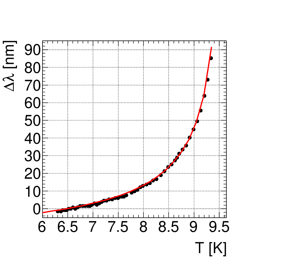
Figure 2 and 2 show typical measurement data. The solid lines shown on the data points are the results of the fitting reported in this study. Special care was taken in order to eliminate non-BCS-MB phenomena. First, $E_{\rm acc}$ was kept at a low field (accelerating field of $0.3$ MV/m or peak magnetic field of $3$ mT) to avoid the systematic errors caused by the Q-slope problem [16]. Also, the measurement was done after a thermal cycle during which the cavity was cooled as slowly as possible in order to achieve a uniform temperature distribution on the surface [17].

The fitting procedure was as follows. First, $R_{\rm res}$ was removed by fitting the empirical formula shown in (2). The BCS-MB term of the data was then defined as

Second, the critical temperature $T_{\rm c}$ was determined by a Meissner effect measurement using the flux-gate sensors around the cavity. Third, the starting temperature of the frequency measurement $T_{0}$ was fixed. Finally, the temperature dependent surface resistance $R_{\rm data}$ and shift in effective penetration depth $\Delta\lambda$ were fitted by the numerical calculation of BCS theory to determine remaining four free material parameters $\left(\xi_{0},\lambda_{L},l,\Delta_{0}/k_{\rm B}T_{\rm c}\right)$. The fitting could be done by minimizing $\chi^{2}$ defined by

where $n_{R_{\rm s}}$ and $n_{\lambda}$ are the number of data points of surface resistance and penetration depth measurement, respectively, and $\sigma_{R_{\rm s}}(j)$ and $\sigma_{\lambda}(j)$ are their associated standard deviations at point $j$ ⁴⁴endnote: ⁴ These standard deviations contain systematic uncertainties commonly shared by all the data points, as well as fluctuations of the data do not necessarily follow Gaussian distributions. Therefore, the $\chi^{2}$ defined here does not necessarily obey the proper $\chi^{2}$ distribution, and confidence intervals may not be well defined. However, the minimum of the $\chi^{2}$ can still reliably determine the best fitting parameters.. There are two sets of parameters, one which gives the minimum $\chi^{2}(R_{\rm s})$ and one which gives the minimum $\chi^{2}(\lambda)$. These two results should be consistent and should be averaged, or should converge into one solution after some iterations.

However, the strategy described above did not work well. The strong correlations which exist between estimators for the fitting parameters $\left(\xi_{0},\lambda_{L},l,\Delta_{0}/k_{\rm B}T_{\rm c}\right)$ prevented a non-linear minimizer from finding the solution. In order to see this effect, a grid search was done using Linux cluster. A job for a single CPU was coded as

• •

  $l$ scan: $80$ points between $25$ nm and $185$ nm

• •

  $\Delta_{0}/k_{\rm B}T_{\rm c}$ scan: $10$ points between $1.5$ and $2.5$

• •

  $\chi^{2}$ calculation for $n_{R_{\rm s}}\sim 80$ and $n_{\lambda}\sim 50$.

This single job took several hours by Intel Core Processor i7 (Haswell, no TSX). The jobs were distributed to 700 CPUs by

• •

  $\xi_{0}$ scan: $35$ points between $10$ nm and $45$ nm

• •

  $\lambda_{\rm L}$ scan: $20$ points between $20$ nm and $40$ nm

A typical result of the $\chi^{2}$ distribution for the surface resistance is shown in Fig. 3. Note that this is only a two dimensional cross-section of a four dimensional hyper-surface of the input parameters. There is a valley of minimum $\chi^{2}$ and therefore the standard minimizer calculating partial differentials of $\chi^{2}$ by the parameters got lost. This is a demonstration of the strong correlations among estimators of parameters ⁵⁵endnote: ⁵ As a sanity check, a dummy data set produced by the BCS code itself was fitted by the same code. The $\chi^{2}$ converges to zero with the true parameters, but the region of minimum is very narrow and immediately smeared by finite experimental fluctuations. . In this example, the correlation between $\lambda_{\rm L}$ and $\xi_{0}$ values indicates that a curve of the function $R_{\rm BCS}$ modified by higher $\lambda_{\rm L}$ can be recovered by higher $\xi_{0}$, and they are thus uncertain. In other words, it is easily possible that the best fitted parameters from the surface resistance are far from those independently determined by the penetration depth.

As another group reported [18], combining surface resistance and penetration depth can mitigate the correlations. Figure 4 shows the $\chi^{2}$ distribution obtained by the penetration depth measurement. As the function of $\lambda_{\rm BCS}$ depends on $(\xi_{0},\lambda_{\rm L})$ differently from that of $R_{\rm BCS}$, the valley of minimum $\chi^{2}$ has an intersection with Fig. 3 near the center of the plot. Such an intersection may be a robust guess of the true solution in this two dimensional surface.

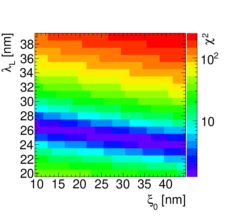
In order to obtain the intersection, we considered the sum of the two independent $\chi^{2}$s⁶⁶endnote: ⁶ The normalization by the minimum $\chi^{2}$ enforces the same weight or significance to the two different data. In this analysis, the statistical and systematic errors in the data are overwhelmed by the uncertainty due to the structure of the parameter correlations. The $\chi^{2}$ variation around the global minimum of this modified $\chi^{2}$ may not give the statistically well defined confidence intervals. However, this $\chi^{2}$ still provides a reasonable indicator of the uncertainty of the parameters associated with the correlations.

The result is shown in Fig. 5. The problematic valley of the $\chi^{2}$ minimum becomes smaller, where two parameters $(\xi_{0},\lambda_{\rm L})$ were more precisely confined. This simultaneous fit worked well for most of the sets of parameters: $(\xi_{0},\lambda_{\rm L})$, $(\lambda_{\rm L},l)$, $(\xi_{0},\Delta_{0}/k_{\rm B}T_{\rm c})$, $(\lambda_{\rm L},\Delta_{0}/k_{\rm B}T_{\rm c})$, and $(l,\Delta_{0}/k_{\rm B}T_{\rm c})$.

However, the correlation of $(\xi_{0},l)$ cannot be solved by this method as shown in Fig. 6. This is because both the surface resistance and the penetration depth depend on $(\xi_{0},l)$ similarly. The well confined result of $(\xi_{0},\lambda_{\rm L})$ and others is just one of the cross-sections of this remaining valley, and not the true solution.

In previous studies on bulk Nb, Nb₃Sn and N-doped bulk Nb [18], this correlation was eliminated by using literature values for $(\xi_{0},\lambda_{\rm L})$. For a clean bulk Nb cavity, this assumption is reasonable ($\xi_{0}=39$ nm and $\lambda_{L}=32$ nm [19]). However, for the sputtered film cavity, the literature value may not be accurate because the material has a very fine structure of grain boundaries and many dislocations. In this study, we aimed to avoid using any literature values and just used the experimental data and BCS theory. Apparently, RF surface resistance and penetration depth measurement were not sufficient for this purpose.

A series of magnetization measurements of one sample was carried out using SQUID-VSM. Figure 7 shows a typical result at 4.5 K. The lower critical field ($B_{\rm c1}$) is strongly affected by the demagnetization factor, and could not be determined precisely by this method. The upper critical field $B_{\rm c2}$ is a more robust observable and can be determined relatively precisely as the x-intersect of Fig. 7.

The temperature dependence of $B_{\rm c2}$ was measured as shown in Fig. 8. In the dirty limit, a full numerical calculation developed by using BCS-Gor’kov formalism [20] can be well approximated by an empirical formula [21]

where $C_{1}=0.153$, $C_{2}=0.152$ are fixed, and $B_{\rm c2}(0)$ is the only free parameter. The number $0.693$ changes to $0.72$ in the clean limit; thus, the uncertainty by ignoring the mean free path is less than $5$%. The solid line shown in Fig. 8 is the best fit of (10).

The dashed line in Fig. 8 shows the Ginzburg-Landau theory tangentially fitted at $T\rightarrow T_{\rm c}$

where $\Phi_{0}$ is the flux quantum, and $\xi_{\rm GL}$ is the Ginzburg-Landau coherence length

Note that (11) and (12) are only valid near $T_{\rm c}$. Therefore, the dashed line over-estimates $B_{\rm c2}$ at $T=0$ by about $30$% as shown in Fig. 8.

Since expansion of BCS-Gor’kov theory near $T_{\rm c}$ reproduces the Ginzburg-Landau theory [22], the relation between BCS material parameters $(\xi_{0},l)$ and $\xi_{\rm GL}(T)$ is obtained by this expansion for arbitrary impurity [23]

where $1=R(0)<R(l)<R(\infty)=1.17$. Once the material parameters $(\xi_{0},l)$ are provided, (13), (11) and (10) lead to a theoretical estimation of $B_{\rm c2}(0)$. One must not forget the factor $\sim 0.7$ to translate Ginzburg-Landau theory near $T_{\rm c}$ to BCS theory at $T=0$.

These formulae can be used as another constraint to the BCS parameters. Using (11) and (13), we obtain

where $t=T/T_{\rm c}$. The slope was given by the linear fitting by the dashed line in Fig. 8, and provided a relation between possible $\xi_{0}$ and $l$ values.

This constraint between two BCS parameters $\xi_{0}$ and $l$ is complementary to the surface impedance measurement. The solid line on Fig. 6 shows this additional constraint, and the star is the minimum $\chi^{2}$ satisfying the condition given by the magnetometry. This method got rid of the last correlation among the parameters and the material parameters were uniquely determined based on experimental data and BCS theory.

References

- [1] Y. Kadi, et al., J. Phys. G 44, 084003 (2017).
- [2] M. Borge and Y. Kadi, “ISOLDE at CERN”, Nuclear Physics News 26, 4 (2016).
- [3] I. Ben-Zvi and J. M. Brennan, Nucl. Instrum. Meth. 212, 73 (1983).
- [4] A. Sublet, et al., “Niobium coated HIE-ISOLDE QWR superconducting accelerating cavities coating process and film characterization”, in 6th International Workshop on Thin Films, INFN-LNL Legnaro, Italy, October 6–8, 2014.
- [5] J. Bardeen, L. N. Cooper, and J. R. Schrieffer, Phys. Rev. 108, 1175 (1957).
- [6] D. C. Mattis and J. Bardeen, Phys. Rev. 111, 412 (1958).
- [7] A. A. Abrikosov, L. P. Gor’kov, I. M. Khalatnikov, JTEP, 8, 1, 182 (1959).
- [8] J. Halbritter, Z. Physik 238, 466 (1970).
- [9] J. Halbritter, “– A FORTRAN-program for the computation of Surface Impedance of Superconductors”, Externer Beficht 3/70-6 (Kernforschtmgszentrum Karlsruhe, 1970)
- [10] G. E. H. Reuter and E. H. Sondheimer, Proc. Roy. Soc. A 195, 336 (1948).
- [11] https://www.cst.com/products/cstmws
- [12] http://www.ansys.com/products/electronics/ansys-hfss
- [13] J. Halbritter, Z. Physik 266, 209 (1974)
- [14] T. Kubo and A. V. Gurevich,“ A unified theory of surface resistance and the residual resistance of SRF cavities at low temperatures”, 18th International Conference on RF Superconductivity, Lanzhou, China, July 17–21, 2017.
- [15] T. Junginger, “Investigation of the surface resistance of superconducting materials”, Ph.D. thesis (Heidelberg University, 2012);
- [16] C. Benvenuti, et al., Physica C 316, 153 (1999).
- [17] P. Zhang, et al.. “The influence of cooldown conditions at transition temperature on the quality factor of niobium sputtered quater-wave resonantors for HIE-ISOLDE ”, 17th International Conference on RF Superconductivity, Whistler, Canada, September 13–18, 2015.
- [18] N. R. A. Valles, “Pushing the frontiers of superconducting radio frequency science: From the temperature dependence of the superheating field of niobium to higher-order mode damping in very high quality factor accelerating structures”, Ph.D. thesis (Cornell University, 2014); S. E. Posen, “Understanding and overcoming limitation mechanisms in Nb3Sn superconducting RF cavities”, Ph.D. thesis (Cornell University, 2015); D. Gonnella, “The fundamental science of nitrogen-doping of niobium superconducting cavities”, Ph.D. thesis (Cornell University, 2016)
- [19] J. P. Turneaure, et at., J. Supercond. 4, 341 (1991).
- [20] E. Helfand and N. R. Werthamer, Phys. Rev. 147, 288 (1966).
- [21] T. Baumgartner, “Effects of fast neutron irradiation on critical currents and intrinsic properties of state-of-the-art Nb3Sn wires”, PhD thesis (Vienna University of Technology, 2013).
- [22] L. P. Gor’kov, JTEP, 9, 1364 (1959).
- [23] T. P. Orlando, et al., Phy. Rev. B 19, 4545 (1979).
- [24] T. Junginger, et al., accepted by Supercond. Sci. Technol. (https://doi.org/10.1088/1361-6668/aa8926).
- [25] J. Halbritter, Z. Physik 243, 201 (1971).
- [26] B. B. Goodman and G. Kuhn, J. Phys. France 29, 240-252 (1968)
- [27] D. Bloess, et at., “Superconducting, hydroformed, niobium sputter coated cavities at 1.5 GHz”, Proc. EPAC London 27 June – 1 July 1995,
- [28] W. Weingarten, “Progress in Thin Film Techniques”, Proc. 7th Workshop on RF Superconductivity, Gif-sur-Yvette, France, October, 1995.
- [29] H. Padamsee, et al., “RF Superconductivity for Accelerators”, Wiley, Weinheim, second edition, 2008.