On the turnpike phenomenon for optimal boundary control problems with hyperbolic systems

Martin Gugat Falk M. Hante ^†^†thanks: Friedrich–Alexander–Universität Erlangen–Nürnberg, Department Mathematik, Cauerstr.˜11, 91058 Erlangen, Germany (martin.gugat@fau.de, falk.hante@fau.de)

August 24, 2026

Abstract: We study problems of optimal boundary control with systems governed by linear hyperbolic partial differential equations. The objective function is quadratic and given by an integral over the finite time interval $(0,\,T)$ that depends on the boundary traces of the solution. If the time horizon $T$ is sufficiently large, the solution of the dynamic optimal boundary control problem can be approximated by the solution of a steady state optimization problem. We show that for $T\rightarrow\infty$ the approximation error converges to zero in the sense of the norm in $L^{2}(0,\,1)$ with the rate $1/T$ , if the time interval $(0,\,T)$ is transformed to the fixed interval $(0,\,1)$ . Moreover, we show that also for optimal boundary control problems with integer constraints for the controls the turnpike phenomenon occurs. In this case the steady state optimization problem also has the integer constraints. If $T$ is sufficiently large, the integer part of each solution of the dynamic optimal boundary control problem with integer constraints is equal to the integer part of a solution of the static problem. A numerical verification is given for a control problem in gas pipeline operations.

Keywords: Hyperbolic system, boundary control, optimal control, turnpike, integer constraints

AMS: 35L04, 49K20, 90C46

0.1 Introduction

Boundary control problems for systems governed by hyperbolic partial differential equations (pdes) appear in many applications, for example water or gas transportation systems, see e.g. [3]. Applications of this type give rise to optimal boundary control problems, where an objective function models the aims of the control design. In these control problems, it makes sense to consider finite time horizons. An overview of the quadratic optimal control of hyperbolic partial differential equations is given in [24]. In this paper we are interested in results about the structure of the optimal boundary controls in the spirit of the turnpike theory. Since the evolution of the state in time is governed by the hyperbolic pde, we call the corresponding optimal controls the dynamic optimal controls. The turnpike phenomenon can be summarized in the statement that in large time intervals, the optimal state, control and adjoint vector remain most of the time close to an optimal steady-state (see [29]). This means that in order to get an idea of the dynamic optimal controls, it make sense to look at the solution of a certain static boundary control problem first, where all time derivatives are set to zero. This static control problem determines optimal static states. Let us call the corresponding optimal control the static optimal control. Our aim is to give a bound for the difference between the static optimal control (that is independent of time) and the dynamic optimal control.

Turnpike theory has originally been discussed in economics, see [8]. Turnpike properties for discrete–time optimal control problems have been studied in [7], [11]. Recently there has been some interest in the study of the turnpike phenomenon for infinite dimensional optimal control problems, in particular with systems governed by pdes, see for example [26] for the linear case, [27] for the parabolic semilinear case and [31] for optimal shape design with the heat equation. Problems with infinite-dimensional control systems have also been studied in [33]. The results can be applied to control systems with distributed control. In this paper, we consider boundary control systems that are governed by hyperbolic pdes. Optimal Neumann boundary control problems for systems governed by the wave equation have been studied in [15]. A review of turnpike results for wave equations is given in [35].

In [7], [11] and the recent contributions [9], [30] on turnpike theory, dissipativity plays an essential role. In [9], system states in a finite-dimensional space are considered. In [30] infinite-dimensional states spaces are considered and the control acts as a distributed control in the partial differential equation in such a way that mild solutions are well-defined. In [30], both integral- and measure–turnpike properties are considered. In this paper, we consider integral–turnpike properties. Here we mention that the optimal control problems that we consider in this paper (i.e. (7), (15)) satisfy a dissipation inequality as defined in [30] if there exists a number $\Xi_{0}>0$ such that the supply rate function $\omega(u)$ as a function of the control $u$ satisfies the inequality $\int_{0}^{t}\omega(u(\tau))\,d\tau\geq\Xi_{0}\|u\|_{(L^{2}(0,\,t))^{2}}^{2}$ . Then we can find a number $\Xi_{1}>0$ such that for a state $r\in(L^{2}(0,L))^{2}$ the storage function $S(r)=\Xi_{1}\,\|r\|_{(L^{2}(0,L))^{2}}^{2}$ satisfies a dissipation inequality.

In this paper we study optimal Dirichlet boundary control problems for systems that are governed by linear $2\times 2$ hyperbolic pdes. A similar problem of optimal boundary control is studied in [20], but the turnpike phenomenon is not considered. Our motivation for this setting is to obtain structural insights for the optimal control of gas flow in pipelines. Also the linearized Saint-Venant equations, that can be used as a model for the flow of water through channels, have this form, see [4]. In these applications, also binary decisions are important to model for example the decision to open or close a certain valve or to switch on or off a control device such as a compressor [18]. This motivates the study of optimal boundary control problems with integer constraints.

This paper has the following structure. In Section 0.2 we define the system dynamics and present our results for optimal boundary control problems for unconstrained and integer-constrained cases. In Section 0.3 a proof is given for the main result concerning the unconstrained case. In Section 0.4 we prove our result for the integer-constrained case. In Section 0.5 we discuss an application of our results to optimized operation of gas pipelines and provide a numerical verification. In Section 0.6 we present conclusions.

0.2 Problem definition and main results

0.2.1 Hyperbolic system dynamics

The aim of this contribution is to study the turnpike phenomenon for systems that are governed by hyperbolic pdes. We consider a $2\times 2$ system in diagonal form. Let a length $L>0$ and a time interval $[0,T]$ be given. Let $d_{-}$ and $d_{+}$ be real-valued continuously differentiable functions that are defined on the space-interval $[0,\,L]$ such that for all $x\in[0,\,L]$ the inequality $d_{-}(x)<0<d_{+}(x)$ holds. Define the ( $x$ -dependent) diagonal matrices

D(x)=\left(\begin{array}[]{cc}d_{+}(x)&0\\ 0&d_{-}(x)\end{array}\right),\;\;D^{\prime}(x)=\left(\begin{array}[]{cc}d_{+}^{\prime}(x)&0\\ 0&d_{-}^{\prime}(x)\end{array}\right).

For all $x\in[0,\,L]$ , let $M(x)$ denote a $2\times 2$ matrix that depends continuously on $x$ . Let $\eta_{0}\leq 0$ be a real number. For real numbers $\mu_{+}$ , $\mu_{-}$ define the matrix

E(x)=\left(\begin{array}[]{cc}\exp(-\mu_{+}\,x)&0\\ 0&\exp(\mu_{-}\,\,x)\end{array}\right).

(1)

Assume that there exist $\mu_{+}>0$ , $\mu_{-}>0$ and $\nu_{a}<0$ such that for all $x\in[0,\,L]$

\sup_{v:\,v^{\top}E(x)\,v=1}v^{\top}\left[\frac{d}{dx}\left(E(x)D(x)\right)-|\eta_{0}|\left(E(x)M(x)+M(x)^{\top}E(x)\right)\right]v\leq\nu_{a}.

(2)

Moreover, assume that there exist $\mu_{+}<0$ , $\mu_{-}<0$ and $\nu_{0}>0$ such that for all $x\in[0,\,L]$

\inf_{v:\,v^{\top}E(x)\,v=1}v^{\top}\left[E^{\prime}(x)D(x)-E(x)D^{\prime}(x)+|\eta_{0}|\left(E(x)M(x)+M(x)^{\top}E(x)\right)\right]v\geq\nu_{0}.

(3)

Remark 1

If $M(x)$ is a diagonal matrix or if $|\eta_{0}|$ is sufficiently small or if $L>0$ is sufficiently small, (2) and (3) hold. If $M^{\top}=M$ , (2) and (3) are equivalent with $\nu_{0}=-\nu_{a}$ .

Consider the linear hyperbolic pde

r_{t}+D\,r_{x}=\eta_{0}\,M\,r

(4)

where for $x\in(0,\,L)$ and $t\in(0,T)$ , the state is given by $r(t,\,x)=\left(\begin{array}[]{r}r_{+}(t,\,x)\\ r_{-}(t,\,x)\end{array}\right).$ To obtain an initial boundary value problem, in addition to (4) we consider the initial condition $r(0,\,x)=0$ for $x\in(0,\,L)$ at the time $t=0$ and for $t\in(0,T)$ the Dirichlet boundary conditions $r_{+}(t,\,0)=u_{+}(t),\;r_{-}(t,\,L)=u_{-}(t)$ with boundary controls $u_{+}$ , and $u_{-}$ in $L^{2}(0,T)$ . The resulting initial boundary value problem

\left\{\begin{array}[]{l}r(0,\,x)=0,\\ r_{t}+D\,r_{x}=\eta_{0}\,M\,r,\\ r_{+}(t,\,0)=u_{+}(t),\\ r_{-}(t,\,L)=u_{-}(t),\end{array}\right.

(5)

has a solution $r\in C([0,T],L^{2}((0,\,L);{\mathbb{R}}^{2}))$ . Moreover, for the boundary traces of the solution we have $r_{+}(\cdot,L)$ , $r_{-}(\cdot,\,0)\in L^{2}(0,\,T)$ . This follows with a Picard iteration along the characteristic curves similar as in [21], [22].

0.2.2 Unconstrained optimal boundary control

In this section we define a dynamic optimal boundary control problem for (4) along with a corresponding static optimal control problem and state the result relating the solutions of the two problems.

For $x=(x_{+},\,x_{-})^{\top}\in{\mathbb{R}}^{2}$ , we use the notation $\|x\|_{{\mathbb{R}}^{2}}=\left|x_{+}^{2}+x_{-}^{2}\right|^{1/2}$ . Let strictly convex quadratic functions $f_{0}$ and $f_{L}$ be given, that is for $z\in{\mathbb{R}}^{2}$ we have $f_{0}(z)=\tfrac{1}{2}z^{\top}A_{0}z+c_{0}^{\top}z$ , $f_{L}(z)=\tfrac{1}{2}z^{\top}A_{L}z+c_{L}^{\top}z$ , with symmetric positive definite $2\times 2$ matrices $A_{0}$ , $A_{L}$ and vectors $c_{0}$ , $c_{L}\in{\mathbb{R}}^{2}$ . Define the Hilbert space $H=L^{2}(0,\,T)\times L^{2}(0,\,T).$ For $u=(u_{+},u_{-})\in H$ and $R=(R_{+},R_{-})\in H$ , define

J(u,\,R)=\int_{0}^{T}f_{0}(u_{+}(t),\,R_{-}(t))+f_{L}(u_{-}(t),\,R_{+}(t))\,dt.

(6)

Remark 2

The assumption of strict convexity of $f_{0}$ and $f_{L}$ can be slightly relaxed. Only the strict convexity with respect to the control is essential. Our results also hold if for $q$ as defined in (56) there exists a constant $\kappa>0$ such that (60) holds.

The choice of the objective function $J(u,\,R)$ is motivated by transportation systems such as gas pipelines, see Section 0.5. We consider the dynamic optimal control problem

\left\{\begin{array}[]{l}\min_{u\in(L^{2}(0,\,T))^{2}}J(u,\,(r_{+}(\cdot,L),\,r_{-}(\cdot,\,0)))\\ \mbox{\rm subject to (\ref{linearizedsystem})}.\end{array}\right.

(7)

With a slight abuse of notation, in the sequel we write $J(u,\,r)$ instead of

J(u,\,(r_{+}(\cdot,L),\,r_{-}(\cdot,\,0))).

Our assumptions imply that the objective function grows as fast as some real constant multiplied with $\|u_{+}\|_{L^{2}(0,\,T)}^{2}+\|u_{-}\|_{L^{2}(0,\,T)}^{2}$ . Hence the existence of an optimal control follows with the Direct Method of the Calculus of Variations by considering a minimizing sequence and going to a weakly converging subsequence.

In the corresponding static optimal control problem the initial boundary value problem (5) is replaced by the boundary value problem

\left\{\begin{array}[]{l}D\,R^{(\upsigma)}_{x}(x)=\eta_{0}\,M\,R^{(\upsigma)}(x),\\ R_{+}^{(\upsigma)}(0)=u_{+}^{(\upsigma)},\\ R_{-}^{(\upsigma)}(L)=u_{-}^{(\upsigma)},\end{array}\right.

(8)

with $x\in(0,\,L)$ and $u^{(\upsigma)}=\left(u_{+}^{(\upsigma)},\,u_{-}^{(\upsigma)}\right)^{\top}\in\mathbb{R}^{2}$ . Define the objective function

J_{0}(u^{(\upsigma)},\,R^{(\upsigma)}(x))=f_{0}(u^{(\upsigma)}_{+},\,R_{-}^{(\upsigma)}(0))+f_{L}(u^{(\upsigma)}_{-},\,R_{+}^{(\upsigma)}(L)).

(9)

The static optimization problem that corresponds to the dynamic problem (7) is

\left\{\begin{array}[]{l}\min_{u^{(\upsigma)}\in\mathbb{R}^{2}}J_{0}(u^{(\upsigma)},\,R^{(\upsigma)}(x))\\ \mbox{\rm subject to (\ref{staticlinearizedsystem})}.\end{array}\right.

(10)

We show in Section 0.3 that solutions of the dynamic and static problem are related in the sense of the following turnpike result.

Theorem 1

Let $u^{(\upsigma)}$ denote the optimal static control that solves (10) and let $u^{(\updelta,\,T)}$ denote the optimal dynamic control that solves (7) with the finite time horizon $T>0$ . Let $r^{(\upsigma)}$ and $r^{(\updelta,\,T)}$ denote the corresponding states. There exists a constant $\bar{C}>0$ that is independent of $T$ such that for all $T>0$

\frac{1}{T}\,\int_{0}^{T}\left\|u^{(\updelta,\,T)}(\tau)-u^{(\upsigma)}\right\|^{2}_{{\mathbb{R}}^{2}}\,d\tau\leq\frac{\bar{C}}{T}.

(11)

Thus for all $T>0$ we have the inequality $\int_{0}^{1}\left\|u^{(\updelta,\,T)}(T\,s)-u^{(\upsigma)}\right\|^{2}_{{\mathbb{R}}^{2}}\,ds\leq\frac{\bar{C}}{T}.$ Moreover, there exists a constant $\tilde{D}>0$ such that for all $T>0$ we have

\int_{0}^{T}\int_{0}^{L}\left\|r^{(\updelta,\,T)}(\tau,\,x)-r^{(\upsigma)}(x)\right\|^{2}_{\mathbb{R}^{2}}\,d\tau\leq\tilde{D}.

(12)

Theorem 1 states that for increasing time horizon $T\rightarrow\infty$ , the average quadratic mean distance between the optimal dynamic and the optimal static control converges to zero with the rate $O(\frac{1}{T})$ .

Example 1

Let real numbers $R_{+}^{\flat}$ , $R_{-}^{\flat}$ and $\lambda\in(0,\,1)$ be given. Consider

J(u,\,R)=\int_{0}^{T}(1-\lambda)\,\left\|\left(\begin{array}[]{l}R_{+}(t)-R_{+}^{\flat}\\ R_{-}(t)-R_{-}^{\flat}\end{array}\right)\right\|^{2}_{{\mathbb{R}}^{2}}+\lambda\,\left\|\left(\begin{array}[]{l}u_{+}(t)\\ u_{-}(t)\end{array}\right)\right\|^{2}_{{\mathbb{R}}^{2}}\,dt.

(13)

The objective function $J(u,\,r)$ is of the form (6) up to additive constants. Since the system is hyperbolic, there exists times $t_{+}$ , $t_{-}\in(0,\,T)$ , such that for $t>t_{\pm}$ , the control value $u_{\pm}(t)$ does not influence the state $r_{+}(\cdot,L)$ , $r_{-}(\cdot,0)$ respectively. Thus definition (13) implies that for $t>t_{\pm}(t)$ , we have $u^{(\updelta,\,T)}_{\pm}(t)=0$ that is in the last part of the time interval the control is switched off since we did not impose any condition on the terminal state $r_{\pm}(T,\,\cdot)$ (in contrast to [15]). If $D$ and $M$ are constant diagonal matrices, we have $u_{\pm}^{(\updelta,\,T)}(t)=0$ for $t>t_{\pm}=T-L/|d_{\pm}|$ and $u^{(\upsigma)}_{\pm}=\left[\frac{1}{\tfrac{1}{\lambda}-1}+\exp\left(\eta_{0}\tfrac{m_{\pm\pm}}{|d_{\pm}|}\,L\right)\right]^{-1}R_{\pm}^{\flat}$ . Moreover, for $t<t_{\pm}$ we have $u_{\pm}^{(\updelta,\,T)}(t)=u^{(\upsigma)}_{\pm}$ . Hence $\int_{0}^{T}\left\|u^{(\updelta,\,T)}(\tau)-u^{(\upsigma)}\right\|^{2}_{{\mathbb{R}}^{2}}\,d\tau=\tfrac{L}{d_{+}}\,|u^{(\upsigma)}_{+}|^{2}+\tfrac{L}{|d_{-}|}\,|u^{(\upsigma)}_{-}|^{2}.$

0.2.3 Optimal boundary control problems with an integer control constraint

In the application often controls with a finite range of control values appear. In particular, binary decisions can be modeled in this form. For overviews on optimal control problems of this type see [34], [17] and the references therein. In this section we show that also for these problems, the turnpike phenomenon can occur. Let ${\cal F}$ denote a finite set of integers that contains zero. We consider the integer constraint

u_{+}(t)\in{\color[rgb]{0,0,0}\cal F}\;\;\;\mbox{\rm for $t$ almost everywhere in $(0,T)$.}

(14)

The controls that satisfy (14) are simple functions with values in ${\color[rgb]{0,0,0}\cal F}$ almost everywhere. In order to avoid chattering controls that switch infinitely often between the values in ${\color[rgb]{0,0,0}\cal F}$ (this is also called the Zeno phenomenon), in the objective function switching costs are added that penalize the switching. For this purpose we use a penalty term with the total variation

{\rm Var}(u_{+})=\int_{0}^{T}d\left|u_{+}\,\right|=\sup\limits_{P}\sum_{i}\left|u_{+}(t_{i+1})-u_{+}(t_{i})\right|,

where the supremum is over all possible finite partitions $P$ of $[0,\,T]$ .

In order to make the discussion more concise, we assume for the integer constrained case that $J$ is as in (13). Let a penalty parameter $\nu>0$ be given. Consider the dynamic optimal boundary control problem with integer control constraint

\left\{\begin{array}[]{l}\min_{u\in(L^{2}(0,\,T))^{2}}J(u,\,r)+\nu\,T\,{\rm Var}(u_{+})\\ \mbox{\rm subject to $(u,\,r)$ solves (\ref{linearizedsystem})}\,\;{\mbox{\rm and $u_{+}$ satisfies}}\;\;(\ref{21122016}).\end{array}\right.

(15)

The additional switching–cost term in the objective functions penalizes the number of switchings between the values in ${\color[rgb]{0,0,0}\cal F}$ . Existence of optimal solutions then follows from a compactness argument similar as in [19]. Let $\omega(T)$ denote the optimal value of the dynamic optimal control problem (15). The corresponding static optimal control problem with integer constraint is

\left\{\begin{array}[]{l}\min_{u^{(\upsigma)}_{+}\in{\color[rgb]{0,0,0}\cal F},\,u^{(\upsigma)}_{-}\in{\mathbb{R}},\,\,R^{(\upsigma)}\in(L^{2}(0,\,L))^{2}}J_{0}(u^{(\upsigma)},\,R^{(\upsigma)})\\ \mbox{\rm subject to (\ref{staticlinearizedsystem}) }\end{array}\right.

(16)

with $J_{0}(u^{(\upsigma)},\,R^{(\upsigma)})=(1-\lambda)\,\left\|R^{(\upsigma)}-R^{\flat}\right\|^{2}_{{\mathbb{R}}^{2}}+\lambda\,\left\|u^{(\upsigma)}\right\|^{2}_{{\mathbb{R}}^{2}}$ . In the objective function of the static problem (16), the switching cost does not appear. If we insert the zero control $(u_{+}(t),\,u_{-}(t))=(0,0)$ in the objective function, the switching constraint (14) is satisfied and we also obtain an upper bound for the optimal value $\omega(T)$ . Since the zero control generates the zero state, we have $\omega(T)\leq(1-\lambda)\,T\,\|R^{\flat}\|^{2}_{\mathbb{R}^{2}}$ . For the optimal dynamic control $u^{(\ast)}$ that solves (15) this yields ${\rm Var}(u_{+}^{(\ast)})\leq\frac{1}{\nu}\,(1-\lambda)\,\|R^{\flat}\|^{2}_{\mathbb{R}^{2}}$ . Hence if

\nu>(1-\lambda)\,\|R^{\flat}\|^{2}_{\mathbb{R}^{2}}

(17)

the optimal control $u_{+}^{(\ast)}$ at $x=0$ is constant. In this case $\omega(T)$ is equal to the optimal value of the problem

\left\{\begin{array}[]{l}\min_{u_{+}\in{\color[rgb]{0,0,0}\cal F},\,u_{-}\in L^{2}(0,\,T)}J(u,\,r)\\ \mbox{\rm subject to $(u,\,r)$ solves (\ref{linearizedsystem})}.\end{array}\right.

(18)

If a given value of $u_{+}\in{\color[rgb]{0,0,0}\cal F}$ is fixed in (18), we obtain an optimal boundary control problem with a time–dependent control $u_{-}(t)$ at $x=L$ and constant boundary control at $x=0$ . The turnpike results from Section 0.2.2 can be adapted to this situation.

In Theorem 2 we state that for sufficiently large values of $\nu$ , that is if (17) holds, the solution of (15) and the solution of the corresponding static problem (16) are related by the turnpike phenomenon.

Theorem 2

Assume that $\nu$ is sufficiently large in the sense that (17) holds. Let $u^{(\updelta,\,T)}\in(L^{2}(0,\,T))^{2}$ denote a solution of the optimal dynamic control problem (15).

There exists a constant $\bar{C}>0$ that is independent of $T$ such that for $T>0$ sufficiently large, there exists a solution $u^{(\upsigma)}$ of the optimal static control problem (16) with $u^{(\updelta,\,T)}_{+}(t)=u^{(\upsigma)}_{+}$ for all $t\in[0,\,T]$ and

\frac{1}{T}\,\int_{0}^{T}\left\|u^{(\updelta,\,T)}(t)-u^{(\upsigma)}\right\|^{2}_{{\mathbb{R}}^{2}}\,d\,t\leq\frac{\bar{C}}{T}.

(19)

Moreover, for the corresponding optimal states (12) holds.

Due to the integer constraint in general the solutions of (15) and (16) are not uniquely determined. Theorem 2 implies that if the solution of the static optimal control problem (16) is unique, for all sufficiently large time horizons $T>0$ , the first component of the dynamic optimal control is independent of $t$ and $T$ . The proof of Theorem 2 is presented in Section 0.4.

0.3 Analysis for the unconstrained case

0.3.1 An adjoint operator

For a given time $T>0$ , we define the operator $F_{T}\,(u)$ that maps the boundary control $u=(u_{+}(\cdot),\,u_{-}(\cdot))\in H$ to the boundary trace $(r_{+}(\cdot,L),\,r_{-}(\cdot,\,0))$ of the solution of the linear initial boundary value problem (5). Thus we have $F_{T}\,u=\left(\begin{array}[]{r}r_{+}(\cdot,L)\\ r_{-}(\cdot,\,0)\end{array}\right).$

For a given time $T>0$ and a given initial state $h_{0}\in(L^{2}(0,\,L))^{2}$ we define the operator $G_{T}\,(u,\,h_{0})$ that maps the boundary control $u=(u_{+},\,u_{-})\in H$ and $h_{0}$ to the solution $(r_{+},\,r_{-})\in(L^{2}((0,\,T)\times(0,\,L)))^{2}$ of the initial boundary value problem

\left\{\begin{array}[]{l}r(0,\,x)=h_{0}(x),\\ r_{t}+D\,r_{x}=\eta_{0}\,M\,r,\\ r_{+}(t,\,0)=u_{+}(t),\\ r_{-}(t,\,L)=u_{-}(t).\end{array}\right.

(20)

Lemma 1

Let $u\in H$ be given. There exists a constant $\tilde{C}>0$ that is independent of $T$ such that for all $T>0$ we have

\int_{0}^{T}\int_{0}^{L}\left\|(G_{T}(u,\,h_{0}))(\tau,\,x)\right\|^{2}_{\mathbb{R}^{2}}\,dx\,d\tau\leq\tilde{C}\left(\left\|u\right\|^{2}_{H}+\left\|h_{0}\right\|^{2}_{(L^{2}(0,\,L))^{2}}\right).

(21)

Proof 1

Let real numbers $\mu_{+}>0$ and $\mu_{-}>0$ be given. Define the matrix $E(x)$ as in (1). For $t>T$ we define $u_{\pm}(t)=0$ . For $t>0$ consider the Lyapunov functional

E_{a}(t)=\frac{1}{2}\int_{t}^{t+1}\int_{0}^{L}\left(r(\tau,\,x)\right)^{\top}\,E(x)\,r(\tau,\,x)\,dx\,d\tau

(22)

where $r$ is the solution (20) for $t>0$ . For the time derivative of $E_{a}$ we obtain

	$\displaystyle E_{a}^{\prime}(t)$	$\displaystyle=$	$\displaystyle 2\int_{t}^{t+1}\int_{0}^{L}-\left(r(\tau,\,x)\right)^{\top}\,E(x)\,D(x)\,\left(r(\tau,\,x)\right)_{x}$
		$\displaystyle-$	$\displaystyle\frac{1}{2}\,\left(r(\tau,\,x)\right)^{\top}\,E(x)\,D^{\prime}(x)\,\left(r(\tau,\,x)\right)-\left(r(\tau,\,x)\right)^{\top}\,M_{1}(x)\,\left(r(\tau,\,x)\right)\,dx\,d\tau$

with the symmetric matrix $M_{1}$ defined as

M_{1}(x)=\frac{|\eta_{0}|}{2}\left[E(x)\,M(x)+M(x)^{\top}\,E(x)\right]-\frac{1}{2}\,D^{\prime}(x)\,E(x).

(23)

Integration by parts yields $E_{a}^{\prime}(t)=T_{B}+T_{R}$ with

\displaystyle T_{B}

\displaystyle:=

\displaystyle-\int_{t}^{t+1}\left(r(\tau,\,x)\right)^{\top}\,E(x)\,D(x)\,\left(r(\tau,\,x)\right)|_{x=0}^{L}d\tau

and

	$\displaystyle T_{R}$	$\displaystyle:=$	$\displaystyle\int_{t}^{t+1}\int_{0}^{L}\left(r(\tau,\,x)\right)^{\top}\,E^{\prime}(x)\,D(x)\,\left(r(\tau,\,x)\right)\,dx\,d\tau$
			$\displaystyle-2\,\int_{t}^{t+1}\int_{0}^{L}\left(r(\tau,\,x)\right)^{\top}\,M_{1}(x)\,\left(r(\tau,\,x)\right)\,dx\,d\tau.$

Define $\xi(t)=\max\left\{|d_{-}(L)|\,{\rm e}^{\mu_{-}\,L},\;d_{+}(0)\right\}\int_{t}^{t+1}\left\|\left(u_{+}(\tau),\,u_{-}(\tau)\right)\right\|_{\mathbb{R}^{2}}^{2}\,d\tau$ . Then we have $T_{B}\leq\xi(t)$ . Due to assumption (2) we can choose $\mu_{+}>0$ and $\mu_{-}>0$ such that

\displaystyle T_{R}

\displaystyle\leq

\displaystyle\nu_{a}\,E_{a}(t).

This yields

E_{a}^{\prime}(t)=T_{B}+T_{R}\leq\nu_{a}\,E_{a}(t)+\xi(t).

By Gronwall’s Lemma this implies for all $j\in\{0,1,2,3,...\}$ the inequality

0\leq E_{a}(j+1)\leq\exp(\nu_{a})\,E_{a}(j)+\int_{j}^{j+1}\xi(t)\,dt.

By induction, this implies for all $N\in\{0,\,1,\,2,\,3,...\}$

E_{a}(j+1)\leq\exp(\nu_{a}\,(j+1))\,E_{a}(0)+\sum_{k=0}^{j}\exp(\nu_{a}\,(j-k))\,\int_{k}^{k+1}\xi(t)\,dt.

Hence we obtain

\sum_{j=0}^{N}E_{a}(j)\leq\left(\sum_{j=0}^{\infty}\exp(\nu_{a}\,j)\right)\,\left(E_{a}(0)+\sum_{j=0}^{N}\int_{j}^{j+1}\xi(t)\,dt\right).

(24)

We have

\sum_{j=0}^{N}\int_{j}^{j+1}\xi(t)\,dt=\int_{0}^{N+1}\xi(t)\,dt\leq\int_{0}^{\infty}\xi(t)\,dt.

Define $\tilde{K}=\max\left\{|d_{-}(L)|\,{\rm e}^{\mu_{-}\,L},\;d_{+}(0)\right\}$ . The definition of $\xi$ implies that

\tfrac{\int_{0}^{\infty}\xi(t)\,dt}{\tilde{K}}=\int\limits_{0}^{\infty}\int\limits_{t}^{t+1}\left\|u(\tau)\right\|_{\mathbb{R}^{2}}^{2}\,d\tau\,dt=\int\limits_{0}^{T}\int\limits_{0}^{1}\left\|u(\tau+t)\right\|_{\mathbb{R}^{2}}^{2}\,d\tau\,dt\leq\int\limits_{0}^{T}\left\|u(\tau)\right\|_{\mathbb{R}^{2}}^{2}\,d\tau.

Thus we have $\int_{0}^{\infty}\xi(t)\,dt\leq\tilde{K}\,\left\|u\right\|_{H}$ . Hence (24) implies $\sum\limits_{j=0}^{\infty}E_{a}(j)<\infty$ . There exists a number $\tilde{C}_{0}$ such that

E_{a}(0)=\frac{1}{2}\int_{0}^{1}\int_{0}^{L}\left(r(\tau,\,x)\right)^{\top}\,E(x)\,r(\tau,\,x)\,dx\,d\tau\leq\tilde{C}_{0}\left(\left\|u\right\|^{2}_{H}+\left\|h_{0}\right\|^{2}_{(L^{2}(0,\,L))^{2}}\right).

We have $\sum\limits_{j=0}^{\infty}E_{a}(j)=\frac{1}{2}\int_{0}^{\infty}\int_{0}^{L}\left(r(\tau,\,x)\right)^{\top}\,E(x)\,r(\tau,\,x)\,dx\,d\tau$ . Hence (24) yields

\int\limits_{0}^{\infty}\int\limits_{0}^{L}\left(r(\tau,\,x)\right)^{\top}\,E(x)\,r(\tau,\,x)\,dx\,d\tau\leq\frac{2}{1-{\rm e}^{\nu_{a}}}\left(\tilde{C}_{0}+\tilde{K}\right)\left(\left\|u\right\|^{2}_{H}+\left\|h_{0}\right\|^{2}_{(L^{2}(0,\,L))^{2}}\right).

This implies (21).

Using Lemma 1 and integration by parts we can prove Lemma 2.

Lemma 2

The operator $F_{T}$ is uniformly bounded as an operator in the Hilbert space $H$ that is there exists a constant $C_{N}>0$ that is independent of $T$ such that for the corresponding operator norm of $F_{T}$ for all $T>0$ we have

\|F_{T}\|\leq C_{N}.

(25)

For the analysis of the boundary control problem, the study of the adjoint operators for $F_{T}$ defined at the end of 0.3.1 is essential. The adjoint operator $F_{T}^{\ast}$ that satisfies the equation

\int_{0}^{T}\left\langle F_{T}\,(u)(t),\,z_{T}(t)\right\rangle_{\mathbb{R}^{2}}\,dt=\int_{0}^{T}\left\langle u(t),\,F_{T}^{\ast}(z_{T})(t)\right\rangle_{\mathbb{R}^{2}}\,dt

(26)

for all $z_{T}\in{\cal D}(F_{T}^{\ast})=H$ where $\langle\cdot,\,\cdot\rangle_{{\mathbb{R}}^{2}}$ denotes the usual scalar product in ${\mathbb{R}}^{2}$ . Due to (25) we have the inequality

\|F_{T}^{\ast}\|\leq C_{N}.

(27)

Similar as in [6], we determine $F_{T}^{\ast}$ in the following lemma.

Lemma 3

For $z_{T}=(z_{+}^{T},\,z_{-}^{T})\in{\cal D}(F_{T}^{\ast})=H$ , define $z=(z_{+}(\cdot),\,z_{-}(\cdot))$ as the solution of the adjoint system (where $(t,\,x)\in(0,\,T)\times(0,\,L)$ )

\left\{\begin{array}[]{l}z(T,\,x)=0,\,x\in(0,L),\\ z_{t}(t,\,x)+D\,z_{x}(t,\,x)=-\eta_{0}\,M(x)^{\top}\,z(t,\,x)-D^{\prime}(x)\,z(t,\,x),\\ z_{+}(t,\,L)=\frac{1}{d_{+}(L)}\,z_{+}^{T}(t),\\ z_{-}(t,\,0)=\frac{1}{|d_{-}(0)|}\,z_{-}^{T}(t).\end{array}\right.

(28)

Then we have

F_{T}^{\ast}\,\left(\begin{array}[]{r}z_{+}^{T}(\cdot)\\ z_{-}^{T}(\cdot)\end{array}\right)=\left(\begin{array}[]{r}d_{+}(0)\,z_{+}(\cdot,\,0)\\ |d_{-}(L)|\,z_{-}(\cdot,L)\end{array}\right).

(29)

For our proof of the turnpike result, the fact that the operator norm of $F_{T}$ is uniformly bounded with respect to $T$ is essential. Moreover, it is important that with boundary controls that are zero, the system state decays exponentially with time for the forward system in the forward direction and for the adjoint system with time going backwards.

0.3.2 Necessary optimality conditions for the dynamic problem

In order to determine the structure of the dynamic optimal control $u^{(\updelta,\,T)}$ that solves (7) we look at the necessary optimality conditions. For all $u,\,r\in H$ that satisfy (5), we have

J(u,\,r)=\int_{0}^{T}f_{0}(u_{+}(t),\,(F_{T}u)_{-}(t)\,)+f_{L}(u_{-}(t),\,(F_{T}u)_{+}(t)\,)\,dt.

(30)

Let $u=u^{(\updelta,\,T)}+\delta^{(1)}$ with a control variation $\delta^{(1)}\in H$ . Let $R=R^{(\updelta,\,T)}+\delta^{(2)}$ denote the corresponding state, that is we have

\left\{\begin{array}[]{l}\delta^{(2)}(0,\,x)=0,\,x\in(0,L),\\ \delta^{(2)}_{t}+D\,\delta^{(2)}_{x}=\eta_{0}\,M\,\delta^{(2)},\\ \delta^{(2)}_{+}(t,\,0)=\delta^{(1)}_{+}(t),\\ \delta^{(2)}_{-}(t,\,L)=\delta^{(1)}_{-}(t),\end{array}\right.

or $F_{T}\,(\delta^{(1)})=\left(\delta^{(2)}_{+}(\cdot,\,L),\delta^{(2)}_{-}(\cdot,\,0)\right)^{\top}.$ Since $J$ is convex and we have

			$\displaystyle J(u^{(\updelta,\,T)}+\delta^{(1)},\,R^{(\updelta,\,T)}+\delta^{(2)})\geq J(u^{(\updelta,\,T)},\,R^{(\updelta,\,T)})$
		$\displaystyle+$	$\displaystyle\langle A_{0}\left(\begin{array}[]{c}u_{+}^{(\updelta,\,T)}\\ (F_{T}u^{(\updelta,\,T)})_{-}\end{array}\right)+c_{0},\,\left(\begin{array}[]{c}\delta^{(1)}_{+}\\ (F_{T}\delta^{(1)})_{-}\end{array}\right)\rangle_{H}+\langle A_{L}\left(\begin{array}[]{c}u_{-}^{(\updelta,\,T)}\\ (F_{T}u^{(\updelta,\,T)})_{+}\end{array}\right)+c_{L},\,\left(\begin{array}[]{c}\delta^{(1)}_{-}\\ (F_{T}\delta^{(1)})_{+}\end{array}\right)\rangle_{H}.$

Define the vectors $v_{1}=(c_{0,1},\,c_{L,1})^{\top}$ , $v_{2}=(c_{L,\,2},\,c_{0,\,2})^{\top}$ where $c_{0}=(c_{0,1},\,c_{0,2})^{\top}$ and $c_{L}=(c_{L,1},\,c_{L,2})^{\top}$ . Then we have

\langle c_{0},\,(\delta^{(1)}_{+},\,(F_{T}\delta^{(1)})_{-})^{\top}\rangle_{H}+\langle c_{L},\,(\delta^{(1)}_{-},\,(F_{T}\delta^{(1)})_{+})^{\top}\rangle_{H}=\langle v_{1}+F_{T}^{\ast}v_{2},\,\delta^{(1)}\rangle_{H}.

Define ${\cal M}_{1}=\left(\begin{array}[]{ll}a^{0}_{11}&0\\ 0&a^{L}_{11}\end{array}\right)$ , ${\cal M}_{2}=\left(\begin{array}[]{ll}0&a^{0}_{12}\\ a^{L}_{12}&0\end{array}\right)$ , ${\cal M}_{3}=\left(\begin{array}[]{ll}0&a^{L}_{12}\\ a^{0}_{12}&0\end{array}\right)$ , ${\cal M}_{4}=\left(\begin{array}[]{ll}a^{L}_{22}&0\\ 0&a^{0}_{22}\end{array}\right)$ where $A_{0}=\left(\begin{array}[]{ll}a^{0}_{11}&a^{0}_{12}\\ a^{0}_{12}&a^{0}_{22}\end{array}\right)$ , $A_{L}=\left(\begin{array}[]{ll}a^{L}_{11}&a^{L}_{12}\\ a^{L}_{12}&a^{L}_{22}\end{array}\right)$ . Then we have

J(u^{(\updelta,\,T)}+\delta^{(1)},\,R^{(\updelta,\,T)}+\delta^{(2)})\geq J(u^{(\updelta,\,T)},\,R^{(\updelta,\,T)})

+\langle{\cal M}_{1}u^{(\updelta,\,T)}+{\cal M}_{2}F_{T}u^{(\updelta,\,T)}+v_{1}+F_{T}^{\ast}\left({\cal M}_{3}u^{(\updelta,\,T)}+{\cal M}_{4}F_{T}u^{(\updelta,\,T)}+v_{2}\right),\delta^{(1)})\rangle_{H}.

This implies the optimality conditions that are stated in the following lemma. Due to the convexity of the problem, they are necessary and sufficient (see also the Lagrange multiplier rule, as for example in [23]).

Lemma 4

The control $u^{(\updelta,\,T)}$ is a solution of the dynamic optimal control problem (7) if and only if the optimality system

{\cal M}_{1}u^{(\updelta,\,T)}+{\cal M}_{2}F_{T}u^{(\updelta,\,T)}+v_{1}+F_{T}^{\ast}\left({\cal M}_{3}u^{(\updelta,\,T)}+{\cal M}_{4}F_{T}u^{(\updelta,\,T)}+v_{2}\right)=0

(32)

holds. By the definition of $F_{T}$ and the representation of $F_{T}^{\ast}$ from Lemma 3, this means that there exists a multiplier $p^{(\updelta,\,T)}$ such that for $(t,\,x)\in(0,\,T)\times(0,\,L)$ almost everywhere we have

\left\{\begin{array}[]{l}R^{(\updelta,\,T)}(0,\,x)=0,\\ R_{t}^{(\updelta,\,T)}+D\,R_{x}^{(\updelta,\,T)}=\eta_{0}\,M\,R^{(\updelta,\,T)},\\ R_{+}^{(\updelta,\,T)}(t,\,0)=u_{+}^{(\updelta,\,T)}(t),\\ R_{-}^{(\updelta,\,T)}(t,\,L)=u_{-}^{(\updelta,\,T)}(t),\\ p^{(\updelta,\,T)}(T,\,x)=0,\\ p_{t}^{(\updelta,\,T)}+D\,p_{x}^{(\updelta,\,T)}=-\eta_{0}\,M^{\top}\,p^{(\updelta,\,T)}-D^{\prime}\,p^{(\updelta,\,T)},\\ p_{+}^{(\updelta,\,T)}(t,\,L)=\frac{1}{d_{+}(L)}\,\left({\cal M}_{3}u^{(\updelta,\,T)}+{\cal M}_{4}\left(\begin{array}[]{c}R^{(\updelta,\,T)}_{+}(t,\,L)\\ R^{(\updelta,\,T)}_{-}(t,\,0)\end{array}\right)+v_{2}\right)_{+},\\ p_{-}^{(\updelta,\,T)}(t,\,0)=\frac{1}{|d_{-}(0)|}\,\left({\cal M}_{3}u^{(\updelta,\,T)}+{\cal M}_{4}\left(\begin{array}[]{c}R^{(\updelta,\,T)}_{+}(t,\,L)\\ R^{(\updelta,\,T)}_{-}(t,\,0)\end{array}\right)+v_{2}\right)_{-}\end{array}\right.

(33)

and

\left\{\begin{array}[]{l}\left({\cal M}_{1}u^{(\updelta,\,T)}+{\cal M}_{2}F_{T}u^{(\updelta,\,T)}+v_{1}\right)_{+}+d_{+}(0)\,p_{+}^{(\updelta,\,T)}(t,\,0)=0,\\ \left({\cal M}_{1}u^{(\updelta,\,T)}+{\cal M}_{2}F_{T}u^{(\updelta,\,T)}+v_{1}\right)_{-}+|d_{-}(L)|\,p_{-}^{(\updelta,\,T)}(t,\,L)=0.\end{array}\right.

(34)

0.3.3 An adjoint operator for the static problem

We define the static operator $F_{(\upsigma)}\,(u^{(\upsigma)})$ that maps the boundary control $u^{(\upsigma)}=(u_{+}^{(\upsigma)},\,u_{-}^{(\upsigma)})\in{\mathbb{R}}^{2}$ to the point $(r_{+}^{(\upsigma)}(L),\,r_{-}^{(\upsigma)}(0))$ , where $r^{(\upsigma)}$ solves the linear boundary value problem (for $x\in(0,L)$ )

\left\{\begin{array}[]{l}r_{x}^{(\upsigma)}=\eta_{0}\,D^{-1}\,M\,r^{(\upsigma)},\\ r_{+}^{(\upsigma)}(0)=u_{+}^{(\upsigma)},\\ r_{-}^{(\upsigma)}(L)=u_{-}^{(\upsigma)}.\end{array}\right.

(35)

Thus we have

F_{(\upsigma)}\,\left(\begin{array}[]{r}u_{+}^{(\upsigma)}\\ u_{-}^{(\upsigma)}\end{array}\right)=\left(\begin{array}[]{r}r_{+}^{(\upsigma)}(L)\\ r_{-}^{(\upsigma)}(0)\end{array}\right).

(36)

In Lemma 5 an explicit representation of the adjoint operator $F_{(\upsigma)}^{\ast}$ is given that satisfies for all $z\in{\mathbb{R}}^{2}$ the equation $\langle F_{(\upsigma)}\,(u^{(\upsigma)}),\,z\rangle_{\mathbb{R}^{2}}=\langle u^{(\upsigma)},\,F_{(\upsigma)}^{\ast}(z)\rangle_{\mathbb{R}^{2}}$ .

Lemma 5

For $z=(z_{+},\,z_{-})^{T}\in{\mathbb{R}}^{2}$ , define $(z_{+}^{(\upsigma)}(\cdot),\,z_{-}^{(\upsigma)}(\cdot))\in(L^{2}(0,\,L))^{2}$ as the solution of the adjoint system

\left\{\begin{array}[]{l}z_{x}^{(\upsigma)}=-\eta_{0}\,D^{-1}\,M^{\top}\,z^{(\upsigma)}-D^{-1}\,D^{\prime}\,z^{(\upsigma)},\\ z_{+}^{(\upsigma)}(L)=\frac{1}{d_{+}(L)}\,z_{+},\\ z_{-}^{(\upsigma)}(0)=\frac{1}{|d_{-}(0)|}\,z_{-}.\end{array}\right.

(37)

Then we have

F_{(\upsigma)}^{\ast}\,\left(\begin{array}[]{r}z_{+}\\ z_{-}\end{array}\right)=\left(\begin{array}[]{r}d_{+}(0)\,z_{+}^{(\upsigma)}(0)\\ |d_{-}(L)|\,z_{-}^{(\upsigma)}(L)\end{array}\right).

(38)

0.3.4 Necessary optimality conditions for the static problem

Let $u^{(\upsigma)}$ denote the optimal control that solves (10) and $R^{(\upsigma)}$ the state generated by $u^{(\upsigma)}$ as a solution of (8). For all $u\in{\mathbb{R}}^{2}$ and $R\in(L^{2}(0,\,L))^{2}$ that satisfy (8) we have

J_{0}(u,\,R)=f_{0}(u_{+},\,F_{(\upsigma)}(u)_{-})+f_{L}(u_{-},\,F_{(\upsigma)}(u)_{+}).

Let $u=u^{(\upsigma)}+\delta^{(1)}$ with a control variation $\delta^{(1)}\in\mathbb{R}^{2}$ . Let $R=R^{(\upsigma)}+\delta^{(2)}$ with a state variation $\delta^{(2)}$ denote the corresponding state, that is we have

\left\{\begin{array}[]{l}D\,\delta^{(2)}_{x}=\eta_{0}\,M\,\delta^{(2)},\\ \delta^{(2)}_{+}(0)=\delta^{(1)}_{+},\\ \delta^{(2)}_{-}(L)=\delta^{(1)}_{-},\end{array}\right.

or $\left(\begin{array}[]{c}\delta^{(2)}_{+}(L)\\ \delta^{(2)}_{-}(0)\end{array}\right)=F_{(\upsigma)}\,(\delta^{(1)})$ . For all $p\in\mathbb{R}^{2}$ we have

J_{0}(u^{(\upsigma)}+\delta^{(1)},\,R^{(\upsigma)}+\delta^{(2)})\geq J_{0}(u^{(\upsigma)},\,R^{(\upsigma)})

+\langle{\cal M}_{1}u^{(\upsigma)}+{\cal M}_{2}F_{(\upsigma)}u^{(\upsigma)}+v_{1}+F_{(\upsigma)}^{\ast}\left({\cal M}_{3}u^{(\upsigma)}+{\cal M}_{4}F_{(\upsigma)}u^{(\upsigma)}+v_{2}\right),\,\delta^{(1)})\rangle_{\mathbb{R}^{2}}.

Hence $u^{(\upsigma)}$ can only be a static optimal control if the optimality system

{\cal M}_{1}u^{(\upsigma)}+{\cal M}_{2}F_{(\upsigma)}u^{(\upsigma)}+v_{1}+F_{(\upsigma)}^{\ast}\left({\cal M}_{3}u^{(\upsigma)}+{\cal M}_{4}F_{(\upsigma)}u^{(\upsigma)}+v_{2}\right)=0

(39)

holds. By the definition of $F_{(\upsigma)}$ and the representation of $F_{(\upsigma)}^{\ast}$ from Lemma 5, this means that there exists a multiplier $P^{(\upsigma)}$ such that we have

\left\{\begin{array}[]{l}D\,R_{x}^{(\upsigma)}=\eta_{0}\,M\,R^{(\upsigma)},\\ R_{+}^{(\upsigma)}(0)=u_{+}^{(\upsigma)},\\ R_{-}^{(\upsigma)}(L)=u_{-}^{(\upsigma)},\\ D\,P_{x}^{(\upsigma)}=-\eta_{0}\,M^{\top}\,P^{(\upsigma)}-D^{\prime}\,P^{(\upsigma)},\\ P_{+}^{(\upsigma)}(L)=\frac{1}{d_{+}(L)}\,\left({\cal M}_{3}u^{(\upsigma)}+{\cal M}_{4}F_{(\upsigma)}u^{(\upsigma)}+v_{2}\right)_{+},\\ P_{-}^{(\upsigma)}(0)=\frac{1}{|d_{-}(0)|}\,\left({\cal M}_{3}u^{(\upsigma)}+{\cal M}_{4}F_{(\upsigma)}u^{(\upsigma)}+v_{2}\right)_{-}\end{array}\right.

(40)

and

\left\{\begin{array}[]{l}\left({\cal M}_{1}u^{(\upsigma)}+{\cal M}_{2}F_{(\upsigma)}u^{(\upsigma)}+v_{1}\right)_{+}+d_{+}(0)\,P_{+}^{(\upsigma)}(0)=0,\\ \left({\cal M}_{1}u^{(\upsigma)}+{\cal M}_{2}F_{(\upsigma)}u^{(\upsigma)}+v_{1}\right)_{-}+|d_{-}(L)|\,P_{-}^{(\upsigma)}(L)=0.\end{array}\right.

(41)

0.3.5 The static optimal control is close to optimal for the dynamic optimal control problem

The proof of Theorem 1 uses the following two auxiliary results.

Lemma 6

Let $t\geq 0$ be given. For $y_{0}^{(t)}(x)\in L^{2}(0,\,L)\times L^{2}(0,L)$ , consider the initial boundary value problem (42) for $x\in(0,L)$ and $s\in[t-1,\,t]$ :

\left\{\begin{array}[]{l}f(t,\,x)=y_{0}^{(t)}(x),\\ f_{t}(s,\,x)+D\,f_{x}(s,x)=-\eta_{0}\,M^{\top}\,f(s,\,x)-D^{\prime}\,f(s,\,x),\\ f_{+}(s,\,L)=0,\\ f_{-}(s,\,0)=0.\end{array}\right.

(42)

There exists a constant $\tilde{C}_{2}\geq 0$ such that we have the inequality

\int_{t-1}^{t}|d_{-}(L)|\,f_{-}(s,\,L)^{2}+d_{+}(0)\,f_{+}(s,\,0)^{2}\,ds\leq(1+\tilde{C}_{2})\int_{0}^{L}\left\|y_{0}^{(t)}(x)\right\|_{{\mathbb{R}}^{2}}^{2}\,dx.

(43)

Now consider the initial boundary value problem (44) for $x\in(0,L)$ and $s\in[t,\,t+1]$ :

\left\{\begin{array}[]{l}g(t,\,x)=y_{0}^{(t)}(x),\\ g_{t}(s,\,x)+D\,g_{x}(s,\,x)=\eta_{0}\,M\,g(s,\,x),\\ g_{+}(s,\,0)=0,\\ g_{-}(s,\,L)=0.\end{array}\right.

(44)

There exists a constant $\tilde{C}_{3}\geq 0$ such that we have the inequality

\int_{t}^{t+1}|d_{-}(0)|\,g_{-}(s,\,0)^{2}+d_{+}(L)\,g_{+}(s,\,L)^{2}\,ds\leq(1+\tilde{C}_{3})\int_{0}^{L}\left\|y_{0}^{(t)}(x)\right\|_{{\mathbb{R}}^{2}}^{2}\,dx.

(45)

Proof 2

Theorem A.4 from [3] implies that there exists a constant $\tilde{C}_{2}\geq 0$ such that

\int_{t-1}^{t}\int_{0}^{L}f^{\top}\left(|\eta_{0}|\,\,M^{\top}-\frac{1}{2}D^{\prime}\right)fdx\,d\tau\geq-\frac{\tilde{C}_{2}}{2}\,\left\|y_{0}^{(t)}\right\|^{2}_{(L^{2}(0,\,L))^{2}}.

From (42) we obtain the equation $f^{\top}\,f_{t}+f^{\top}\,D\,f_{x}=-\eta_{0}\,f^{\top}\,M^{\top}\,f-f^{\top}\,D^{\prime}\,f,$ hence

\partial_{t}\left(\frac{1}{2}f^{\top}f\right)=-\partial_{x}\left(\frac{1}{2}f^{\top}\,D\,f\right)-\eta_{0}\,f^{\top}\,M^{\top}\,f-\frac{1}{2}f^{\top}\,D^{\prime}\,f.

This implies

\partial_{t}\left(\frac{1}{2}f^{\top}f\right)\geq-\partial_{x}\left(\frac{1}{2}f^{\top}\,D\,f\right)+f^{\top}\left(|\eta_{0}|\,\,M^{\top}-\frac{1}{2}D^{\prime}\right)f.

Integration with respect to the space variable $x$ yields

			$\displaystyle\partial_{t}\int_{0}^{L}\left(\frac{1}{2}f^{\top}f\right)\,dx$
		$\displaystyle\geq$	$\displaystyle-\left.\left(\frac{1}{2}f^{\top}\,D\,f\right)\right\|_{x=0}^{L}+\int_{0}^{L}f^{\top}\left(\|\eta_{0}\|\,\,M^{\top}-\frac{1}{2}D^{\prime}\right)f\,dx$
		$\displaystyle=$	$\displaystyle-\frac{1}{2}\left[d_{-}(L)\,f_{-}(s,\,L)^{2}-d_{+}(0)\,f_{+}(s,\,0)^{2}\right]+\int_{0}^{L}f^{\top}\left(\|\eta_{0}\|\,\,M^{\top}-\frac{1}{2}D^{\prime}\right)f\,dx.$

Due to the boundary condition in (42), integration with respect to time yields

			$\displaystyle\int_{0}^{L}\frac{1}{2}\\|f(t,\,x)\\|^{2}_{\mathbb{R}^{2}}\,dx-\int_{0}^{L}\frac{1}{2}\\|f(t-1,\,x)\\|^{2}_{\mathbb{R}^{2}}\,dx$
		$\displaystyle\geq$	$\displaystyle\frac{1}{2}\,d_{+}(0)\,\int_{t-1}^{t}f_{+}(s,0)^{2}\,d\tau+\frac{1}{2}\,\|d_{-}(L)\|\,\int_{t-1}^{t}f_{-}(s,L)^{2}\,d\tau+\int_{t-1}^{t}\int_{0}^{L}f^{\top}\left(\|\eta_{0}\|\,\,M^{\top}-\frac{1}{2}D^{\prime}\right)f\,dx\,d\tau$
		$\displaystyle\geq$	$\displaystyle\frac{1}{2}\,d_{+}(0)\,\int_{t-1}^{t}f_{+}(s,0)^{2}\,d\tau+\frac{1}{2}\,\|d_{-}(L)\|\,\int_{t-1}^{t}f_{-}(s,L)^{2}\,d\tau-\frac{\tilde{C}_{2}}{2}\,\left\\|y_{0}^{(t)}\right\\|^{2}_{(L^{2}(0,\,L))^{2}}.$

Due to the terminal condition in (42), this implies (43). The proof of (45) is similar.

With Lemma 6 we can prove Lemma 7.

Lemma 7

Let $u^{(\upsigma)}\in{\mathbb{R}}^{2}$ be a static optimal control that solves (10). There exists a constant $C_{D}>0$ that is independent of $T$ such that for all $T>0$ and with $u^{(\upsigma)}$ considered as a constant function in the Hilbert space $H$ we have the inequality

\left\|{\cal M}_{1}u^{(\upsigma)}+{\cal M}_{2}F_{T}u^{(\upsigma)}+v_{1}+F_{T}^{\ast}\left({\cal M}_{3}u^{(\upsigma)}+{\cal M}_{4}F_{T}u^{(\upsigma)}+v_{2}\right)\right\|_{H}\leq C_{D}.

(46)

Proof 3

Due to the optimality system (39) we have the equation

			$\displaystyle{\cal M}_{1}u^{(\upsigma)}+{\cal M}_{2}F_{T}u^{(\upsigma)}+v_{1}+F_{T}^{\ast}\left({\cal M}_{3}u^{(\upsigma)}+{\cal M}_{4}F_{T}u^{(\upsigma)}+v_{2}\right)$
		$\displaystyle=$	$\displaystyle\left({\cal M}_{2}+F_{T}^{\ast}{\cal M}_{4}\right)\left(F_{T}-F_{(\upsigma)}\right)u^{(\upsigma)}+(F_{T}^{\ast}-F_{(\upsigma)}^{\ast})\left({\cal M}_{3}u^{(\upsigma)}+{\cal M}_{4}F_{(\upsigma)}u^{(\upsigma)}+v_{2}\right).$

Define $p_{0}={\cal M}_{3}u^{(\upsigma)}+{\cal M}_{4}F_{(\upsigma)}u^{(\upsigma)}+v_{2}$ . By definition, we have

\left(F_{T}^{\ast}-F_{(\upsigma)}^{\ast}\right)p_{0}=\left(\begin{array}[]{r}d_{+}(0)\,\left(z_{+}(\cdot,\,0)-z_{+}^{(\upsigma)}(0)\right)\\ |d_{-}(L)|\,\left(z_{-}(\cdot,L)-z_{-}^{(\upsigma)}(L)\right)\end{array}\right),

(47)

where for $x\in(0,L)$ and $t\in(0,T)$ we have

\left\{\begin{array}[]{l}z(T,\,x)-z^{(\upsigma)}(x)=-z^{(\upsigma)}(x),\\ (z-z^{(\upsigma)})_{t}+D\,(z-z^{(\upsigma)})_{x}=-\eta_{0}\,M^{\top}\,(z-z^{(\upsigma)})-D^{\prime}\,(z-z^{(\upsigma)}),\\ z_{+}(t,\,L)-z_{+}^{(\upsigma)}(L)=0,\\ z_{-}(t,\,0)-z_{-}^{(\upsigma)}(0)=0,\end{array}\right.

(48)

with $z^{(\upsigma)}(x)=F_{(\upsigma)}^{\ast}\,p_{0}$ . For real numbers $\mu_{+}$ and $\mu_{-}$ and $x\in[0,\,L]$ , let the matrix $E(x)$ be defined as in (1). Similar as in [3], for real numbers $\mu_{+}<0$ and $\mu_{-}<0$ consider the Lyapunov functional

E_{0}(t)=\frac{1}{2}\int_{0}^{L}{\rm e}^{-\mu_{+}\,x}\left(z_{+}(t,\,x)-z_{+}^{(\upsigma)}(x)\right)^{2}+{\rm e}^{\,\mu_{-}\,\,x}\left(z_{-}(t,\,x)-z_{-}^{(\upsigma)}(x)\right)^{2}\,dx.

(49)

Using matrix and vector notation, we can write $E_{0}(t)$ in the form

E_{0}(t)=\frac{1}{2}\int_{0}^{L}\left(z(t,\,x)-z^{(\upsigma)}(x)\right)^{\top}\,E(x)\,\left(z(t,\,x)-z^{(\upsigma)}(x)\right)\,dx.

For the time derivative of $E_{0}$ we obtain

\displaystyle E_{0}^{\prime}(t)

\displaystyle=

\displaystyle\int_{0}^{L}\left(z(t,\,x)-z^{(\upsigma)}(x)\right)^{\top}\,E(x)\,\left(z(t,\,x)-z^{(\upsigma)}(x)\right)_{t}\,dx.

With (48) this yields

	$\displaystyle E_{0}^{\prime}(t)$	$\displaystyle=$	$\displaystyle\int_{0}^{L}-\left(z(t,\,x)-z^{(\upsigma)}(x)\right)^{\top}\,E(x)\,D(x)\,\left(z(t,\,x)-z^{(\upsigma)}(x)\right)_{x}$
		$\displaystyle+$	$\displaystyle\left(z(t,\,x)-z^{(\upsigma)}(x)\right)^{\top}\,\left(\|\eta_{0}\|E(x)\,M(x)^{\top}-E(x)\,D^{\prime}(x)\right)\,\left(z(t,\,x)-z^{(\upsigma)}(x)\right)\,dx.$

Integration by parts yields

$\displaystyle E_{0}^{\prime}(t)$	$\displaystyle=$	$\displaystyle-\frac{1}{2}\left(z(t,\,x)-z^{(\upsigma)}(x)\right)^{\top}\,E(x)\,D(x)\,\left(z(t,\,x)-z^{(\upsigma)}(x)\right)\|_{x=0}^{L}$
		$\displaystyle+\int_{0}^{L}\frac{1}{2}\,\left(z(t,\,x)-z^{(\upsigma)}(x)\right)^{\top}\,E^{\prime}(x)\,D(x)\,\left(z(t,\,x)-z^{(\upsigma)}(x)\right)\,dx$
		$\displaystyle-\int_{0}^{L}\frac{1}{2}\,\left(z(t,\,x)-z^{(\upsigma)}(x)\right)^{\top}\,E(x)\,D^{\prime}(x)\,\left(z(t,\,x)-z^{(\upsigma)}(x)\right)\,dx$
		$\displaystyle+\int_{0}^{L}\left(z(t,\,x)-z^{(\upsigma)}(x)\right)^{\top}\,\|\eta_{0}\|E(x)\,M(x)^{\top}\,\left(z(t,\,x)-z^{(\upsigma)}(x)\right)\,dx.$

Due to the boundary conditions in (48) the terms that appear in $E_{0}^{\prime}(t)$ and only depend on the boundary values vanish. Define the symmetric matrix $M_{0}$ as

M_{0}(x)=\frac{|\eta_{0}|}{2}\left[E(x)\,M^{\top}(x)+M(x)\,E(x)\right]-\frac{1}{2}\,D^{\prime}(x)\,E(x).

(50)

Then we have

\displaystyle E_{0}^{\prime}(t)

\displaystyle=

\displaystyle\int_{0}^{L}\left(z(t,\,x)-z^{(\upsigma)}(x)\right)^{\top}\,\left(\frac{1}{2}E^{\prime}(x)\,D(x)+M_{0}(x)\right)\,\left(z(t,\,x)-z^{(\upsigma)}(x)\right)\,dx.

Choose $\mu_{+}<0$ and $\mu_{-}<0$ as in (3). Then we have $E_{0}^{\prime}(t)\geq\nu_{0}\,E_{0}(t)$ . For $H(t)$ defined as $H(t)=E_{0}(T-t)$ this yields

\displaystyle H^{\prime}(t)

\displaystyle=

\displaystyle-E_{0}^{\prime}(T-t)\leq-\nu_{0}\,E_{0}(T-t)=-\nu_{0}\,H(t).

Now Gronwall’s inequality implies that $H(t)$ decays with the exponential rate $\nu_{0}$ , that is for all $t\in(0,T)$ we have the inequality $H(t)\leq H(0)\,\exp(-\nu_{0}\,t)$ . This implies

E_{0}(t)=H(T-t)\leq H(0)\,\exp(-\nu_{0}(T-t))=E_{0}(T)\,\exp(-\nu_{0}(T-t)).

(51)

Note that due to the terminal condition at the time $T$ in (48), the number $E_{0}(T)$ is completely determined by the function $z^{(\upsigma)}(x)$ . In fact, by the definition of $E_{0}$ in (49) we have

E_{0}(T)=\frac{1}{2}\int_{0}^{L}\exp(-\mu_{+}\,x)\left(z_{+}^{(\upsigma)}(x)\right)^{2}+\exp(\mu_{-}\,\,x)\left(z_{-}^{(\upsigma)}(x)\right)^{2}\,dx.

Hence $E_{0}(T)$ is independent of $T$ . The definition of $E_{0}(t)$ in (49) implies that

\int_{0}^{L}\left(z(t,\,x)-z^{(\upsigma)}(x)\right)^{\top}\,\left(z(t,\,x)-z^{(\upsigma)}(x)\right)\,dx\leq\,2\exp(-\mu_{-}\,L)\,E_{0}(t).

With (51) this implies

\int_{0}^{L}\|z(t,\,x)-z^{(\upsigma)}(x)\|^{2}_{{\mathbb{R}}^{2}}\,dx\leq\,2\exp(-\mu_{-}\,L)\,E_{0}(T)\,\,\exp(-\nu_{0}(T-t)).

For $t>0$ , define $y_{0}^{(t)}(x)=z(t,\,x)-z^{(\upsigma)}(x)$ . Since $z^{(\upsigma)}(x)\in H^{1}(0,\,L)$ , the well-posedness result Theorem A.1 from [3] applied to (48) implies that $y_{0}^{(t)}\in H^{1}(0,\,L)$ . Theorem A.1 from [3] also yields the existence of a solution to the following initial boundary value problem for $x\in(0,L)$ and $s\in[t,\,t+1]$ :

\left\{\begin{array}[]{l}z(t,\,x)-z^{(\upsigma)}(x)=y_{0}^{(t)}(x),\\ (z-z^{(\upsigma)})_{t}(s,x)+D\,(z-z^{(\upsigma)})_{x}(s,x)=-(\eta_{0}\,M(x)^{\top}+D^{\prime}(x))\,(z-z^{(\upsigma)})(s,x),\\ z_{+}(s,\,L)-z_{+}^{(\upsigma)}(L)=0,\\ z_{-}(s,\,0)-z_{-}^{(\upsigma)}(0)=0.\end{array}\right.

Inequality (43) implies

			$\displaystyle d_{+}(0)\,\\|z_{+}(\cdot,\,0)-z_{+}^{(\upsigma)}(0)\\|_{L^{2}(t-1,t)}^{2}+\|d_{-}(L)\|\,\\|z_{-}(\cdot,\,L)-z_{-}^{(\upsigma)}(L)\\|_{L^{2}(t-1,t)}^{2}$
		$\displaystyle\leq$	$\displaystyle(1+\tilde{C}_{2})\\|y_{0}^{(t)}\\|_{L^{2}((0,\,L);{\mathbb{R}}^{2})}^{2}\leq 2\,(1+\tilde{C}_{2})\,\exp(-\mu_{-}\,L)\,E_{0}(T)\,\exp(-\nu_{0}(T-t)).$

Define the constant

{\hat{C}}=2\,(1+\tilde{C}_{2})\,\exp(-\mu_{-}\,L)\,E_{0}(T)\,\frac{\exp(\nu_{0})}{1-\exp\left(\nu_{0}\right)}.

Then ${\hat{C}}$ is independent of $T$ and we have the inequality

			$\displaystyle d_{+}(0)\,\\|z_{+}(\cdot,\,0)-z_{+}^{(\upsigma)}(0)\\|_{L^{2}(0,\,T)}^{2}+\|d_{-}(L)\|\,\\|z_{-}(\cdot,\,L)-z_{-}^{(\upsigma)}(L)\\|_{L^{2}(0,\,T)}^{2}$
		$\displaystyle\leq$	$\displaystyle\sum_{j\in{\mathbb{N}}:j-1<T}d_{+}(0)\,\\|z_{+}(\cdot,\,0)-z_{+}^{(\upsigma)}(0)\\|_{L^{2}(j-1,j)}^{2}+\|d_{-}(L)\|\,\\|z_{-}(\cdot,\,L)-z_{-}^{(\upsigma)}(L)\\|_{L^{2}(j-1,j)}^{2}$
		$\displaystyle\leq$	$\displaystyle\sum_{j\in{\mathbb{N}}:T-j>-1}2\,(1+\tilde{C}_{2})\,\exp(-\mu_{-}\,L)\,E_{0}(T)\,\exp(-\nu_{0}(T-j))$
		$\displaystyle\leq$	$\displaystyle 2\,(1+\tilde{C}_{2})\,\exp(-\mu_{-}\,L)\,E_{0}(T)\,\exp(\nu_{0})\,\sum_{j=0}^{\infty}\left(\exp(-\nu_{0})\right)^{j}={\hat{C}}.$

On account of (47), this implies that there exists a constant $C_{2}>0$ that is independent of $T$ such that for all $T>0$ we have the uniform bound

\left\|\left(F_{T}^{\ast}-F_{(\upsigma)}^{\ast}\right)p_{0}\right\|_{H}\leq C_{2}.

(52)

Now we consider $\left({\cal M}_{2}+F_{T}^{\ast}{\cal M}_{4}\right)\left((F_{T}-F_{\upsigma})\,u^{(\upsigma)}\right)$ . First we show that $(F_{T}-F_{\upsigma})\,u^{(\upsigma)}$ decays exponentially with time. By definition, we have

(F_{T}-F_{\upsigma})\,u^{(\upsigma)}=\left(\begin{array}[]{r}r_{+}(\cdot,L)-r_{+}^{(\upsigma)}(L)\\ r_{-}(\cdot,\,0)-r_{-}^{(\upsigma)}(0)\end{array}\right),

where for $x\in(0,L)$ and $t\in(0,T)$ we have

\left\{\begin{array}[]{l}r(0,\,x)-r^{(\upsigma)}(x)=-r^{(\upsigma)}(x),\\ (r-r^{(\upsigma)})_{t}+D\,(r-r^{(\upsigma)})_{x}=\eta_{0}\,M\,(r-r^{(\upsigma)}),\\ r_{+}(t,\,0)-r^{(\upsigma)}_{+}(0)=0,\\ r_{-}(t,\,L)-r^{(\upsigma)}_{-}(L)=0.\end{array}\right.

(53)

Again similar to [3] but this time for $\mu_{+}>0$ and $\mu_{-}>0$ consider the Lyapunov function with exponential weights

E_{1}(t)=\frac{1}{2}\int_{0}^{L}{\rm e}^{-\mu_{+}\,x}\left(r_{+}(t,\,x)-r_{+}^{(\upsigma)}(x)\right)^{2}+{\rm e}^{\,\mu_{-}\,\,x}\left(r_{-}(t,\,x)-r_{-}^{(\upsigma)}(x)\right)^{2}\,dx

(54)

=\frac{1}{2}\int_{0}^{L}\left(r(t,\,x)-r^{(\upsigma)}(x)\right)^{\top}\,E(x)\,\left(r(t,\,x)-r^{(\upsigma)}(x)\right)\,dx.

For the time derivative of $E_{1}$ we obtain with (53)

	$\displaystyle E_{1}^{\prime}(t)$	$\displaystyle=$	$\displaystyle\int_{0}^{L}-\left(r(t,\,x)-r^{(\upsigma)}(x)\right)^{\top}\,E(x)\,D(x)\,\left(r(t,\,x)-r^{(\upsigma)}(x)\right)_{x}$
			$\displaystyle+\eta_{0}\left(r(t,\,x)-r^{(\upsigma)}(x)\right)^{T}\,E(x)\,M(x)\,\left(r(t,\,x)-r^{(\upsigma)}(x)\right)\,dx.$

Integration by parts yields

$\displaystyle E_{1}^{\prime}(t)$	$\displaystyle=$	$\displaystyle-\frac{1}{2}\left(r(t,\,x)-r^{(\upsigma)}(x)\right)^{\top}\,E(x)\,D(x)\,\left(r(t,\,x)-r^{(\upsigma)}(x)\right)\|_{x=0}^{L}$
		$\displaystyle+\int_{0}^{L}\frac{1}{2}\,\left(r(t,\,x)-r^{(\upsigma)}(x)\right)^{\top}\,E^{\prime}(x)\,D(x)\,\left(r(t,\,x)-r^{(\upsigma)}(x)\right)\,dx$
		$\displaystyle-\int_{0}^{L}\left(r(t,\,x)-r^{(\upsigma)}(x)\right)^{\top}\,M_{1}(x)\,\left(r(t,\,x)-r^{(\upsigma)}(x)\right)\,dx,$

with the matrix $M_{1}$ as defined in (23). Due to the boundary conditions in (53) the terms coming from the boundary vanish. With $\mu_{+}>0$ , $\mu_{-}>0$ , and $\nu_{a}<0$ as in (2), this yields the inequality

\displaystyle E_{1}^{\prime}(t)

\displaystyle\leq

\displaystyle\nu_{a}\,E_{1}(t).

Define $\nu_{1}=-\nu_{a}>0$ . Then Gronwall’s inequality implies that $E_{1}(t)$ decays with an exponential rate $\nu_{1}$ . This implies that for all $t\in(0,T)$ we have

E_{1}(t)\leq E_{1}(0)\,\exp(-\nu_{1}\,t).

For $t>0$ , define $z_{0}^{(t)}(x)=r(t,\,x)-r^{(\upsigma)}(x)$ . Since $r^{(\upsigma)}(x)\in H^{1}(0,\,L)$ , the well-posedness result Theorem A.1 from [3] implies $z_{0}^{(t)}\in H^{1}(0,\,L)$ . Now we apply Theorem A.1 from [3] to the initial boundary value problem for $x\in(0,L)$ and $s\in[0,\,1]$

\left\{\begin{array}[]{l}r(t,\,x)-r^{(\upsigma)}(x)=z_{0}^{(t)}(x),\\ (r-r^{(\upsigma)})_{t}+D\,(r-r^{(\upsigma)})_{x}=\eta_{0}\,M\,(r-r^{(\upsigma)}),\\ r_{+}(s,\,0)-r_{+}^{(\upsigma)}(0)=0,\\ r_{-}(s,\,L)-r_{-}^{(\upsigma)}(L)=0.\end{array}\right.

Similar as in the discussion for $E_{0}$ , (45) implies

			$\displaystyle d_{+}(L)\,\\|r_{+}(\cdot,\,L)-r_{+}^{(\upsigma)}(L)\\|_{L^{2}(t,\,t+1)}^{2}+\|d_{-}(0)\|\,\\|r_{-}(\cdot,\,0)-r_{-}^{(\upsigma)}(0)\\|_{L^{2}(t,\,t+1)}^{2}$
		$\displaystyle\leq$	$\displaystyle(1+\tilde{C}_{3})\,\\|z_{0}^{(t)}\\|_{L^{2}((0,\,L);{\mathbb{R}}^{2})}^{2}\leq 2\,(1+\tilde{C}_{3})\,\exp(\mu_{+}\,L)\,E_{1}(0)\,\exp(-\nu_{1}\,t).$

Hence we have the inequality

			$\displaystyle d_{+}(L)\,\\|r_{+}(\cdot,\,L)-r_{+}^{(\upsigma)}(L)\\|_{L^{2}(0,\,T)}^{2}+\|d_{-}(0)\|\,\\|r_{-}(\cdot,\,0)-r_{-}^{(\upsigma)}(0)\\|_{L^{2}(0,\,T)}^{2}$
		$\displaystyle\leq$	$\displaystyle\sum_{j\in{\mathbb{N}}:j<T}d_{+}(L)\,\\|r_{+}(\cdot,\,L)-r_{+}^{(\upsigma)}(L)\\|_{L^{2}(j,j+1)}^{2}+\|d_{-}(0)\|\,\\|r_{-}(\cdot,\,L)-r_{-}^{(\upsigma)}(L)\\|_{L^{2}(j,j+1)}^{2}$
		$\displaystyle\leq$	$\displaystyle\sum_{j\in{\mathbb{N}}:T-j>0}2\,(1+\tilde{C}_{3})\,\exp(\mu_{+}\,L)\,E_{1}(0)\,\exp(-\nu_{1}\,j)$
		$\displaystyle\leq$	$\displaystyle 2\,(1+\tilde{C}_{3})\,\exp(\mu_{+}\,L)\,E_{1}(0)\,\sum_{j=0}^{\infty}\left(\exp(-\nu_{1})\right)^{j}=\frac{2\,(1+\tilde{C}_{3})\,\exp(\mu_{+}\,L)}{1-\exp(-\nu_{1})}\,E_{1}(0).$

Note that due to the initial condition in (53) the number $E_{1}(0)$ is only determined by $r^{(\upsigma)}$ . Hence there exists a constant $C_{4}$ that is independent of $T$ such that for all $T>0$ , we have $\left\|\left(F_{T}-F_{(\upsigma)}\right)\,u^{(\upsigma)}\right\|_{\left(L^{2}(0,T)\right)^{2}}\leq C_{4}$ . Due to (27) this implies

\left\|\left({\cal M}_{2}+F_{T}^{\ast}{\cal M}_{4}\right)\,\left(F_{T}-F_{(\upsigma)}\right)\,u^{(\upsigma)}\right\|_{\left(L^{2}(0,T)\right)^{2}}\leq C_{4}\,\left(\|{\cal M}_{2}\|+\|{\cal M}_{4}\|C_{N}\right).

(55)

Here $\|{\cal M}_{2}\|$ and $\|{\cal M}_{4}\|$ are matrix norms for the Euclidean space ${\mathbb{R}}^{2}$ . Thus (46) follows from (52) and (55) with the constant $C_{D}=C_{2}+C_{4}\,\left(\|{\cal M}_{2}\|+\|{\cal M}_{4}\|C_{N}\right).$

Now we can prove Theorem 1.

Proof of Theorem 1: For the objective functional of the dynamic optimal control problem (7) with the representation as in (30) we introduce the notation

\tilde{J}(u)=J(u,\,F_{T}u).

Define

q(u-\bar{u})=\tfrac{1}{2}\,\left\langle\left((u-\bar{u})_{+},\,(F_{T}(u-\bar{u}))_{-}\right)^{\top},\,A_{0}\,\left((u-\bar{u})_{+},\,(F_{T}(u-\bar{u}))_{-}\right)^{\top}\right\rangle_{H}

(56)

+\tfrac{1}{2}\,\left\langle\left((u-\bar{u})_{-},\,(F_{T}(u-\bar{u}))_{+}\right)^{\top},\,A_{L}\,\left((u-\bar{u})_{-},\,(F_{T}(u-\bar{u}))_{+}\right)^{\top}\right\rangle_{H}.

For all $u$ and $\bar{u}\in H$ , we can represent $\tilde{J}$ in the form $\tilde{J}(u)$

=\tilde{J}(\bar{u})+\langle{\cal M}_{1}\bar{u}+{\cal M}_{2}F_{T}\bar{u}+v_{1}+F_{T}^{\ast}\left({\cal M}_{3}\bar{u}+{\cal M}_{4}F_{T}\bar{u}+v_{2}\right),u-\bar{u}\rangle_{H}+q(u-\bar{u}).

With the notation $D\tilde{J}(\bar{u})={\cal M}_{1}\bar{u}+{\cal M}_{2}F_{T}\bar{u}+v_{1}+F_{T}^{\ast}\left({\cal M}_{3}\bar{u}+{\cal M}_{4}F_{T}\bar{u}+v_{2}\right)$ we have

\tilde{J}(u)=\tilde{J}(\bar{u})+\langle D\tilde{J}(\bar{u}),\,u-\bar{u}\rangle_{H}+q(u-\bar{u}).

(57)

For the optimal control $u^{(\updelta,\,T)}$ , the necessary optimality condition (32) implies that $D\tilde{J}(\bar{u}^{(\updelta,\,T)})=0$ , hence we have

\tilde{J}(u^{(\upsigma)})=\tilde{J}(u^{(\updelta,\,T)})+q(u^{(\upsigma)}-u^{(\updelta,\,T)}).

(58)

On the other hand, we have

\tilde{J}(u^{(\updelta,\,T)})=\tilde{J}(u^{(\upsigma)})+\left\langle D\tilde{J}(u^{(\upsigma)}),\,u^{(\updelta,\,T)}-u^{(\upsigma)}\right\rangle_{H}+q(u^{(\updelta,\,T)}-u^{(\upsigma)}).

(59)

Adding up (58) and (59) yields

\tilde{J}(u^{(\upsigma)})+\tilde{J}(u^{(\updelta,\,T)})=\tilde{J}(u^{(\upsigma)})+\tilde{J}(u^{(\updelta,\,T)})

+\left\langle D\tilde{J}(u^{(\upsigma)}),\,u^{(\updelta,\,T)}-u^{(\upsigma)}\right\rangle_{H}+2\,q(u^{(\updelta,\,T)}-u^{(\upsigma)}).

This implies

\left\langle D\tilde{J}(u^{(\upsigma)}),\,u^{(\upsigma)}-u^{(\updelta,\,T)}\right\rangle_{H}=2\,q(u^{(\updelta,\,T)}-u^{(\upsigma)}).

Since $A_{0}$ and $A_{L}$ are positive definite, there exists a constant $\kappa>0$ such that

2\,q(u^{(\updelta,\,T)}-u^{(\upsigma)})\geq\kappa\,\|u^{(\updelta,\,T)}-u^{(\upsigma)}\|_{H}^{2}.

(60)

Hence we obtain the inequality

\kappa\,\|u^{(\updelta,\,T)}-u^{(\upsigma)}\|_{H}^{2}\leq\left\|D\tilde{J}(u^{(\upsigma)})\right\|_{H}\;\|u^{(\updelta,\,T)}-u^{(\upsigma)}\|_{H}.

Thus we have

\|u^{(\updelta,\,T)}-u^{(\upsigma)}\|_{H}\leq\frac{1}{\kappa}\,\|D\tilde{J}(u^{(\upsigma)})\|_{H}.

(61)

In order to use (61) to prove (11), we need an upper bound for

\left\|D\tilde{J}(u^{(\upsigma)})\right\|_{H}=\left\|{\cal M}_{1}u^{(\upsigma)}+{\cal M}_{2}F_{T}u^{(\upsigma)}+v_{1}+F_{T}^{\ast}\left({\cal M}_{3}u^{(\upsigma)}+{\cal M}_{4}F_{T}u^{(\upsigma)}+v_{2}\right)\right\|_{H}.

(62)

Due to inequality (61) and equation (62), with the choice $\bar{C}=\frac{C_{D}}{\kappa}$ , inequality (46) from Lemma 7 implies (11). Then inequality (21) from Lemma 1 yields (12). Thus we have proved Theorem 1.

0.4 Analysis for the case with an integer-constraint

0.4.1 Turnpike structure for the problem with one-sided control

For $T>0$ , let $u^{(\updelta,\,T)}\in H$ denote the optimal control that solves (15). In Theorem 2 we have assumed that $\nu$ satisfies (17) so that no switching occurs in the optimal control. Hence for all $T>0$ the plus-component in the optimal control has the form $u_{+}^{(\updelta,\,T)}=\alpha\in{\color[rgb]{0,0,0}\cal F}$ . For the proof of Theorem 2 we start with an auxiliary result about the optimal control problem where the $+$ -component of the control is fixed in advance.

Lemma 8

Let $T>0$ and $u^{(\updelta,\,T)}_{+}\in L^{2}(0,\,T)$ be given. The control $u^{(\updelta,\,T)}_{-}$ is a solution of the dynamic optimal control problem

\left\{\begin{array}[]{l}\min_{u_{-}\in L^{2}(0,\,T),\,(r_{+}(\cdot,L),\,r_{-}(\cdot,\,0))\in H}J((u_{+},u_{-}),\,(r_{+}(\cdot,L),\,r_{-}(\cdot,\,0)))\\ \mbox{\rm subject to (\ref{linearizedsystem})}\end{array}\right.

(63)

if and only if there exists a multiplier $p^{(\updelta,\,T)}$ such that the optimality system

\lambda\,u^{(\updelta,\,T)}_{-}+(1-\lambda)\,\left(F_{T}^{\ast}\left(F_{T}\,u^{(\updelta,\,T)}-R^{\flat}\right)\right)_{-}=0

(64)

holds, that is for $(t,\,x)\in(0,\,T)\times(0,\,L)$ almost everywhere we have (33) and

\lambda\,u^{(\updelta,\,T)}_{-}(t)+(1-\lambda)\,|d_{-}(L)|\,p_{-}^{(\updelta,\,T)}(t,\,L)=0.

(65)

The proof is similar to the proof of Lemma 4 and is therefore omitted.

Let $u_{+}^{(\upsigma)}=\alpha\in{\color[rgb]{0,0,0}\cal F}$ be given. Define the static optimal control problem

\left\{\begin{array}[]{l}\min_{u^{(\upsigma)}_{-}\in{\mathbb{R}},\,\,R^{(\upsigma)}\in(L^{2}(0,\,L))^{2}}J_{0}(u^{(\upsigma)},\,R^{(\upsigma)})\\ \mbox{\rm subject to (\ref{staticlinearizedsystem})}.\end{array}\right.

(66)

Let $u^{(\upsigma,\,\alpha)}$ denote a static optimal control that solves (66). Thus in particular $u^{(\upsigma,\,\alpha)}_{+}=\alpha$ . Let $R^{(\upsigma,\,\alpha)}$ denote the state generated by $u^{(\upsigma,\,\alpha)}$ as a solution of (8). Now we state the necessary optimality conditions for the static optimal control problem (66). The number $u^{(\upsigma,\,\alpha)}_{-}$ can only be a static optimal control if there exists a multiplier $P^{(\upsigma,\,\alpha)}$ such that the optimality system

\lambda\,u^{(\upsigma,\,\alpha)}_{-}+(1-\lambda)\,\left(F_{(\upsigma)}^{\ast}\left(F_{(\upsigma)}u^{(\upsigma,\,\alpha)}-R^{\flat}\right)\right)_{-}=0

(67)

holds, i.e., if (40) holds with $R^{(\upsigma)}=R^{(\upsigma,\,\alpha)}$ , $u^{(\upsigma)}=u^{(\upsigma,\,\alpha)}$ , $P^{(\upsigma)}=P^{(\upsigma,\,\alpha)}$ and the equation $\lambda\,u^{(\upsigma,\,\alpha)}_{-}+(1-\lambda)\,|d_{-}(L)|\,P_{-}^{(\upsigma,\,\alpha)}(L)=0$ is satisfied.

In our analysis we use the following lemma that is similar to Lemma 7:

Lemma 9

For $t\in[0,\,T]$ and $\alpha\in{\color[rgb]{0,0,0}\cal F}$ define the constant control

u^{(s,\,T)}_{+}(t)=\alpha,\;u^{(s,\,T)}_{-}(t)=u^{(\upsigma,\,\alpha)}_{-}

(68)

where $u^{(\upsigma,\,\alpha)}_{-}$ is the solution of the static problem (66). There exist constants $C_{4}>0$ , $C_{E}>0$ that are independent of $T$ such that for all $T>0$ we have

\left\|\left(F_{T}-F_{(\upsigma)}\right)\,(u^{(s,\,T)})\right\|_{H}\leq C_{4},

(69)

\left\|\lambda\,u^{(s,\,T)}_{-}+(1-\lambda)\,\left(F_{T}^{\ast}\left(F_{T}\,u^{(s,\,T)}-R^{\flat}\right)\right)_{-}\right\|_{L^{2}(0,\,T)}\leq C_{E}.

(70)

The proof is similar to the proof of Lemma 7 and is therefore omitted.

0.4.2 The turnpike phenomenon with integer constraint

In this section, we show that if the dynamic control at the boundary point $x=0$ is fixed, the corresponding optimal dynamic control at $x=L$ has a turnpike structure.

Lemma 10

For given $u_{+}^{(\updelta,\,T,\,\alpha)}(t)=\alpha\in{\color[rgb]{0,0,0}\cal F}$ , let $u^{(\updelta,\,T,\,\alpha)}_{-}\in L^{2}(0,\,T)$ denote the optimal dynamic control that solves (63). There exists a constant $\bar{C}>0$ that is independent of $T$ and $\alpha$ such that for all $T>0$ we have

\frac{1}{T}\;\int_{0}^{T}\left|u^{(\updelta,\,T,\,\alpha)}_{-}(t)-u^{(\upsigma,\,\alpha)}_{-}\right|^{2}\,d\,t\leq\frac{1}{T}\;\bar{C}.

(71)

Proof 4

Let $u_{+}(t)=\alpha\in{\color[rgb]{0,0,0}\cal F}$ be given. For the objective functional of the dynamic optimal control problem (63) with the representation as in (30) we introduce the notation

\hat{J}(u_{-})=(1-\lambda)\,\|F_{T}\,((\alpha,\,u_{-}))-R^{\flat}\|_{H}^{2}+\lambda\,\|(\alpha,\,u_{-})\|_{H}^{2}.

Let $X_{-}=L^{2}(0,T)$ . For all $u_{-}$ and $\bar{u}_{-}\in X_{-}$ , we can represent $\hat{J}$ in the form

\hat{J}(u_{-})=\hat{J}(\bar{u}_{-})+2\,\langle\lambda\,\bar{u}_{-}+(1-\lambda)\,\left(F_{T}^{\ast}\left(F_{T}(\alpha,\bar{u}_{-})-R^{\flat}\right)\right)_{-},\,\,u_{-}-\bar{u}_{-}\rangle_{X_{-}}

+(1-\lambda)\,\|\left(F_{T}((0,\,u_{-}-\bar{u}_{-}))\right)_{-}\|^{2}_{H}+\lambda\,\|u_{-}-\bar{u}_{-}\|^{2}_{X_{-}}.

With the notation

D\hat{J}(\bar{u}_{-})=2\,\left[\lambda\,\bar{u}_{-}+(1-\lambda)\,\left(F_{T}^{\ast}\left(F_{T}(\alpha,\,\bar{u}_{-})-R^{\flat}\right)\right)_{-}\right]

we have

\hat{J}(u_{-})=\hat{J}(\bar{u}_{-})+\langle D\hat{J}(\bar{u}_{-}),\,u_{-}-\bar{u}_{-}\rangle_{X_{-}}

+(1-\lambda)\,\|\left(F_{T}((0,\,u_{-}-\bar{u}_{-}))\right)_{-}\|^{2}_{H}+\lambda\,\|u_{-}-\bar{u}_{-}\|^{2}_{X_{-}}.

For the optimal control $u_{-}^{(\updelta,\,T,\,\alpha)}$ , the necessary optimality condition (64) implies that $D\hat{J}(\bar{u}_{-}^{(\updelta,\,T,\,\alpha)})=0$ . Hence for $u^{(s,\,T)}$ as defined in (68) we have

\hat{J}(u^{(s,\,T)}_{-})=\hat{J}(u^{(\updelta,\,T,\,\alpha)}_{-})+(1-\lambda)\,\|F_{T}(0,\,u^{{(s,\,T)}}_{-}-u^{(\updelta,\,T,\,\alpha)}_{-})\|^{2}_{H}+\lambda\,\|u^{(s,\,T)}_{-}-u_{-}^{(\updelta,\,T,\,\alpha)}\|^{2}_{X_{-}}.

(72)

As in the proof of Theorem 1 using the necessary optimality condition (64) we obtain

\|u^{(\updelta,\,T,\,\alpha)}_{-}-u^{(s,\,T)}_{-}\|_{X_{-}}\leq\frac{1}{2\,\lambda}\,\|D\hat{J}(u^{(s,\,T)}_{-})\|_{X_{-}}.

(73)

In order to use (73) to prove (71), we need an upper bound for

\frac{1}{2}\,\|D\hat{J}(u^{(s,\,T)}_{-})\|_{X_{-}}=\left\|\lambda\,u^{(s,\,T)}_{-}+(1-\lambda)\,\left[F_{T}^{\ast}\left(F_{T}(\alpha,\,u^{(s,\,T)}_{-})-R^{\flat}\right)\right]_{-}\right\|_{X_{-}}.

(74)

Due to inequality (73) and equation (74), with the choice $\bar{C}=\frac{C_{E}}{\lambda}$ , inequality (70) from Lemma 9 implies (71). Thus we have proved Lemma 10.

Now we prove Theorem 2. For the optimal dynamic control at $x=0$ , due to the integer constraint (14) we do not have optimality conditions, so we have to use the fact that ${\cal F}$ is a finite set in the arguments.

Proof of Theorem 2: If $\omega(T)=0$ , the assertion follows immediately, since both the solution of the dynamic and the solution of the static problem are zero.

Assume that $\omega(T)>0$ . We show that if $T$ is sufficiently large, the plus–component of a solution of the dynamic optimal control problem (15) also appears in a solution of the static problem (16). For this purpose we consider the objective function.

For $\alpha\in{\cal F}$ , $u_{-}\in L^{2}(0,\,T)$ and $v\in{\mathbb{R}}$ we introduce the notation

\hat{J}_{\alpha}(u_{-})=(1-\lambda)\,\|F_{T}\,((\alpha,\,u_{-}))-R^{\flat}\|_{H}^{2}+\lambda\,\|(\alpha,\,u_{-})\|_{H}^{2},

\hat{J}_{0,\,\alpha}(v)=\lambda\,\|(\alpha,\,v)^{\top}\|_{{\mathbb{R}}^{2}}^{2}+(1-\lambda)\,\|F_{(\upsigma)}\,(\alpha,\,v)^{\top}-R^{\flat}\|_{{\mathbb{R}}^{2}}^{2}

and $u^{(s,\,T,\,\alpha)}$ instead of $u^{(s,\,T)}$ as defined in (68) in order to clarify the dependence on $\alpha\in{\cal F}$ . Then we can write (69) in the form

\left\|\left(F_{T}-F_{(\upsigma)}\right)\,u^{(s,\,T,\,\alpha)}\right\|_{H}\leq C_{4}.

(75)

We have

\omega(T)=\min_{\alpha\in{\cal F}}\hat{J}_{\alpha}(u_{-}^{(\updelta,\,T,\,\alpha)})\leq\min_{\alpha\in{\cal F}}\hat{J}_{\alpha}(u_{-}^{(s,\,T,\,\alpha)}).

(76)

Inequality (71) implies $\|u^{(\updelta,\,T,\,\alpha)}-u^{(s,\,T,\,\alpha)}\|_{H}\leq\sqrt{\bar{C}}$ . Thus due to (72) and (25) we have

\min_{\alpha\in{\cal F}}\hat{J}_{\alpha}(u^{(s,\,T,\,\alpha)}_{-})\leq\omega(T)+(1-\lambda)\,C_{N}^{2}\,{\bar{C}}+\lambda\,{\bar{C}}.

(77)

Hence

\omega(T)\geq\min_{\alpha\in{\cal F}}\hat{J}_{\alpha}(u^{(s,\,T,\,\alpha)}_{-})-(1-\lambda)\,C_{N}^{2}\,{\bar{C}}-\lambda\,{\bar{C}}.

Again $u^{(\upsigma,\,\alpha)}$ denotes a static optimal control that solves (66). For all $\alpha\in{\cal F}$ we have

	$\displaystyle\hat{J}_{\alpha}(u^{(s,\,T,\,\alpha)}_{-})$	(78)
$\displaystyle=$	$\displaystyle T\,\lambda\,\\|(\alpha,\,u_{-}^{(\upsigma,\,\alpha)})^{\top}\\|_{{\mathbb{R}}^{2}}^{2}+(1-\lambda)\,\\|F_{T}\,u^{(s,\,T,\,\alpha)}-R^{\flat}\\|_{H}^{2}$
$\displaystyle=$	$\displaystyle T\,\lambda\,\\|(\alpha,\,u_{-}^{(\upsigma,\,\alpha)})^{\top}\\|_{{\mathbb{R}}^{2}}^{2}+(1-\lambda)\,\\|\left(F_{T}-F_{(\upsigma)}+F_{(\upsigma)}\right)\,u^{(s,\,T,\,\alpha)}-R^{\flat}\\|_{H}^{2}$
$\displaystyle\leq$	$\displaystyle T\,\lambda\,\\|(\alpha,\,u_{-}^{(\upsigma,\,\alpha)})^{\top}\\|_{{\mathbb{R}}^{2}}^{2}$
	$\displaystyle+(1-\lambda)\,\left(\\|\left(F_{T}-F_{(\upsigma)}\right)\,u^{(s,\,T,\,\alpha)}\\|_{H}+\\|F_{(\upsigma)}\,u^{(s,\,T,\,\alpha)}-R^{\flat}\\|_{H}\right)^{2}$
$\displaystyle\leq$	$\displaystyle T\,\hat{J}_{0,\,\alpha}(u_{-}^{(\upsigma,\,\alpha)})+(1-\lambda)\,\left(C_{4}^{2}+2\,C_{4}\,\\|F_{(\upsigma)}\,u^{(s,\,T,\,\alpha)}-R^{\flat}\\|_{H}\right)$
$\displaystyle=$	$\displaystyle T\,\hat{J}_{0,\,\alpha}(u_{-}^{(\upsigma,\,\alpha)})+(1-\lambda)\,\left(C_{4}^{2}+2\,C_{4}\,\sqrt{T}\,\\|F_{(\upsigma)}\,u_{-}^{(\upsigma,\,\alpha)}-R^{\flat}\\|_{{\mathbb{R}}^{2}}\right).$

Define

\upsilon=\min_{\alpha\in{\cal F}}\hat{J}_{0,\,\alpha}(u_{-}^{(\upsigma,\,\alpha)}).

Note that the number $\upsilon$ is independent of $T$ and equal to the optimal value of the static problem (16). Due (76), (78) implies

T\,\upsilon\geq\omega(T)-(1-\lambda)\,\left(C_{4}^{2}+2\,C_{4}\,\sqrt{T}\,\|F_{(\upsigma)}\,u_{-}^{(\upsigma,\,\alpha)}-R^{\flat}\|_{{\mathbb{R}}^{2}}\right).

(79)

Moreover we have

	$\displaystyle\hat{J}_{\alpha}(u^{(s,\,T,\,\alpha)}_{-})$	(80)
$\displaystyle=$	$\displaystyle T\,\lambda\,\\|(\alpha,\,u_{-}^{(\upsigma,\,\alpha)})^{\top}\\|_{{\mathbb{R}}^{2}}^{2}+(1-\lambda)\,\\|\left(F_{T}-F_{(\upsigma)}+F_{(\upsigma)}\right)\,u^{(s,\,T,\,\alpha)}-R^{\flat}\\|_{H}^{2}$
$\displaystyle\geq$	$\displaystyle T\,\lambda\,\\|(\alpha,\,u_{-}^{(\upsigma,\,\alpha)})^{\top}\\|_{{\mathbb{R}}^{2}}^{2}$
	$\displaystyle+(1-\lambda)\,\\|\left(\\|\left(F_{T}-F_{(\upsigma)}\right)\,u^{(s,\,T,\,\alpha)}\\|_{H}-\\|F_{(\upsigma)}\,u^{(s,\,T,\,\alpha)}-R^{\flat}\\|_{H}\right)^{2}$
$\displaystyle\geq$	$\displaystyle T\,\hat{J}_{0,\,\alpha}(u_{-}^{(\upsigma,\,\alpha)})-(1-\lambda)\,2\,C_{4}\,\\|F_{(\upsigma)}\,u^{(s,\,T,\,\alpha)}-R^{\flat}\\|_{H}$
$\displaystyle=$	$\displaystyle T\,\hat{J}_{0,\,\alpha}(u_{-}^{(\upsigma,\,\alpha)})-2\,(1-\lambda)\,C_{4}\,\sqrt{T}\,\\|F_{(\upsigma)}\,u_{-}^{(\upsigma,\,\alpha)}-R^{\flat}\\|_{{\mathbb{R}}^{2}}.$

Choose $\alpha\in\cal{F}$ that is not optimal for the static problem. Then $\hat{J}_{0,\,\alpha}(u_{-}^{(\upsigma,\,\alpha)})=\upsilon+\epsilon(\alpha)$ with $\epsilon(\alpha)=\hat{J}_{0,\,\alpha}(u_{-}^{(\upsigma,\,\alpha)})-\upsilon>0$ . Suppose that $u^{(\updelta,\,T,\,\alpha)}$ is a solution of the dynamic problem (15). Then due to (72) we have

\omega(T)=\hat{J}_{\alpha}(u^{(\updelta,\,T,\,\alpha)}_{-})

\geq\hat{J}_{\alpha}(u^{(s,\,T,\,\alpha)}_{-})-(1-\lambda)\,\|F_{T}(u^{{(s,\,T,\,\alpha)}}-u^{(\updelta,\,T,\,\alpha)})\|^{2}_{H}-\lambda\,\|u^{(s,\,T,\,\alpha)}-u^{(\updelta,\,T,\,\alpha)}\|^{2}_{H}

\geq\hat{J}_{\alpha}(u^{(s,\,T,\,\alpha)}_{-})-((1-\lambda)\,C_{N}^{2}\,+\lambda)\,{\bar{C}}.

Due to (80) and (79) this implies that

$\displaystyle\omega(T)$	$\displaystyle\geq$	$\displaystyle T\,\hat{J}_{0,\,\alpha}(u_{-}^{(\upsigma,\,\alpha)})-2\,(1-\lambda)\,C_{4}\,\sqrt{T}\,\\|F_{(\upsigma)}\,u_{-}^{(\upsigma,\,\alpha)}-R^{\flat}\\|_{{\mathbb{R}}^{2}}-((1-\lambda)\,C_{N}^{2}\,+\lambda)\,{\bar{C}}$
	$\displaystyle=$	$\displaystyle T(\upsilon+\epsilon(\alpha))-2\,(1-\lambda)\,C_{4}\,\sqrt{T}\,\\|F_{(\upsigma)}\,u_{-}^{(\upsigma,\,\alpha)}-R^{\flat}\\|_{{\mathbb{R}}^{2}}-((1-\lambda)\,C_{N}^{2}\,+\lambda)\,{\bar{C}}$
	$\displaystyle\geq$	$\displaystyle\omega(T)-(1-\lambda)\,\left(C_{4}^{2}+2\,C_{4}\,\sqrt{T}\,\\|F_{(\upsigma)}\,u_{-}^{(\upsigma,\,\alpha)}-R^{\flat}\\|_{{\mathbb{R}}^{2}}\right)+T\,\epsilon(\alpha)$
	$\displaystyle-$	$\displaystyle 2\,(1-\lambda)\,C_{4}\,\sqrt{T}\,\\|F_{(\upsigma)}\,u_{-}^{(\upsigma,\,\alpha)}-R^{\flat}\\|_{{\mathbb{R}}^{2}}-((1-\lambda)\,C_{N}^{2}\,+\lambda)\,{\bar{C}}.$

Since $\epsilon(\alpha)>0$ , for sufficiently large $T$ we have

T\,\epsilon(\alpha)-4\,\sqrt{T}\,(1-\lambda)\,C_{4}\,\|F_{(\upsigma)}\,u_{-}^{(\upsigma,\,\alpha)}-R^{\flat}\|_{{\mathbb{R}}^{2}}>(1-\lambda)\,C_{4}^{2}+((1-\lambda)\,C_{N}^{2}\,+\lambda)\,{\bar{C}}.

But this yields $\omega(T)>\omega(T)$ which is a contradiction. Hence if $T$ is sufficiently large, $u^{(\updelta,\,T,\,\alpha)}$ cannot be a solution of the dynamic problem (15). This implies that for all solutions of the dynamic optimal control problem with integer constraints (15), the plus-component $\alpha$ is such that we have $\hat{J}_{0,\,\alpha}(u_{-}^{(\upsigma,\,\alpha)})=\upsilon$ , that is $\alpha$ is the first component of a solution of the static problem (16).

Hence under the assumptions of Theorem 2, $\alpha\in{\color[rgb]{0,0,0}\cal F}$ can be chosen such that both the plus-component of the solution of the dynamic optimal control problem (15) and the plus-component solution of the static optimal control problem (66) are equal to $\alpha$ . Therefore Lemma 10 implies (19) for all $T>0$ for some $\alpha\in{\cal F}$ if $u^{(\upsigma)}=u^{(\upsigma,\,\alpha)}$ is chosen as a static optimal control that solves (66). Thus we have proved Theorem 2.

0.5 Application to gas pipeline operation

The motion of gas in a long high-pressure pipeline can be modeled with the one-dimensional isothermal Euler equations

\partial_{t}\varrho+\partial_{x}(\varrho v)=0,\;\;\partial_{t}(\varrho v)+\partial_{x}(p+\varrho v^{2})=-\theta\varrho v|v|-g\varrho h^{\prime},

(81)

where $\varrho$ denotes the density, $v$ the velocity, $p$ the pressure of the gas, $g$ the gravitational constant, $h^{\prime}$ the slope of the pipe and $\theta$ is a friction coefficient. The mass flux per cross sectional area is then $q=\varrho v$ in $\mathrm{kg}\text{\,}{\mathrm{m}}^{-2}\text{\,}{\mathrm{s}}^{-1}$ . An ideal gas yields a constant speed of sound $c=\sqrt{p/\varrho}$ . Since $p+\varrho v^{2}=p(1+\frac{v^{2}}{c^{2}})$ for small velocities $|v|\ll c$ system (81) can be approximated by

\partial_{t}\varrho+\partial_{x}q=0,\;\;\partial_{t}q+c^{2}\partial_{x}\varrho=-\theta{q|q|}/{\varrho}-gh^{\prime}\varrho.

(82)

For further modeling details, we refer to [2, 5, 12, 14]. The pipelines are usually operated near stationary states given by a constant flow $q\equiv\bar{q}$ and a density distribution $\bar{\rho}$ in the pipe given by solution of the ordinary differential equation

\displaystyle c^{2}\partial_{x}\varrho

\displaystyle=-\theta{q|q|}/{\varrho}-gh^{\prime}\varrho.

(83)

A typical control problem for transmission system operators is to transfer the flow and pressure regime from one stationary state $(\bar{q}^{0},\bar{\rho}^{0})$ to a particular desired one $(\bar{q}^{T},\bar{\rho}^{T})$ by choosing appropriate pressure and/or flow conditions at the entry and exit of the pipeline [13]. Prototypically, we consider the situation that $(\bar{q}^{0},\bar{\rho}^{0})$ is uniquely determined from (83) by known $q_{L}^{0}$ and $\rho_{L}^{0}$ at the exit $x=L$ and shall be transfered to $(\bar{q}^{T},\bar{\rho}^{T})$ that again is determined by (83) for certain desired $q_{L}^{T}$ and $\rho_{L}^{T}$ at $x=L$ . Therefore, we consider minimizing the following tracking type cost function

\hat{J}=\int_{0}^{T}|\rho(t,L)-\rho_{L}^{T}|^{2}+\alpha\,|q(t,L)-q_{L}^{T}|^{2}\,dt+\lambda\int_{0}^{T}\rho(t,0)^{2}+\beta\,q(t,0)^{2}\,dt

(84)

for some $\alpha,\beta,\lambda>0$ subject to a linearization of (83) at $(\bar{q}^{0},\bar{\rho}^{0})$ . We show that this problem can be analyzed with the techniques presented above and that the turnpike phenomenon obtained from Theorem 1 can also be verified numerically here.

In vector form $y=(\rho,q)^{\top}$ , (82) can be written as

\partial_{t}y+A\partial_{x}y=G(y),\quad A=\begin{pmatrix}0&1\\ c^{2}&0\end{pmatrix},~G(y)=\begin{pmatrix}0\\ -\theta\frac{q|q|}{\varrho}-gh^{\prime}\varrho\end{pmatrix}.

(85)

The matrix $A$ has the eigenvalues $\lambda_{1}=c$ and $\lambda_{2}=-c$ with the corresponding left and right eigenvectors $l_{1}=\begin{pmatrix}c&1\end{pmatrix}$ , $l_{2}=\begin{pmatrix}-c&1\end{pmatrix}$ , $r_{1}=\begin{pmatrix}\frac{1}{c}&1\end{pmatrix}^{\top}$ , $r_{2}=\begin{pmatrix}-\frac{1}{c}&1\end{pmatrix}^{\top}$ . Multiplying (85) by $l_{1}$ and $l_{2}$ yields a system in diagonal form

R_{t}+D\,R_{x}=F(R),\;\;\mbox{\rm with }\quad d_{+}(x)=c,\;d_{-}(x)=-c

(86)

in variables $R=(R_{+},R_{-})^{\top}=(l_{1}y,l_{2}y)^{\top}=(c\rho+q,-c\rho+q)^{\top}$ with

F(R_{+},R_{-})=\begin{pmatrix}l_{1}G(y)\\ l_{2}G(y)\end{pmatrix}=-\left[\frac{1}{2}\theta c\frac{(R_{+}+R_{-})|R_{+}+R_{-}|}{R_{+}-R_{-}}+gh^{\prime}\frac{R_{+}-R_{-}}{2c}\right]\begin{pmatrix}1\\ 1\end{pmatrix}.

The original coordinates are obtained from $R$ using

\rho={(R_{+}-R_{-})}/{2c},\quad q={(R_{+}+R_{-})}/{2}.

(87)

The linearization of (82) at $(\bar{q}^{0},\bar{\rho}^{0})$ corresponds to a linearization of (86) at $\bar{R}=(\bar{R}^{+},\bar{R}^{-})^{\top}=(c\bar{\rho}^{0}+\bar{q}^{0},-c\bar{\rho}^{0}+\bar{q}^{0})^{\top}$ and yields a system of the form

r_{t}+Dr_{x}=\eta Mr

(88)

with $\eta=-1$ and $M=-F^{\prime}(\bar{R})$ in the variables $r=R-\bar{R}$ . Moreover, the linear transformations (87) and $r=R-\bar{R}$ used in (84) yield a quadratic cost function of the type (6). Theorem 1 therefore applies.

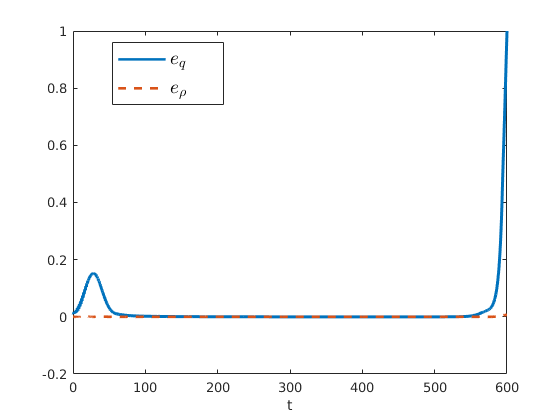
In order to verify this numerically, we discretized (88) using finite differences with a first order explicit in time and implicit in space upwind scheme with $N_{x}=40$ discretization points in space, $N_{t}=816$ discretization points in time and the trapezoidal rule for the integration in (84). The same spatial discretization was used for the corresponding stationary optimal control problem. The discretized problems were both implemented in GAMS [10] and solved using the interior point method IPOPT [32]. The parameters for a numerical example are listed in Table 1. The numerical results for this example are presented in Figure 1 and show that the dynamic optimal solution is very close to the stationary solution for about two thirds of the considered time horizon. This justifies using for example feedback stabilization techniques to an optimal stationary state as a simple control principle as an alternative to solving a very difficult dynamical optimal control problem for gas pipeline operation.

Table 1: Choice of parameters for the numerical results in Figure 1

Symbol	Explanation	Chosen Value	Unit
$\theta$	friction factor	0.05	${\mathrm{m}}^{-1}$
$g$	gravitational constant	9.81	$\mathrm{m}\text{\,}{\mathrm{s}}^{-2}$
$h^{\prime}$	pipe slope	0.025	—
$c$	speed of sound	340	$\mathrm{m}\text{\,}{\mathrm{s}}^{-1}$
$L$	length of pipe	10 000	$\mathrm{m}$
$T$	length of time horizon	600	$\mathrm{s}$
$\rho^{0}_{L}$	initial density at the exit	35	$\mathrm{kg}\text{\,}{\mathrm{m}}^{-3}$
$q^{0}_{L}$	initial flux at the exit	400	$\mathrm{kg}\text{\,}{\mathrm{m}}^{-2}\text{\,}{\mathrm{s}}^{-1}$
$\rho^{T}_{L}$	desired density at the exit	40	$\mathrm{kg}\text{\,}{\mathrm{m}}^{-3}$
$q^{T}_{L}$	desired flux at the exit	400	$\mathrm{kg}\text{\,}{\mathrm{m}}^{-2}\text{\,}{\mathrm{s}}^{-1}$
$\alpha,\beta,\lambda$	weighting factors in cost function	0.01,0.01,0.1111	—

Refer to caption — Figure 1: The computed optimal flow $q$ (left) and optimal dynamic density $\rho$ (middle) and the relative error $e_{\rho}$ and $e_{q}$ compared to the optimal stationary state for the boundary trace at the entry (right)

0.6 Conclusions

We have shown that controls that solve optimal boundary control problems with linear hyperbolic systems have a turnpike structure in the sense that the $L^{2}$ –norm of the difference between the static optimal control and the dynamic optimal control remains uniformly bounded for arbitrarily long control times $T$ . Since the static optimal control is constant with respect to time, this means that the dynamic optimal control must approach this constant with increasing control time $T$ almost everywhere on the time interval $[0,\,T]$ . We have also given sufficient conditions for the turnpike phenomenon for optimal boundary control problems with an additional integer constraint. In this case the static problem is an optimization problem with an integer constraint and the turnpike phenomenon occurs if both the switching cost and the time interval $[0,\,T]$ are sufficiently large. It is not clear, if also for smaller penalty parameters in the switching penalization a turnpike phenomenon arises. This is a question for future research. Our results give important insights about the relation between the solutions of the dynamic optimal boundary control problems and the corresponding static optimal control problem. The results imply that for sufficiently large control times, the static optimal controls yield reasonable approximations for the dynamic optimal boundary controls.

Acknowledgment. This work is supported by DFG in the Collaborative Research Centre CRC/Transregio 154, Mathematical Modelling, Simulation and Optimization Using the Example of Gas Networks, project A03 and C03.

Bibliography

[1] R. A. Adams, J. J. F. Fournier, Sobolev Spaces, Academic Press, 2003.
[2] M. K. Banda, M. Herty and A. Klar, Coupling conditions for gas networks governed by the isothermal Euler equations, Networks and Heterogenous Media 1, (2006), 295-314.
[3] G. Bastin, J.-M. Coron, Stability and boundary stabilization of 1-d hyperbolic systems. Birkhäuser, Basel, Switzerland, 2016.
[4] G. Bastin, J.-M. Coron, B. d’Andrea-Novel, On Lyapunov stability of linearised Saint-Venant equations for a sloping channel, Networks and Heterogeneous Media 4, 177–187, 2009.
[5] J. Brouwer, I. Gasser, M. Herty, Gas Pipeline Models Revisited: Model Hierarchies, Nonisothermal Models, and Simulations of Networks, Multiscale Model. Simul., 9, 601–623, 2011.
[6] J.-M. Coron, Control and Nonlinearity, AMS, Providence, Rhode Island, 2007.
[7] T. Damm, L. Grüne, M. Stieler, K. Worthmann, An exponential turnpike theorem for dissipative discrete time optimal control problems, SIAM J. Cont. Optim., 52, 1935–1957, 2014.
[8] R. Dorfman, P.A. Samuelson, R. M. Solow, Linear Programming and Economic Analysis, New York: McGraw-Hill, 1958.
[9] Faulwasser, T., Korda, M., Jones, C. N., Bonvin, D., On turnpike and dissipativity properties of continuous-time optimal control problems, Automatica, 81, 297-304, 2017.
[10] GAMS Development Corporation, General Algebraic Modeling System (GAMS), 2014, Release 24.3.3, Washington, DC, USA.
[11] L. Grüne, S. Pirkelmann, M. Stieler, Strict dissipativity implies turnpike behavior for time-varying discrete time optimal control problems Preprint, Bayreuth, 2017.
[12] M. Gugat, M. Herty, Existence of classical solutions and feedback stabilization for the flow in gas networks, ESAIM: COCV, 17 (2011) 28–51.
[13] M. Gugat, M. Herty, V. Sacher, Flow control in gas networks: exact controllability to a given demand. Mathematical Methods in the Applied Sciences 34, (2011), 745–757.
[14] M. Gugat, M. Dick and G. Leugering, Gas Flow in Fan-Shaped Networks: Classical Solutions and Feedback Stabilization, SIAM J. Control Optim., 49, 2101–2117, 2011.
[15] M. Gugat, E. Trélat, E. Zuazua, Optimal Neumann control for the 1D wave equation: Finite horizon, infinite horizon, boundary tracking terms and the turnpike property. Systems and Control Letters 90, 61-70, (2016). https://dx.doi.org/10.1016/j.sysconle.2016.02.001.
[16] M. Gugat, E. Zuazua, Exact penalization of terminal constraints for optimal control problems, Optimal Control Applications and Methods, 1099-1514, 2016.
[17] F. M. Hante, Relaxation Methods for Hyperbolic PDE Mixed-Integer Optimal Control Problems. Optimal Control Applications and Methods, Vol. 38(6), 1103–1110, 2017.
[18] F. M. Hante et al., Challenges in optimal control problems for gas and fluid flow in networks of pipes and canals: From modeling to industrial applications, in Industrial Math. and Complex Sys., P. Manchanda et al. (Eds.), Springer Singapore, 77–122, 2017.
[19] F. M. Hante, G. Leugering, T. I. Seidman, Modeling and Analysis of Modal Switching in Networked Transport Systems, Appl. Math. Opt. 59, 275–292, 2009.
[20] A. Hasan, L. Imsland, I. Ivanov, S. Kostova, B. Bogdanova, Optimal Boundary Control of 2x2 Linear Hyperbolic PDEs, 2016 24th Mediterranean Conf. Cont. Automat. (MED), DOI: 10.1109/MED.2016.7536012.
[21] R. L. Higdon, Initial-Boundary Value Problems for Linear Hyperbolic Systems, SIAM Rev. 28, 1986.
[22] L. Hörmander, Lectures on Nonlinear hyperbolic Differential Equations, Springer, Paris, 1997.
[23] I. Kazufumi, K. Kunisch, Multiplier approach to variational problems and applications Advances in Design and Control, Vol. 15, SIAM, Philadelphia, PA (2008)
[24] I. Lasiecka and R. Triggiani, Control Theory for Partial Differential Equations, Volume 2, Abstract Hyperbolic-like Systems over a Finite Time Horizon, Cambridge University Press, Cambridge, UK, 2000
[25] G. Leoni, A first Course in Sobolev Spaces, American Mathematical Society, Providence, Rhode Island, 2009.
[26] A. Porretta and E. Zuazua, Long Time versus Steady State Optimal Control, SIAM J. Control and Optimization 51, 4242–4273, 2013.
[27] A. Porretta and E. Zuazua, Remarks on Long Time Versus Steady State Optimal Control, in Mathematical Paradigms of Climate Science 15, Springer INdAM Series, 67–89, 2016.
[28] E. Trélat, E. Zuazua, The turnpike property in finite-dimensional nonlinear optimal control, J. Differential Equations 258, 81–114 (2015).
[29] E. Trélat, C. Zhang, E. Zuazua, Steady-state and periodic exponential turnpike property for optimal control problems in Hilbert spaces (arXiv:1610.01912)
[30] E. Trélat, C. Zhang, Integral and measure-turnpike properties for infinite-dimensional optimal control systems, Mathematics of Control, Signals, and Systems 30.3, 2018.
[31] E. Trélat, C. Zhang, E. Zuazua, Optimal shape design for 2D heat equations in large time, 2017, hal-01442997.
[32] A. Wächter, L. T. Biegler, On the Implementation of a Primal-Dual Interior Point Filter Line Search Algorithm for Large-Scale Nonlinear Programming, Math. Progr. 106, 25–57, 2006.
[33] A. Zaslavski, Existence and Structure of Optimal Solutions of Infinite-Dimensional Control Problems, Appl. Math. and Optim. 42, 291–313, 2000.
[34] F. Zhu and P. J. Antsaklis, Optimal control of hybrid switched systems: A brief survey, Discrete Event Dynamic Systems, 1–20, 2014.
[35] E. Zuazua, Large time control and turnpike properties for wave equations, Annual Reviews in Control 2017.

			$\displaystyle\int_{0}^{L}\frac{1}{2}\\|f(t,\,x)\\|^{2}_{\mathbb{R}^{2}}\,dx-\int_{0}^{L}\frac{1}{2}\\|f(t-1,\,x)\\|^{2}_{\mathbb{R}^{2}}\,dx$
		$\displaystyle\geq$	$\displaystyle\frac{1}{2}\,d_{+}(0)\,\int_{t-1}^{t}f_{+}(s,0)^{2}\,d\tau+\frac{1}{2}\,\|d_{-}(L)\|\,\int_{t-1}^{t}f_{-}(s,L)^{2}\,d\tau+\int_{t-1}^{t}\int_{0}^{L}f^{\top}\left(\|\eta_{0}\|\,\,M^{\top}-\frac{1}{2}D^{\prime}\right)f\,dx\,d\tau$
		$\displaystyle\geq$	$\displaystyle\frac{1}{2}\,d_{+}(0)\,\int_{t-1}^{t}f_{+}(s,0)^{2}\,d\tau+\frac{1}{2}\,\|d_{-}(L)\|\,\int_{t-1}^{t}f_{-}(s,L)^{2}\,d\tau-\frac{\tilde{C}_{2}}{2}\,\left\\|y_{0}^{(t)}\right\\|^{2}_{(L^{2}(0,\,L))^{2}}.$