June 2018
Classification
of Left-Right Symmetric Heterotic String Vacua
Alon E. Faraggi1**
*
E-mail address: alon.faraggi@liv.ac.uk
Glyn Harries1††
†
E-mail address: g.harries@liv.ac.uk and John
Rizos2‡‡
‡
E-mail address: irizos@uoi.gr
1 Dept. of Mathematical Sciences, University of Liverpool, Liverpool
L69 7ZL, UK
2 Department of Physics, University of Ioannina, GR45110 Ioannina,
Greece
The classification method of the free fermionic heterotic string vacua is extended to models where the GUT symmetry is broken directly at the string scale to the Left-Right Symmetric subgroup. Our method involves using a fixed set of basis vectors which are defined by the boundary conditions assigned to the free fermions before enumerating the string vacua by varying the Generalised GSO (GGSO) projection coefficients. It allows the derivation of algebraic expressions for the GGSO projections for each sector that generates massless states in the models. This enables a computerised analysis of the entire massless spectrum of a given choice of GGSO projection coefficients. The total number of vacua in the class of models chosen is . A statistical sampling is performed and a sample size of vacua with the Left-Right Symmetric gauge group is extracted. We present the results of the classification, noting that contrary to the previous classification of Pati-Salam models, no three generation exophobic models were found. The results obtained demonstrate the existence of three generation models with the necessary Higgs representations needed for viable spontaneous symmetry breaking, and with a leading top quark Yukawa coupling.
1 Introduction
The Standard Model of particle physics provides viable perturbative parameterisation of all subatomic observable data. The perturbative logarithmic evolution of the Standard Model parameters hints that the Standard Model may persist in providing viable parameterisation up to the Planck scale, where the gravitational interaction becomes of comparable strength. Further elucidation of the Standard Model parameters therefore necessitates the synthesis of the Standard Model with gravity. Contemporary string theories provide consistent perturbative frameworks to study this synthesis. They are chiral and free of gauge and gravitational anomalies. String theories are the only contemporary theories that achieve this feat, and therefore provide a superior framework to study the synthesis of the Standard Model with gravity. Furthermore, the Standard Model matter charges strongly hint at the realisation of Grand Unified Theory (GUT) multiplet structure in nature. By accommodating spinorial 16 representations in its perturbative spectrum, the heterotic string incorporates the –GUT picture [1]. A key prediction of the –GUT theory is that the Weinberg angle at the unification scale is given by , which is compatible with the low energy data.
The string consistency conditions introduce additional degrees of freedom beyond those of the Standard Model. These may be interpreted as a number of extra spacetime bosonic coordidates, or as a finite number of free, or interacting, fields propogating on the string worldsheet. String vacua are obtained by specifying these extra degrees of freedom, subject to the string consistency conditions. A priori the number of possibilities is vast and there is no clear guiding principle to select among them. The best we can accomplish at present is to extract features of classes of compactifications and to develop the methodolgy to discern between different classes [2]. The toroidal orbifolds represent one such class of models that has been studied in detail [3]. This class of compactifications gives rise to an abundance of viable three generation models with different unbroken subgroups of , and the canonical –GUT prediction . Among the distinct features of the class of orbifolds we note the spinor–vector duality [4, 5], that generalises to other classes of string vacua [6]; the existence of exophobic vacua [7]; and the possibility to fix all geometric moduli by asymmetric assignment of worldsheet boundary conditions [8]. The torodial orbifolds have been studied primarily by using the free fermionic formulation of the heterotic–string in four dimensions [9]. These models correspond to toroidal orbifold compactifications at special points in the moduli space with discrete Wilson lines [3]. Since the twisted matter spectrum in the orbifolds is independent of the moduli, analysing these models at the free fermionic point captures the phenomenological properties of the physical spectrum. Deformations away from the free fermionic point are obtained by adding worldsheet Thirring interactions [10]. The fermionic formulation facilitates the analysis of the spectrum and interactions, but the physical properties of this class of string vacua are rooted in the orbifold structure.
Three generation free fermionic models have been constructed since the late eighties. The early viable constructions provided isolated examples with (FSU5) [11], (PS) [12], (SLM) [13] and (LRS) [14], unbroken subgroups of . All with the canonical embedding of the weak hypercharge, yielding the GUT prediction for the Weinberg angle at . The case of the (SU421) subgroup was shown not to produce viable models [15, 16]. Over the past two decades systematic methods to classify large spaces of free fermionic models were developed, [17, 18, 4, 7, 19, 20, 21], culminating in the classification of Standard-like Models [22]. The initial application was for type II superstring vacua [17], and was extended to the classification of heterotic–string vacua with unbroken symmetry in refs. [18, 4]. This led to the discovery of spinor–vector duaility in the space orbifolds with worldsheet supersymmetry [4, 5]. The classification method provides an effective trawling algorithm to construct string models with specific phenomenological properties. Examples include: the construction of exophobic heterotic–string vacua [7]; the construction of heterotic–string vacua with GUT group [19]; the construction of string vacuum that allows a family universal extra vector boson with embedding to remain unbroken down to low scales [23].
In this paper we extend the classification methodology to the class of free fermionic heterotic–string vacua in which the gauge group is broken to the left–right symmetric extension of the Standard Model gauge group. From a phenomenological low energy point of view, this extension of the Standard Model is highly motivated [24] and dates back to the mid–70s, when the gauge and matter structure of the Standard Model crystallised. The left–right symmetry naturally explains the generation of parity violation in nature, via the spontaneous symmetry breaking of . It represents a rather minimal extension of the Standard Model, that avoids the tight constraints imposed from proton lifetime limits on the scale of other extensions. Thus, the spacetime vector bosons of the enhanced symmetry may exist below, say, 100TeV and appear in future experiments. From the point of view of the string model building this class of models introduces novel characteristics that were highlighted in ref. [14]. The basic contrast from the FSU5, PS and SLM models is that the LRS models of ref. [14] do not possess the embedding of the Standard Model states. This results in left-right symmetric models that do not have an anomalous symmetry, which appears in the others cases. In that respect the LRS models of ref. [14] possess a similar structure to the SU421 models of ref. [15, 16] that were shown not to admit viable three generation models. These properties of the LRS free fermionic models may be traced to the absence of an –map [25] in the LRS models of ref. [14]. By contrast the LRS models that we construct herein do possess an –map, which represents a vital step in the classification methodology. In that respect the models that we analyse in this paper are distinct from those of ref. [14].
Our paper is organised as follows: in section 2 a brief introduction to the construction of free fermionic models is given. The set of basis vectors used to generate models are presented, before outlining the construction of the LRS models in the ensuing discussion. Section 3 presents details of the string spectrum, such as the untwisted gauge symmetry of the LRS models and enumeration of the sectors that can enhance it. Section 4 provides a complete description of the twisted matter spectrum. This includes the observable, exotic and hidden matter sectors. Section 5 details the results of the classification and contains analysis of the data while providing comparisons to earlier classifications [7, 20, 22]. In section 5.3 we give the GGSO projection coefficients of a phenomenologically viable LRS heterotic–string model. In our examplery model all enhancing vector bosons are projected out. It contains three chiral generations, no chiral exotics as well as heavy and light Higgs multiplets, required for viable spontaneous symmetry breaking and fermion masses. Section 6 concludes the paper.
2 Left Right Symmetric Free Fermionic Models
This paper concerns the extension of the free fermionic classification method, utilised in [18, 4, 7, 20, 22], to vacua which possess the Left-Right Symmetric (LRS) subgroup of . The free fermionic models correspond to orbifold compactifications with superconformal worldsheet supersymmetry and discrete Wilson lines. The formulation of the free fermions occurs at an extented symmetry point in the moduli space where the compactified directions are interpreted as two dimensional fermionic degrees of freedom which propagate on the string worldsheet.
The free fermionic formulation provides a set of rules which enables extraction of the physical states in a string model and provides a straightforward approach to studying the phenomenological properties of the string vacua. The models are constructed by defining a set of basis vectors and the Generalised Gliozzi-Scherk-Olive (GGSO) projection coefficients of the one-loop partition function. The details are outlined in the following section.
The breaking of the GUT symmetry occurs directly at the string scale. All the models which are classified possess spacetime supersymmetry and preserve the embedding of the weak hypercharge. The unbroken subgroup of in the low energy effective field theory considered here is . The matter states which give rise to the Standard Model fermionic representations are found in the spinorial 16 representation of decomposed under the unbroken subgroup. Similarly, the SM light Higgs states occur from the vectorial 10 representation of .
2.1 The Free Fermionic Formulation
The notable features of the free fermionic formulation used in model building and classification will be briefly outlined. A more detailed discussion of these features can be found in reference [9].
The free fermionic formulation of string theory is directly formulated in four space-time dimensions, whereby the extra degrees of freedom found in string theories are interpreted as free fermions propagating on the two dimensional string worldsheet. The approach considered here utilises the four dimensional heterotic string in the light cone gauge, meaning there are 20 left moving and 44 right moving free fermions introduced to account for all the extra degrees of freedom. In the standard notation the left movers are represented by and the right movers by .
When these fermions are parallel transported around the two noncontractible loops of the one-loop partition function, they obtain a non-trivial phase11 1 In the common nomenclature, these phases are also referred to as ‘boundary conditions’ of the free fermions.. These phases can be either periodic, anti-periodic or complex, denoted by 0,1 and respectively. The boundary conditions of the fermions are specified in 64-dimensional vectors called ‘basis vectors’ which are given in the form
where the boundary condition is defined as the transformation property for a fermion . Accordingly,
Each model is specified by a set of basis vectors , which must satisfy modular invariance constraints. The basis vectors of the model span a space , which consists of sectors. Each sector is formed as a linear combination of the basis vectors and is given by
| (1) |
where . The string states in each sector, denoted by , must also conform to modular invariance constraints. This is imposed on the string states in the form of the one-loop GGSO projections via the equation,
| (2) |
where is the fermion number operator, is the space-time spin statistics index and is the GGSO projection coefficient. By varying the choice of the GGSO coefficients, distinct vacua of the string model are obtained.
Summarising, a model is constructed by using a set of basis vectors and a set of distinct GGSO projection coefficients , with , of which there are .
2.2 Models
In order to build the Left-Right Symmetric models that are studied in this paper, a set of thirteen basis vectors are used. The first twelve basis vectors considered generate models and are common in the previous publications [7, 20, 22, 16]. These basis vectors are also included in the basis of the LRS models discussed here and are defined as:
| (3) | |||||
where and the fermions which appear in the basis vectors have periodic (Ramond) boundary conditions, whereas those not included have antiperiodic (Neveu-Schwarz) boundary conditions.
The basis vector is required by the rules set out in the papers listed in reference [9] and generates a model with an gauge group from the Neveu-Schwarz (NS) sector. Addition of the basis vector generates space-time supersymmetry and leaves the gauge group intact. The vectors break the gauge group to but preserve the supersymmetry. These vectors correspond to all the possible internal symmetric shifts of the six internal bosonic coordinates. Addition of the vectors and corresponds to orbifold twists and breaks the space-time supersymmetry firstly to and subsequently to . They also break the gauge symmetry, therefore reducing the rank of the gauge group, while simultaneously decomposing the to . Addition of the basis vectors and then break the hidden gauge group, generated by the fermions , to . The untwisted vector bosons present due to this choice of basis vectors generate the gauge group in the adjoint representation.
2.3 Left-Right Symmetric Models
Previous constructions of free fermionic LRS models used two or more basis vectors to break the observable gauge group. Firstly, one basis vector with either the assignment (as in [14]), or equivalently (as in [7]), is used to obtain the Pati-Salam gauge group and a second basis vector with the assignment breaks the Pati-Salam gauge group to the LRS.
However, the model under consideration here uses only one additional basis vector, given by
| (4) |
where the restriction that the phase on the complex right-moving fermions is positive is made, i.e . The assignment of is made due to the contraint that , where , must be true in order to satisfy modular invariance.
It should be noted that while the assignments on the fermions must be as above, this choice of is not unique due to possible variations of assignments for the fermions . However, in this paper only models with the defined above are considered.
With this choice of basis vectors, we note two sectors which are combinations of the basis vectors and facilitate the classification and presentation of the physical spectrum. The first is the composite vector defined as ‘’ which is given by
| (5) |
This combination of basis vectors corresponds to the third twisted plane of the orbifold, where the first two are related to and , respectively. The second is given by the linear combination denoted by ‘’, given by
| (6) |
This linear combination produces the spinorial 128 multiplet in the 248 adjoint representation of the observable , generated by the subset of the basis set (3). It generates the so–called –map [25] that exchanges spinorial and vectorial representations from the twisted sectors , to be defined below, and , respectively. We remark that this linear combination is not generated in the LRS models of ref. [14] and therefore the models presented there do not admit the –map. This is an important distinction between the models considered here and those of ref. [14]. We note that the –map is crucial in our classification method as the sectors are those that give rise to the Standard Model electroweak doublets. Therefore, the basis of the models considered consists of the basis vectors with two notable linear combinations .
2.4 GGSO Projections
Now that the basis has been specified, the next components of the model which need defining are the GGSO projection coefficients which are necessary in order to completely describe the one-loop partition function.
The GGSO coefficients span a matrix. The lower triangle of the matrix containing 78 coefficients is fixed by the corresponding 78 coefficients in the upper triangle by modular invaraince constraints. In addition, the phases on the diagonal are also fixed by modular invariance. Accordingly,
| (7) |
To ensure supersymmetry, without loss of generality, the following coefficients are fixed
| (8) |
where and . We are therefore left with 66 independent coefficients, which generates distinct string vacua.
It should be noted that all the phases are real and take the discrete values except for the phase which takes values due to the fact that .
3 String Spectrum
Adapting the methodology of previous cases [7, 16, 20, 22], the sectors which can contribute massless states are enumerated and the corresponding algebraic conditions for the GGSO projections are derived for each sector.
Spacetime vector bosons that arise from the the untwisted sector, generate the symmetry and its unbroken subgroups. There are further sectors in these models that can give rise to additional physical spacetime vector bosons, which enhance the untwisted gauge symmetry. Furthermore, if the additional spacetime vector bosons are charged with respect to the Cartan generators of the GUT symmetry, the unbroken subgroup is enhanced. Thus, a pivotal requirement in the construction is that the additional spacetime vector bosons are projected out.
The twisted sectors produce matter multiplets which possess supersymmetry and can be grouped depending on which subgroup they leave unbroken. Sectors which contain the basis vector in the linear combination break the symmetry to the LRS and gives rise to exotic states. If the linear combination contains then the gauge group is broken to the Pati-Salam gauge group and also contains exotics. As is the only breaking basis vector, all the remaining sectors which, a priori, do not include in the linear combination do not break the symmetry.
The sectors in a model can be catergorised according to the left and right moving vacuum. The physical states satisfy the Virasoro condition, defined as
| (9) |
where and are the sums over the left and right moving oscillators respectively. Sectors that have the products and can produce spacetime vector bosons, which determine the gauge symmetry in a given vacuum. Sectors where the products are and produce matter states which are outlined in section 4. All the models considered preserve spacetime supersymmetry, which is generated by the basis vector where the products are .
3.1 The Gauge Symmetry
Vector bosons from the untwisted sector correspond to generators of the following observable and hidden gauge group symmetries
| Observable | (10) | ||||
| Hidden | (11) |
and the weak hypercharge is given by22 2 It should be noted that and
| (12) |
Depending on the choice of GGSO projection coefficients, additional space-time vector bosons may arise from the following 26 sectors
| (13) |
where is defined in equation (6). The sectors in (13) have been organised such that the sectors which do not break the symmetry are on row 1; rows 2-3 break the symmetry to the Pati-Salam gauge group and finally rows 4-7 break the symmetry to the LRS gauge group.
We remark that any projections on sectors containing can be inferred from the projections made on the corresponding sector which contains only . Therefore, in the following analysis these sectors will not be discussed in detail.
If any of the gauge bosons from the sectors in eq. (13) survive the projections, the untwisted gauge symmetry is enhanced. We restrict the classification analysis to vacua with no enhancements, meaning that the gauge symmetry of all the vacua classified is identical. In the classification method the GGSO projection coefficients of the 26 sectors listed above were derived and expressed in an analytic form so that a computer code can easily detect if a particular vacua is enhanced. Of the vacua that were scanned in the classification, approximately contained extra vector bosons and were therefore enhanced.
4 The Twisted Matter Spectrum
4.1 General Remarks
In the table below, the hypercharge and electromagnetic charge have been normalised according to the equations
| (14a) | |||
| (14b) |
In these equations, the charges are the charges generated by the fermions respectively and are calculated according to the equation
| (15) |
where is the boundary condition of the fermion in the sector and is the fermion number given by
| (16a) | |||
| for fermionic oscillators and their complex conjugates, and | |||
| (16b) | |||
for the degenerate Ramond vacua where is a degenerated vacuum with no oscillator and is the degenerated vacua with one zero mode oscillator.
The table below outlines the electromagnetic charges, and the charges under the electroweak Cartan generators, of the states which are contained in the observable LRS chiral matter representations:
| Representation | ||||
|---|---|---|---|---|
| () | 1/6 | 2/3 , -1/3 | ||
| () | 2/3 | 2/3 | ||
| () | -1/3 | -1/3 | ||
| () | -1/6 | 1/3 , -2/3 | ||
| 1/3 | 1/3 | |||
| -2/3 | -2/3 | |||
| 1/2 | 1 , 0 | |||
| 1 | 1 | |||
| 0 | 0 | |||
| -1/2 | 0 , -1 | |||
| 0 | 0 | |||
| -1 | -1 |
where the representation is decomposed as . The notation ‘’ above denotes a state of the degenerated Ramond vacua with no oscillator, i.e a state with a fermion number , whereas the notation ‘’ denotes a state of the degenerated Ramond vacua with a zero mode oscillator and therefore a state where . The values for and are calculated using equations (14a) and (14b) respectively.
It is when these representations are decomposed under the SM gauge group that we get the particle states of the Standard Model. The leptons and quarks are realised by the following representations
| (17a) | |||
| (17b) | |||
| (17c) | |||
| (17d) | |||
| (17e) |
where and are the low energy supersymmetric superfields associated with the Minimally Supersymmetric Standard Model (MSSM).
4.2 The Observable Matter Sectors
The chiral matter spectrum is obtained from the twisted sectors, which are as follows
| (18) | |||||
where and . These 48 sectors contain the 16 and spinorial representations of the observable gauge group decomposed under as
We remark that in this construction, each of the sectors with , can contribute at most a single multiplet to the physical spectrum. The integers essentially label the sixteen fixed points of the twisted plane. For this reason we can interchange the identification of the –sectors with states in the physical spectrum, i.e. the spectrum of states that survive the GGSO projections. The power of the formalism is that all the states producing sectors can be expressed in a similar fashion.
In addition to the twisted matter spectrum, there are vector-like states which contribute to the observable matter spectrum. These states arise from the sectors
| (19) | |||||
which have four periodic right-moving complex fermions. Massless states can be obtained by acting on the vacuum with a Neveu-Schwarz right-moving fermionic oscillator. If the oscillator is from either the fermions or their complex conjugates then these sectors give rise to the vectorial 10 representation of decomposed under as
where the first and second representations are generated by the fermions and respectively and the final representation is generated by the fermions and . It can be seen that the first two representations are colour triplets, usually referred to as leptoquarks in the literature, which mediate proton decay via dimension five operators. Therefore, these states must be either sufficiently heavy so as to agree with the current proton lifetime of years [26] or must be projected out of the string spectrum by the GGSO projections. This is a constraint which is considered when the classification is performed. The representation give rise to the light Standard Model Higgs.
The remaining right-moving complex fermions can give rise to states which are singlets under the observable gauge group but form the following representations
- •
or , where is the degenerated Ramond vacuum of the sectors respectively. These states transform as vector-like representations of the ’s.
- •
or . These states transform as vector-like representations of the gauge group.
- •
or . These states transform as vector-like representations of the gauge group.
- •
or . These states transform as vector-like representations of the and gauge groups respectively.
4.2.1 Chirality Operators
In order to calculate the number of families of a model, the number of chiral 16 and representations of decomposed under the LRS gauge group have to be counted. In these models families and anti-families are formed from the following representations
| (20) |
A model must then have three families in order to be phenomenologically viable i.e
| (21) |
The number of these representations that occur in a model depends on the choice of the GGSO coefficients. Firstly, in order to distinguish between the 16 and an chirality operator is defined. These chirality operators for the sectors are defined, respectively, as
| (22) |
and can take the values . Another chirality operator needs defining to determine whether the representations or of the occur. These are defined for the sectors respectively as
| (23) |
where is the linear combination .
Furthermore, there is one final chirality operator which needs to be defined in order to determine the repesentations under the gauge group. These are
| (24) |
By performing the GSO projections of these chirality operators the surviving states and therefore the number of families are calculated.
4.2.2 Projectors
The projectors are a set of equations which determine whether a sector is either projected out or kept in the string spectrum. These projectors consist of the relevant GGSO coefficients for the sector. For the observable chiral matter there are 48 projectors which are calculated to be
| (25) |
The analysis of the physical spectrum is formulated as algebraic equations. The projectors can be expressed as a system of linear equations where take unknown values. The sectors which survive the GSO projections are found by solving the systems of equations for . Using this formalism allows for a computer analysis of the models as the systems of linear equations are easy to express in a computer code.
The following notation is used in the algebraic representation of the GGSO projections
| (26) |
When the GGSO coefficients are expressed in this way the analytic expressions for the projectors are given in matrix form as
respectively. Such algebraic matrix equations can be written for the entire physical spectrum. In the ensuing discussion we list all the sectors that can a priori produce physical states, but do not list explicitly all the algebraic matrix equations for the corresponding GGSO projections.
4.3 Exotic Sectors
Additional sectors exist in the string models that can give rise to states that carry fractional charges under the LRS gauge group. This leads to states with a fractional electric charge at the level of the Standard Model. The term ‘exotic states’ used here is reserved purely for the states with fractional electric charge which arise from the sectors containing the basis vector . Exotic states arise from these sectors due to Wilson line breaking of the non-Abelian GUT symmetries. These exotics states are a generic feature of string compactifications [27, 28, 29] and experimental searches are being conducted in order to find them [30]. There are interesting phenomenological aspects to exotic states as charge conservation implies that the lightest of these states is necessarily stable. To date however, no such exotic states have been observed, leading to strong upper bounds on their abundance [30]. In addition, if these states are too plentiful in the early universe they can cause problems during the reheating phase as the lightest of these states is necessarily stable, meaning they continue to scatter and cannot decouple from the plasma in the early Universe due to their charge.
There are two solutions to the lack of experimental data for the existence of exotics. The first solution is by demanding that the exotics are confined to integrally charged states [11]. The second is to demand that the exotic states are sufficiently heavy and diluted in the cosmological evolution of the universe [29]. However, there are issues with the integrally charged state solution as these states affect the renormalisation group running of the weak-hypercharge and gauge group unification. This leads to the preferred solution of demanding that the exotic states are sufficiently massive and dilute. A sufficient mass for these states is above the GUT scale so that they are diluted during the inflationary period of the universe as during the reheating phase they will not be reproduced.
Previous classifications of heterotic-string models found examples of vacua in which massless exotics states were absent and only appeared in the massive spectrum. These models were dubbed ‘exophobic heterotic string vacua’. In the case of the Pati-Salam models, three generation exophobic vacua were found [7] and in the FSU5 case exophobic vacua were found in models with an even number of generations [20]. A question of interest for the current research is therefore whether any exophobic LRS models can be found.
4.3.1 Spinorial Exotics
The term spinorial exotics refers to sectors which involve the basis vector and have the products and , therefore requiring no oscillators to produce massless states.
The sectors below all give rise to states with the representations and under the observable gauge group. These states are defined in the analysis as and respectively. It can be seen that these are singlets under the gauge group but are still charged under . The corresponding sectors with in the linear combination of basis vectors give states with the representations and . It can be seen that the only change is the sign reversal of the charge under . The following are the sectors which give rise to these representations
| (27) | |||||
| (28) | |||||
| (29) | |||||
| (30) | |||||
4.3.2 Vectorial Exotics
The following are vectorial states, meaning they have the products and , therefore requiring one oscillator to produce massless states. Firstly, there are the sectors
| (31) | |||||
Using as an example to show the states that can be obtained from these sectors, the possible states are
- •
, where is the degenerate Ramond vacua of the sector. These states transform as vector-like representations of the observable .
- •
. These states transform as vector-like representations of .
- •
. These states transform as vector-like representations of and respectively.
- •
. These states transform as vector-like representations of the hidden .
- •
. These states transform as vector-like representations of the hidden .
The states obtained from the sectors transform in the same manner as those above.
Secondly, there are the following 48 sectors
| (32) | |||||
The states found from these sectors only differ from by a negative sign on the boundary conditions of the fermions . This has the effect of changing the sign of the charges while leaving the other charges unaffected. The structure and charges generated by the other worldsheet fermions therefore remain identical.
Similarly, in the sectors
| (33) | |||||
the observable states are identical to those in the sectors and only the hidden charges differ by a slight change in the Ramond vacua and a sign difference of the boundary conditions of the fermions , which only affects the sign of the charges under .
The final 48 sectors are
| (34) | |||||
These differ from sectors by changing the sign on the boundary conditions of the fermions and therefore, as above, there is a sign change on the charges under . All other states are unaffected and remain as in the sectors .
4.3.3 Pati-Salam Exotics
In the case of left-right symmetric models, there can be states which are exotic with respect to the Pati-Salam gauge group . The sectors from which these states can arise are those which contain the vector combination . This is due to the fermions or having periodic boundary conditions in the sector (therefore generating the Pati-Salam gauge subgroup), while still having a fractional electric charge with respect to the Standard Model.
In the model being discussed, all of the Pati-Salam exotics are found in the following sectors:
| (35) | |||||
These states transform in representations of the gauge group .
| (36) | |||||
These states transform as representations of the gauge group . The states from the previous 96 sectors are defined in the analysis as and .
| (37) | |||||
These states transform as representations of the gauge group
| (38) | |||||
These states transform as representations of the gauge group . The states from the previous 96 sectors are defined in the analysis as and .
4.4 Hidden Matter Spectrum
The hidden matter spectrum refers to sectors which produce states that transform under the hidden gauge group but are singlets under the observable SO(10) GUT gauge group. This means that the states produced are not exotic with respect to the Standard Model gauge charges.
There are 48 sectors present from which are
| (39) | |||||
These sectors contain states which transform under the hidden gauge group with the representations , , , , .
There exists another 48 sectors given by
| (40) | |||||
These sectors produce states which transform under the gauge group with the representations: , , where the charges of and can take all possible permutations of the values given, meaning there are 12 distinct representations in total.
5 Classification Results and Analysis
The classification process involves utilising the calculated algebraic conditions which were presented in the previous sections. By using the projectors and chirality operators for each sector the entire massless spectrum can be analysed for a specific choice of the one-loop GGSO projection coefficients. These algebraic conditions can be written in a computer program which enables a scan over the different choices of GGSO projection coefficients. As the total number of possible configurations, and therefore vacua, is a complete scan of the entire space of string vacua is not possible. Therefore, a random generation of the GGSO projection coefficients is used in order to provide a random sample of vacua33 3 We note here that analysis of large sets of string vacua have been performed by other research groups [31] from which models with desirable phenomenological criteria can be found.
The algebraic conditions were programmed into a JAVA code in order to perform the classification and the accuracy of this program was checked against an independently written FORTRAN code. In the JAVA program, a random generator was used in order to provide the different GGSO configurations. This program initially produces a random GGSO configuration, before running these values through the algebraic conditions calculated for each sector in order to produce the full spectrum of each model. By repeating this process, the statistics associated with classification can be developed while also fishing for single models which are of phenomenological significance.
Previous papers which have utilised this technique can be seen in references [7, 16, 20, 22]. In the case of the classification of Pati-Salam models, this method was shown to produce three-generation models which contained no exotic massless states with fractional electric charge, and were therefore exophobic.
Therefore, an example of a question of phenomenological interest is whether exophobic LRS models can be found.
| Spinorial | Vectorial | LRS Exotic | Pati-Salam Exotic |
| Observable | Observable | ||
The observable sector of a heterotic-string Left-Right Symmetric model is characterised by 27 integers which are defined in table 1. These contain the relevent quantities of phenomenological interest. Notable numbers defined in table 1 are , and as these give the number of generations of a model and whether the model contains non-chiral light and heavy Higgs representations.
The numbers given in the first two columns of table 1 are as described above in section (4.2). The first four numbers form a complete 16 of and the last four form a complete . The first four in the LRS Exotics column arise from the spinorial exotic sectors and the last two arise from the vectorial exotic sectors. To perform the classification, the analytic formulae for all the sectors which contribute to these numbers were derived so as to describe the complete spectrum of each model.
For a model to be phenomenologically viable, it must satisfy the following phenomenological criteria:
| Three light chiral generations | ||||
| At least one heavy Higgs pair to break the symmetry | ||||
| At least one light Higgs bi-doublet | ||||
| Heavy mass can be generated for the colour triplets | ||||
| Heavy mass can be generated for the colour triplets | ||||
| Heavy mass can be generated for vector-like exotics | ||||
| Heavy mass can be generated for the colour triplets | ||||
| Heavy mass can be generated for the vector-like exotics | ||||
| Heavy mass can be generated for vector-like exotics | ||||
| Heavy mass can be generated for vector-like exotics |
where the contraints which generate the heavy masses have been imposed in order to generate LRS models which contain no chiral exotics.
An initial classification run of distinct models was performed and the results are displayed in section 5.2. Due to a relative lack in abundance of three generation models a second run of distinct models was performed with the constraints on the vector-like chiral exotic states relaxed. Namely, the condition that which arise from the Pati-Salam exotic sectors were relaxed, along with the conditions , and which arise from the LRS exotic sectors. We remark that whereas a run typically takes 2 days, a corresponding run can take 28 weeks, which becomes prohibitive. The results of these two runs is presented and commented on in section 5.2.
5.1 Top Quark Mass Coupling
For a model to be phenomenologically viable, it must reproduce the spectrum of the Standard Model while also reproducing the Standard Model interactions at the low energy limit. Therefore, our analysis extends to classifying the number of models which give the necessary conditions to include the top quark mass. In this class of models the top quark mass coupling is
where the superscripts and refer to the fermionic and bosonic components of the associated superfield respectively. It has been shown that the necessary conditions in order to have a top quark mass coupling can be imposed by a straightforward general analytical method [32]. This general method details, without loss of generality, that if , and arise from the sectors , and respectively, there exists a top quark mass coupling.
5.2 Results
We now explore the space of the Left-Right Symmetric free fermionic heterotic string vacua. The sample size used in the first classification was vacua out of a possible total of . Some of the results are presented in Figures 1 - 3 and table 2.
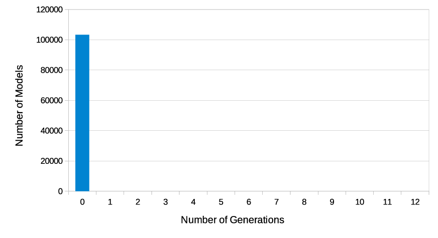
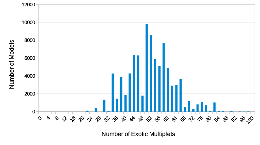
In Figure 1 the number of generations is presented against the natural logarithm of the number of models found. The results show the greatest number of models have zero generations and the number of models decreases as the number of generations increases. The maximum number of generations found was . Figure 2 shows that only exophobic models with zero generations were found. Figure 3 displays the number of three generation models with no chiral exotic multiplets found with respect to the total number of exotic multiplets they contain. The results show minimally exotic models to have 22 exotic multiplets while maximally exotic models have 90 exotic multiplets. The greatest number of models contained 50 exotic multiplets and the results show an approximately normal distribuition, skewed slightly to models containing more than 50 multiplets. It can be seen in table 2 that of the non-enhanced models with complete families had no chiral exotics. The inclusion of the constraint demanding that the model must have three generations then drastically drops the probability of finding a viable model. The probability of finding a model which satisfies all these criteria is . Of these models, the probabilities that they contain no Higgs particles, only SM light Higgs particles or only heavy Higgs particles are , and respectively. Table 2 shows that requiring the model to contain both a light SM Higgs and a heavy Higgs yielded one model. Although this suggests models with interesting phenomenology exist, this result is not statistically significant and therefore does not allow meaningful conclusions to be drawn. This result also does not allow for any analysis involving further constraints.
Due to the lack of models with suitable phenomenology found during the sample, the sample size was increased to and some of the constraints were relaxed. Specifically, the constraints concerning the chiral exotic triplets in the models were included (i.e and ), whereas the contraints concerning the vector-like chiral color–singlet exotics were omitted. We note that relaxing these constraints entails that in some of the scanned models is anomalous.
| Constraints | Total models in sample | Probability | Estimated number of models in class | |
| No Constraints | ||||
| (1) | + No Enhancements | |||
| (2) | + Complete Families | |||
| (3) | + No Chiral Exotics | |||
| (4) | + Three Generations | |||
| (5) | + SM Light Higgs | |||
| + & Heavy Higgs | ||||
| (6) | + Minimal Heavy Higgs | 0 | ||
| & Minimal SM Light Higgs | ||||
| (7) | + Top Quark Mass Coupling | 0 |
The sample size was then increased to perform a classification on vacua out of a possible total of and the program was run again. Some of the results are presented in Figures 4 - 6 and Tables 3 - 4.
In Figure 4 the number of models versus the number of full generations is displayed for the model run. The greatest number of models can be seen to have zero generations and the number of models decreases as the number of generations increases. This result is in accordance with the run and the previous results of classifications [7, 20, 22]. It can be seen that once the number of generations is greater than six, there is an absence of models. This result indicates that for this choice of basis vectors, models with are either completely forbidden or are extremely unlikely in the total space of model possibilities.
Figure 5 displays the number of exophobic models versus the number of generations. Analogously to the classification run, the results show a relative abundance of zero generation exophobic models but an absence of any exophobic models with . This result leads to the conclusion that there are no three generation exophobic models with a statistical frequency larger than . It should however be noted that the lack of exophobic models with does not suggest that exophobic Left-Right Symmetric models are completely forbidden, only that for the choice of basis vectors used in this analysis none were found with a reasonable statistical likelihood.
This result is in contrast to the case of the results of both the Pati-Salam and Flipped classifications [7, 20]. In the Pati-Salam case, exophobic models with were found and where exophobic models with an even number of generations were found with a notable absence for . In the flipped case, exophobic models with an even number of generations were found. While this means no three generation exophobic models were found, the flipped case admits many more exophobic models than the current LRS case.
In Figure 6 the total number of three generation models with matched number of colour triplets is displayed against the number of exotic fractionally charged multiplets in a given three generation model. It can be seen that the minimal number of exotic multiplets was again found to be 22, while the maximally exotic models contained 98, an increase from the previous run. The results again show a roughly normal distribution with a central peak at 50 exotic multiplets with a slight skew toward models where the number of exotic multiplets greater than 50. This result is similar to what was found in the classification of Pati-Salam models [7], but in the case of the LRS the average number of exotic multiplets is much higher. In the Pati-Salam case, there was a central peak at 18 exotic multiplets with maximally exotic models having 54 multiplets. This result is, in general, to be expected as in the LRS models both Pati-Salam and LRS exotic sectors exist, therefore there is the potential for many more exotic states to enter the spectrum.
Table 3 shows the number of non-enhanced three generation models which have matched numbers of colour triplets with respect to the number of Pati-Salam, spinorial and vectorial exotic multiplets. It can be seen that of the total number of models, there were models found which contained no spinorial exotic multiplets. This is also true in the case of vectorial exotic multiplets. However, no models were found which were exophobic with respect to the Pati-Salam exotic multipets, which is a leading reason for the lack of exophobic three generation models. This result is in contrast to the results of the classification performed in [7] as three generation exophobic Pati-Salam models were found.
Of the total models sampled, of the non-enhanced full generation models were found to have matched numbers of colour triplets. This is a slight increase from the classification run due to the relaxing of some of the conditions as mentioned previously. This can be seen in table 4. It should be noted that the probability of finding non-enhanced three generation models is actually lower in the classification run than in the case. This is expected to be a statistical fluctuation due to the random nature of the classification method. Further analysis on the effect of relaxing the requirement that all color–singlet exotics are vector–like in three generation models may be an interesting area of research. However, this is beyond the scope of this analysis and is left for future work.
If the constraint of having a top quark mass coupling is included, then of the total number of non-enhanced full generation models only were found to be viable. While three generation models with a top quark mass coupling were found, it can be seen from table 4 that their appearance was not found to be frequent, as the probability for finding such a model was found to be .
Of all the non-enhanced models with complete generations, contained at least one light Higgs. This is much higher than for the case of the heavy Higgs, where only of the total non–enhanced, generation complete models contained at least one heavy Higgs. When considering non–enhanced three generation models in which all exotic colour triplet are vector–like, the number which had at least one Standard Model Higgs is approximately and the number which had at least one heavy Higgs is approximately . Only of the non–enhanced three generation models with vector–like exotics contain both light and heavy Higgs multiplets. Comparing with previous classifications, we note that in the three generation Pati-Salam models classified in [7], had a heavy Higgs and of these had a SM Higgs. Whereas, in the flipped case [20], the non–enhanced and anomaly free three generation models had which contained a SM Higgs and contained a heavy Higgs. In comparison, it can be seen that the number of three generation free fermionic LRS models, free of anomalies and enhancements, which contain either Higgs is drastically lower. This outcome should nevertheless be compared with the case of the SU421 models in which no viable models can be constructed at all!
5.3 A Model of Notable Phenomenology
The random classification method can be used to trawl models with specified phenomenological properties. Using the notation convention
| (41) |
the model defined by the GGSO projection coefficients in eq. (42) provides an example of a non–enhanced three generation model, with potentially viable phenomenology.
| (42) |
The observable matter sectors of this model produce three chiral generations, a minimal SM Higgs () and a minimal heavy Higgs (). There exists colour triplets from the vectorial 10 representation of as and , but as there are equal numbers of them heavy mass can be generated and there exists no anomaly in the LRS gauge group from these sectors. This model also contains no enhancements. The numbers defined in table 1 for the spinorial LRS exotic sectors of this model are as follows: , . The vectorial LRS exotics have the values and . The Pati-Salam exotic states have the values , and . The model therefore has no anomaly under the LRS gauge group, i.e. all the exotic states are in vector–like representations, but does contain an anomaly under the and gauge groups. The model contains exotic multiplets and is therefore not exophobic. The model also admits a top quark mass coupling of order one.


| # Exotic Multiplets | Pati-Salam | Spinorial | Vectorial |
|---|---|---|---|
| 0 | 0 | 5536 | 1720 |
| 2 | 0 | 0 | 0 |
| 4 | 0 | 20854 | 3215 |
| 6 | 0 | 0 | 0 |
| 8 | 0 | 26727 | 19764 |
| 10 | 0 | 0 | 0 |
| 12 | 319 | 19102 | 4272 |
| 14 | 3030 | 0 | 0 |
| 16 | 894 | 10616 | 19750 |
| 18 | 15580 | 0 | 0 |
| 20 | 18598 | 1648 | 2157 |
| 22 | 13014 | 0 | 0 |
| 24 | 8703 | 3796 | 18673 |
| 26 | 15918 | 0 | 0 |
| 28 | 3528 | 739 | 1532 |
| 30 | 3386 | 0 | 0 |
| 32 | 1797 | 169 | 8093 |
| 34 | 2632 | 0 | 0 |
| 36 | 1169 | 0 | 952 |
| 38 | 398 | 0 | 0 |
| 40 | 25 | 73 | 7209 |
| 42 | 233 | 0 | 0 |
| 44 | 0 | 0 | 600 |
| 46 | 35 | 0 | 0 |
| 48 | 0 | 0 | 1212 |
| 50 | 1 | 0 | 0 |
| 52 | 0 | 0 | 9 |
| 54 | 0 | 0 | 0 |
| 56 | 0 | 0 | 46 |
| 58 | 0 | 0 | 0 |
| 60 | 0 | 0 | 40 |
| 62 | 0 | 0 | 0 |
| 64 | 0 | 0 | 16 |
6 Conclusion
The Standard Model of particle physics provides viable parameterisation of all subatomic observable data. Furthermore, the Standard Model may prevail in providing such effective viable parameterisation up to the GUT or Planck scales, where this necessarily breaks down due to quantum gravity effects. If this is the avenue chosen by nature, it is evident that further fundamental insight into the Standard Model parameters can only be gained by embedding it in a theory of quantum gravity. The synthesis of gravity and quantum mechanics is not yet an accomplished feat. There are various approaches and from a purely theoretical perspective all should be regarded on equal footing. String theory is among these approaches. String theory, however, has one key advantage. Its consistency conditions mandate the existence of the gauge and matter structures that appear in the Standard Model. Furthermore, these consistency conditions restrict the type and enumeration of states that can appear in the construction. String theory therefore provides the arena for the development of a phenomenological approach to the synthesis of gravity and the gauge interactions. Since the mid-eighties detailed quasi–realistic string models were constructed. A particular class of phenomenological string vacua are the orbifold compactifications that were constructed in the free fermionic formulation of the heterotic string.
In this paper we extended the classification of phenomenological free fermionic heterotic string vacua to models in which the –GUT group is broken to the Left–Right Symmetric (LRS), , subgroup. NAHE–based [33] LRS free fermionic models that utilise asymmetric boundary conditions were constructed in ref. [14]. The free fermionic classification method adopted herein utilise solely symmetric boundary conditions. The class of LRS vacua gives rise to several distinct features as compared to the FSU5, PS and SLM classes. In all the cases we may denote a basis vector that breaks the symmetry by . The difference between the FSU5, PS and SLM models versus the LRS and the SU421 models is that in the first case the vector does not break the symmetry, whereas in the second case it does. This distinction impacts the phenomenolgical characteristics of the two classes. In the case of the SU421 models the consequence is that it is not possible at all to construct SU421 free fermionic models with complete matter generations [15, 16]. Thus, a class of models that has attractive phenomenological features from a purely GUT–QFT perspective [34], cannot be constructed as an heterotic–string model, at least in the free fermionic formulation. By contrast, viable LRS free fermionic models can be constructed and in some abundance, as demonstrated in this paper. The key difference between the LRS and SU421 models is that in the later case the projection chooses either the left– or right–handed Standard Model representations, whereas in the former it does not. In the case of the LRS models there is a remaining freedom in the charges of the symmetries, , that produces opposite charges of the left– and right–handed Standard Model representations. This is in marked contrast with the corresponding charges in the PS, FSU5 and SLM models, in which they are necessarily the same. It would be of interest to explore how, and whether, these different cases are replicated in terms of bundles on complex manifolds.
The class of LRS free fermionic models that we explored herein differs from those of ref. [14]. The difference being that while the construction in ref. [14] does not admit an –map [25], the free fermionic classification methodology utilises this map. In this classification method the –map is used to generate the sectors that produce the Standard Model electroweak Higgs multiplets. The fact these LRS models do contain the –map, as well as the fact that the vector breaks the symmetry, results in the relative scarcity of viable models in this class, compared to the FSU5, PS and SLM cases. Additionally, it results in the proliferation of exotic states in the LRS models as compared to the other cases. A common feature of the LRS and SLM models is that both cases contain two breaking basis vectors, whereas the FSU5 and PS models contain a single one. This results in the relative suppression in the LRS and SLM cases of vacua with complete three families, as compared to the FSU5 and PS cases. In ref. [22], for that reason, the classification method was adapted to generate randomly fertile cores, around which complete SLM classification was performed. This was achieved by identifying specific patterns in the matrix of GGSO phases. Thus, we note that the utility of the random generation method may have reached its limit, and novel computer methods may be of benefit. Such tools may be particularly useful in analysis of non–supersymmetric string vacua [35] and trying to uncover novel symmetries that underlie the space of phenomenological string compactifications [36].
| Constraints | Total models in sample | Probability | Estimated number of models in class | |
| No Constraints | ||||
| (1) | + No Enhancements | |||
| (2) | + Complete Families | |||
| (3) | + No Chiral Exotic Triplets | |||
| (4) | + Three Generations | |||
| (5) | + SM Light Higgs | |||
| + & Heavy Higgs | ||||
| (6) | + Minimal Heavy Higgs | 22 | ||
| & Minimal SM Light Higgs | ||||
| (7) | + Top Quark Mass Coupling | 4 |
References
- [1]
P. Candelas, G.T. Horowitz, A. Strominger and E. Witten,
Nucl. Phys. B258 (1985) 46;
D.J. Gross, J.A. Harvey, E.J. Martinec and R. Rohm, Nucl. Phys. B267 (1986) 75. - [2] For review and references see e.g: L.E Ibanez and A.M Uranga, String theory and particle physics: an introduction to string phenomenology, Cambrdige University Press, 2012.
- [3]
A.E. Faraggi, Phys. Lett. B326 (1994) 62; Phys. Lett. B544 (2002) 207;
E. Kiritsis and C. Kounnas, Nucl. Phys. B503 (1997) 117;
A.E. Faraggi, S. Forste and C. Timirgaziu, JHEP 0608 (2006) 057;
P. Athanasopoulos, A.E. Faraggi, S. Groot Nibbelink and V.M. Mehta, JHEP 1604 (2016) 038. - [4] A.E. Faraggi, C. Kounnas and J. Rizos, Phys. Lett. B648 (2007) 84; Nucl. Phys. B774 (2007) 208; Nucl. Phys. B799 (2008) 19.
- [5]
T. Catelin-Julian, A.E. Faraggi, C. Kounnas and J. Rizos,
Nucl. Phys. B812 (2009) 103;
C. Angelantonj, A.E. Faraggi and M. Tsulaia, JHEP 1007 (2010) 314;
A.E. Faraggi, I. Florakis, T. Mohaupt and M. Tsulaia, Nucl. Phys. B848 (2011) 332. - [6] P. Athanasoupoulos, A.E. Faraggi and D. Gepner, Phys. Lett. B735 (2014) 357.
- [7]
B. Assel, C. Christodoulides, A.E. Faraggi, C. Kounnas and J. Rizos
Phys. Lett. B683 (2010) 306; Nucl. Phys. B844 (2011) 365;
C. Christodoulides, A.E. Faraggi and J. Rizos, Phys. Lett. B702 (2011) 81. - [8] A.E. Faraggi, Nucl. Phys. B728 (2005) 83.
- [9]
I. Antoniadis, C. Bachas, and C. Kounnas, Nucl. Phys. B289 (1987) 87;
H. Kawai, D.C. Lewellen, and S.H.-H. Tye, Nucl. Phys. B288 (1987) 1;
I. Antoniadis and C. Bachas, Nucl. Phys. B298 (1988) 586. - [10]
J. Bagger, D. Nemeschansky, N. Seiberg and
S. Yankielowicz, Nucl. Phys. B289 (1987) 53,
D. Chang and A. Kumar, Phys. Rev. D38 (1988) 1893; Phys. Rev. D38 (1988) 3734. - [11] I. Antoniadis, J. Ellis, J. Hagelin and D.V. Nanopoulos, Phys. Lett. B231 (1989) 65
- [12]
I. Antoniadis. G.K. Leontaris and J. Rizos,
Phys. Lett. B245 (1990) 161;
G.K. Leontaris and J. Rizos, Nucl. Phys. B554 (1999) 3. - [13]
A.E. Faraggi, D.V. Nanopoulos and K. Yuan,
Nucl. Phys. B335 (1990) 347;
A.E. Faraggi, Phys. Lett. B278 (1992) 131; Nucl. Phys. B387 (1992) 239;
G.B. Cleaver, A.E. Faraggi and D.V. Nanopoulos, Phys. Lett. B455 (1999) 135;
A.E. Faraggi, E. Manno and C.M. Timirgaziu, Eur. Phys. Jour. C50 (2007) 701. - [14]
G.B. Cleaver, A.E. Faraggi and C. Savage, Phys. Rev. D63 (2001) 066001;
G.B. Cleaver, D.J Clements and A.E. Faraggi, Phys. Rev. D65 (2002) 106003; - [15] G.B. Cleaver, A.E. Faraggi and S.E.M. Nooij, Nucl. Phys. B672 (2003) 64.
- [16] A.E. Faraggi and H. Sonmez, Phys. Rev. D91 (066006) 2015
- [17] A. Gregori, C. Kounnas and J. Rizos, Nucl. Phys. B549 (1999) 16.
- [18] A.E. Faraggi, C. Kounnas, S.E.M Nooij and J. Rizos, hep-th/0311058; Nucl. Phys. B695 (2004) 41.
- [19] L. Bernard et al, Nucl. Phys. B868 (2013) 1.
- [20] A.E. Faraggi, J. Rizos and H. Sonmez, Nucl. Phys. B886 (2014) 202.
- [21] H. Sonmez, Phys. Rev. D93 (2016) 125002.
- [22] A.E. Faraggi, J. Rizos and H. Sonmez, Nucl. Phys. B927 (2018) 1.
- [23]
A.E. Faraggi and J. Rizos, Nucl. Phys. B895 (2015) 233;
A.E. Faraggi and J. Rizos, Eur. Phys. Jour. C76 (2016) 170;
J. Ashfaque, L. Delle Rose, A.E. Faraggi and C. Marzo, Eur. Phys. Jour. C76 (2016) 570. - [24]
A. Salam and J.C. Pati, Phys. Rev. D10 (1975) 275:
R.N. Mohapatra and J.C. Pati, Phys. Rev. D11 (1975) 566; Phys. Rev. D11 (1975) 2558. - [25]
A.E. Faraggi, Nucl. Phys. B407 (1993) 57; Eur. Phys. Jour. C49 (2007) 803;
G. Cleaver and A.E. Faraggi, Int. J. Mod. Phys. A14 (1999) 2335. - [26] K. Abe, et al., Phys. Rev. D95 (2017) 012004
- [27]
X.G. Wen and E. Witten, Nucl. Phys. B261 (1985) 651;
G. Athanasiu, J. Atick, M. Dine, and W. Fischler, Phys. Lett. B214 (1988) 55. - [28] A.N. Schellekens, Phys. Lett. B237 (1990) 363
- [29]
A.E. Faraggi, Phys. Rev. D46 (1992) 3204;
S. Chang, C. Coriano and A.E. Faraggi, Nucl. Phys. B477 (1996) 65;
C. Coriano, A.E. Faraggi and M. Plumacher, Nucl. Phys. B614 (2001) 233. - [30] See e.g. V. Halyo et al., Phys. Rev. Lett. 84 (2000) 2576.
- [31]
See e.g.: D. Senechal, Phys. Rev. D39 (1989) 3717;
K.R. Dienes, Phys. Rev. Lett. 65 (1990) 1979; Phys. Rev. D73 (2006) 106010;
M.R. Douglas, JHEP 0305 (2003) 046;
R. Blumenhagen et al, Nucl. Phys. B713 (2005) 83;
F. Denef and M.R. Douglas, JHEP 0405 (2004) 072;
T.P.T. Dijkstra, L. Huiszoon and A.N. Schellekens, Nucl. Phys. B710 (2005) 3;
B.S. Acharya, F. Denef and R. Valadro, JHEP 0506 (2005) 056;
P. Anastasopoulos, T.P.T. Dijkstra, E. Kiritsis and A.N. Schellekens, Nucl. Phys. B759 (2006) 83;
M.R. Douglas and W. Taylor, JHEP 0701 (2007) 031;
K.R. Dienes, M. Lennek, D. Senechal and V. Wasnik, Phys. Rev. D75 (2007) 126005;
O. Lebedev et al, Phys. Lett. B645 (2007) 88;
E. Kiritsis, M. Lennek and A.N. Schellekens JHEP 0902 (2009) 030;
L.B. Anderson, A. Constantin, J. Gray, A. Lukas and E. Palti, JHEP 1401 (2014) 047;
J. Halverson and P. Langacker, arXiv:1801.03053. - [32] J. Rizos, Eur. Phys. Jour. C74 (2014) 2905
- [33] A.E. Faraggi and D.V. Nanopoulos, Phys. Rev. D48 (1993) 3288.
- [34] P. Fileviez Perez and M.B. Wise, Phys. Rev. D88 (2013) 057703.
- [35]
K.R. Dienes, Phys. Rev. Lett. 65 (1990) 1979; Phys. Rev. D42 (1990) 2004;
S. Abel and K.R. Dienes, Phys. Rev. D91 (2015) 126014;
J.M. Ashfaque, P. Athanasopoulos, A.E. Faraggi and H.Sonmez, Eur. Phys. Jour. C76 (2016) 208;
M. Blaszczyk, S. Groot Nibbelink, O. Loukas and F. Ruehle, JHEP 1510 (2015) 166;
S. Groot Nibbelink and E. Parr, Phys. Rev. D94 (2016) 041704;
I. Florakis and J. Rizos, Nucl. Phys. B913 (2016) 495;
I. Florakis, arXiv:1611.10323;
B. Aaronson, S. Abel and E. Mavroudi, Phys. Rev. D95 (2017) 106001;
S. Abel, K.R. Dienes and E. Mavroudi, arXiv:1712.06894;
T. Coudarchet and H. Partouche, arXiv:1804.00466. - [36]
P. Athanasopoulos and A.E. Faraggi,
Adv. Math. Phys. 2017 (2017) 3572469;
Y. Sugawara and T. Uetoko, arXiv:1804.04143.