On oracle-type local recovery guarantees in compressed sensing
Abstract
We present improved sampling complexity bounds for stable and robust sparse recovery in compressed sensing. Our unified analysis based on minimization encompasses the case where (i) the measurements are block-structured samples in order to reflect the structured acquisition that is often encountered in applications; (ii) the signal has an arbitrary structured sparsity, by results depending on its support . Within this framework and under a random sign assumption, the number of measurements needed by minimization can be shown to be of the same order than the one required by an oracle least-squares estimator. Moreover, these bounds can be minimized by adapting the variable density sampling to a given prior on the signal support and to the coherence of the measurements. We illustrate both numerically and analytically that our results can be successfully applied to recover Haar wavelet coefficients that are sparse in levels from random Fourier measurements in dimension one and two, which can be of particular interest in imaging problems. Finally, a preliminary numerical investigation shows the potential of this theory for devising adaptive sampling strategies in sparse polynomial approximation.
1 Introduction
1.1 Motivations
Standard Compressed Sensing (CS) concerns the recovery of a sparse vector from linear measurements. The theory of CS is well-established, with one of its signature results being the existence of suitable decoders (for instance, based on convex optimization) that achieve recovery from near-optimal numbers of suitably-chosen measurements (e.g. Gaussian random measurements) scaling linearly with the sparsity and logarithmically with the ambient dimension.
However, many applications of CS exhibit more structure than sparsity alone. Hence there is a need to understand its performance for more structured signal models. With this in mind, the purpose of this paper is to provide sufficient conditions on the number of measurements required in order to ensure recovery of a structured sparse signal with random signs, via quadratically-constrained Basis Pursuit:
Our analysis has two key features. First, we consider a general type of measurement matrix , based on a block structure. Although the sampling is random, the block structure is a way to get a theoretical setting closer to realistic sampling than standard CS measurement matrix constructions: often in applications, only certain sampling patterns are allowed and those “joint” measurements are modeled here by the block structure of . For instance, in Magnetic Resonance Imaging (MRI), a common practice is to acquire samples along radial lines or straight lines, as illustrated in Figure 1. Moreover, in many other applications, such as ultrasound imaging or interferometry, the acquisition is often constrained to specific sampling patterns [LHZ+14, QBGK10].
 |
 |
| (a) | (b) |
In addition, the block structure of considered in this paper can also model the case of multiple-sensor data acquisition, considered in applications such as parallel MRI [Wan00]. It should be noted that the block-structured acquisition encompasses standard CS strategies in which isolated measurements are sampled from a given isometry (see for instance [FR13, Chapter 12]).
Second, our analysis provides recovery guarantees that are local with respect to the support of the sparse vector ; in particular, they impose no signal model (e.g. the sparse model). As a result, they allow one to consider certain structured sparsity models for . In recent years, structured sparsity has been proved to be a more appropriate prior than standard sparsity when dealing with real-world problems, such as imaging [AHPR17]. Structured sparsity is a key feature to consider in order to devise optimal sampling strategies for image reconstruction [AHR14]. Moreover, it is able to leverage and theoretically legitimize block-structured sensing [BBW17, CA17].
A number of recent works have considered local recovery guarantees in CS [BBW17, CA17]. However, unlike in the classical setting, it was unknown whether the corresponding measurement conditions were optimal. Note that in the case of Gaussian measurements, in [ALMT14], a theoretical phase transition has been identified around the statistical dimension, denoted here by , of the descent cone associated to the norm: if the number of measurements is such that then basis pursuit succeeds in recovering an -sparse vector , if then basis pursuit fails to recover , both cases with high probability. However, as soon as the sampling is more structured, meaning that the sampling is based either on isolated measurements from a structured isometry (e.g. such as the Fourier transform), or on blocks of structured measurements, there is no optimality guarantee on the required number of measurements to ensure recovery. To address this, in this paper our measurement conditions for the (quadratically-constrained) Basis Pursuit decoder are compared with those of the oracle least-squares estimator. The latter relies on a priori knowledge of the support of (hence the term ‘oracle’), something which is of course not available to the former.
1.2 Comparison with existing results
In the seminal paper [CR07], under a random sign assumption on the signal to reconstruct, the authors proposed to draw uniformly at random rows from an isometry , leading to stable reconstruction with probability at least with the following required number of measurements:
| (1) |
This result can be of interest when considering totally incoherent transforms such as the Fourier matrix for which . However, this is not relevant anymore in the case of coherent transforms, such as the Fourier-Haar transform used to model MRI acquisition, where .
In this paper, our results include the previous ones, but are also extended to: (i) the case of variable density sampling; (ii) stability robustness results when measurements are corrupted with bounded noise; (iii) structured measurements using blocks of measurements; (iv) optimization of the sampling density with respect to prior information on the signal support, such as structured sparsity.
In [BBW17, CA17], acquisition of i.i.d. blocks of measurements was introduced to model structured acquisition closer to applications constraints. In this paper, we allow non-identically distributed blocks of measurements, requiring only independence between the blocks. Note that in [CA17], this extended setting was also considered to handle parallel acquisition. However, the main results in [BBW17, CA17] were involving the maximum between two quantities in the required number of measurements. The latter prevents theoretically and numerically from any minimization of the obtained bound with respect to the way of drawing measurements. In this paper, with an additional assumption on the signal sign randomness, we derive a bound on the number of measurements depending only on one quantity making its minimization easier and analytically explicit. New results on optimal sampling strategies are presented showing that they should not only depend on the coherence of the sensing matrix (as in standard CS, see for instance [CCW13] and [FR13, Chapter 12]) but also on the prior on the signal structure.
1.3 Contributions
In this paper, we extend the setting of block-structured sensing introduced in [BBW14] and also considered in [BBW17, CA17] to the case where the blocks are not identically distributed and in which some of them can be deterministically chosen. In this setting, we derive stable and robust recovery guarantees for CS, while considering a random sign assumption on the signal of interest. The recovery guarantees are local (or equivalently, nonuniform or signal-based), in the sense that they ensure the recovery with high probability for a fixed signal.
Let be the set of largest absolute entries of a given signal and let be the probability model used to draw random (possibly block-structured) measurements from a finite-dimensional isometry . Our recovery guarantees are based on two notions of local coherence, denoted as and such that and on a global coherence measure (these three quantities are formally introduced in Definition 2.3). Using this notation, an oracle-type inequality is a condition on the number of measurements of the form
| (2) |
which guarantees robust recovery from noisy measurements via the oracle least-squares estimator. First, we prove stable and robust recovery for CS with probability at least under the condition
| (3) |
Moreover, we show that the oracle-type inequality
| (4) |
is sufficient to guarantee stable and robust recovery under the extra assumption , which is verified in cases of practical interest. In the case of standard sparsity and uniform random sampling as in [CR07], conditions (3) and (4) are implied by (1) and, more in general, they refine the measurement conditions given in [KW14, CCKW14, PVW11] for the case of variable density sampling and standard sparsity.
A main consequence of Conditions (3) and (4) is to give an optimal sampling strategy in order to minimize the required number of measurements while taking into account prior information on the support , such as structured sparsity. We derive a closed form expression for the drawing probability, i.e. how to choose the measurements, in Section 4. This is a substantial contribution since in previous CS approaches, only variable density sampling based on the sensing transform coherence was performed. Here, the optimal strategy is shown to be not only dependent on the sampling coherence but also on the signal structure.
For illustrative purposes, let us briefly describe the implications of our contribution to the case of random isolated Fourier measurements for the recovery a one-dimensional signal that is assumed to be sparse in levels with respect to the Haar transform (this case study is discussed in detail in Section 5.1). Let us assume the signal to have sparsities in levels , i.e., , where are Haar wavelet subbands. Moreover, let us divide the space of Fourier frequencies into subbands and denote as the frequency band associated with the -th frequency. Then, minimizing the quantity in (4) leads to drawing the -th frequency with probability
| (5) |
The resulting sufficient condition on the number of measurements is
| (6) |
This improves the previous conditions from [AHPR17, BBW17] by decreasing the interference between the sparsities in levels by a square-root factor. Namely, we have instead of in (6). Analogous considerations hold for the case of the two-dimensional Fourier-Haar transform with Fourier measurements structured along vertical or horizontal lines, discussed in Section 5.2.
Finally, the explicit dependence of the optimal sampling measure on the signal support allows for adaptive sampling strategies, which can be particularly relevant when the signal structure or the sampling coherence are not known a priori. Preliminary numerical experiments in Section 5.3 illustrate how our analysis can be applied to derive adaptive sampling strategies for sparse polynomial approximation.
1.4 Organization of the paper
In Section 2, we introduce the setting, the considered recovery algorithm, and the sampling strategy adopted to be compatible with physically-constrained acquisition. The definitions of crucial quantities involved in the theoretical analysis are also given therein. In Section 3, the main results are presented and compared with the oracle case. A main consequence of this work is discussed in Section 4, in which an optimal sampling strategy is proposed. Section 5 gathers illustrations of the results, in particular in the case of Fourier-wavelets transforms encountered in MRI applications and in function interpolation, where an adaptive sampling strategy is proposed. The proofs of the main results are organized in Appendices A-F.
2 Setting
In this section, we describe the formal setting of the paper. After introducing some standard notation in Section 2.1, we discuss the recovery strategies considered in the case of noiseless and noisy measurements in Section 2.2. In Section 2.3, we describe the sampling strategies analyzed in this paper; in particular, one can consider block-structured sampling (Section 2.3 (i)) and isolated measurements (Section 2.3 (ii)) from a finite-dimensional isometry. Finally, in Section 2.4 the main technical ingredients of the proposed theoretical analysis are introduced. We also discuss the random sign assumption on the signal to recover and define three key quantities (denoted by , , and ) that will play a major role in the analysis carried out in Section 3.
2.1 Notation
In this paper, denotes the dimension of the signal to reconstruct. The notation refers to the support of the signal to reconstruct and define . The vectors denote the vectors of the canonical basis of , where will be equal to or , depending on the context. For every , we define to be the restriction of to the components in . Notice that may be a -dimensional or a -dimensional vector, depending on the context; in the second case, the entries of in are set to be zero. Moreover, we set to be the matrix defined by the linear projection for every . Again, can be a or a matrix, depending on whether is considered as a -dimensional or as a -dimensional vector. Observe that when is supported on , then also holds. We will use the shorthand notation to denote the matrix . Similarly, if denotes a matrix indexed by , then . For any matrix , for any , the operator norm is defined as
with and denoting the standard and norms. Note that for a matrix ,
The function is defined by
and (or ) will denote the (-dimensional) identity matrix. We denote by the range of the matrix and by the left pseudo-inverse of , meaning that if has full column rank, .
2.2 Recovery techniques
Let be supported on . In the case of noiseless measurements, the collected data can be written as follows
| (7) |
where is the sampling matrix. In order to recover , we consider -minimization with equality constraint, also known as the Basis Pursuit (BP) optimization program:
| (BP) |
In the case where observations are corrupted with noise, we will assume the noise to be bounded. In particular, we will assume that there exists , supposed to be known, such that
| (8) |
In order to estimate , we then consider the -minimization problem with inequality constraint, also called quadratically-constrained Basis Pursuit (qBP):
| (qBP) |
2.3 Sampling strategy
General setting
Given some distributions respectively on sets of matrices, with for , the sampling strategy consists in drawing independent matrices where for and forming the sensing matrix as follows:
| (9) |
We assume the sampling to be isotropic, in the sense that
This abstract setting can be specialized to the case where we are given an orthogonal matrix with rows representing the set of possible linear measurements imposed by a specific sensor device. In particular, this framework encompasses the two following cases.
- (i)
Block-structured sampling from a finite-dimensional isometry.
Let denote a partition of the set , i.e. a family of disjoint subsets
The rows of are then partitioned accordingly into a block dictionary , such that
Define the random blocks to be i.i.d. copies of a random block such that
where is a discrete probability distribution on . Note that in this case, all the distributions ’s are the same one, characterizing the law of the random block described right above. The sensing matrix is then constructed by randomly drawing blocks as follows:
(10) Moreover, thanks to the renormalization, the random sensing matrix satisfies
(11) since is orthogonal and is a partition of the rows of .
- (ii)
Isolated measurements from a finite-dimensional isometry (standard CS).
This is a particular case of the setting described in (i), which is standard in CS: each block corresponds to a row of the matrix . Therefore, the sensing matrix is constructed by stacking random vectors drawn from the set of row vectors and can be written as follows:
(12) where the random vectors are i.i.d. copies of a random vector such that
for all . Here again all the ’s consists in the same distribution, designating the law of the random vector . The isotropy condition, i.e. , is also satisfied.
Remark 2.1.
The setting can be modified in order to encompass partial deterministic sampling. Consider some distributions respectively on sets of matrices, with for , the sampling strategy consists in drawing independent matrices where for and forming the sensing matrix as follows:
| (13) |
while can be deterministically chosen. We still need the sampling to be isotropic, in the sense that
| (14) |
This possible extension is motivated as follows. In applications where the sensing matrix is randomly extracted from a Fourier/wavelets transform, multi-level sampling strategies have been proved to be highly effective (see [AHPR17]). In particular, one may want to partition the Fourier space into levels and then saturate (i.e., fully sample) some of them [LA17]. Usually, the saturated levels are those corresponding to the lowest frequencies. However, saturating some levels using a fully random procedure as in (i) leads to a suboptimal sampling rate, due to the coupon collector effect. Allowing partial deterministic sampling of blocks is a simple way to circumvent this problem. To avoid heavy notation, we will state the main results and the proofs with .
2.4 Assumptions
We assume that the signal we aim at reconstructing satisfies a random sign property, defined as follows.
Assumption 2.2.
For any vector or supported on , we will say that satisfies the random sign assumption if is respectively a Rademacher or Steinhaus sequence.
The following quantities are crucial in the recovery guarantees.
Definition 2.3.
Consider a block sampling strategy as previously described in (9) where are random blocks such that . We denote the collection of probability distributions by . Let . Define the quantities , , and to be positive real numbers such that
| (15) | |||||
| (16) | |||||
| (17) |
Typically, but not always, , and will be taken as the least-upper bounds. Note that since (due to, e.g. [FR13, Lemma A.8 and Remark A.10]), if and are taken as least-upper bounds, then
| (18) |
For the sake of readability, sometimes we will simply use , , and to refer to , , and , respectively.
In the case of the block-structured finite setting, one considers a block dictionary as in Section 2.3(i). Given the quantities in Definition 2.3, one can derive the following upper bounds: let and be a probability distribution on ,
| (19) | ||||
| (20) | ||||
| (21) |
In the case of isolated measurements drawn from an isometry, one considers the rows of an orthogonal matrix as in Section 2.3(ii). Given the quantities in Definition 2.3, one can derive the following upper bounds: let and be a probability distribution on ,
| (22) | ||||
| (23) | ||||
| (24) |
In (24), one may recognize the standard definition of the global coherence in CS, see for instance [CP11, FR13].
3 Main results
In this section, we derive recovery guarantees for (BP) and (qBP) under a random sign assumption on the signal . They reveal sufficient conditions on the required number of measurements, provided that one can evaluate , , and defined in Section 2.4.
Overview of the main results
Throughout the section, our benchmark will be an oracle-type inequality discussed in Section 3.1, namely
| (25) |
which is proved to be sufficient for the robust recovery of an -sparse via oracle-least squares with probability at least in Proposition 3.1. We will refer to (25) as an oracle-type inequality. Notice that the oracle-least squares estimator requires an a priori knowledge of to recover the signal, whereas the (BP) and (qBP) programs do not.
In Sections 3.2 and 3.3 we make a first step towards oracle-type inequalities for CS. In particular, we show that
| (26) |
is sufficient for the exact recovery from noiseless measurements (Theorem 3.3) or robust recovery from noisy measurements (Theorem 3.6) of a signal supported on with probability at least . Note that, besides the additional logarithmic factor, (26) is not necessarily an oracle-type inequality, in view of (18).
We progressively improve bounds on for CS recovery via (BP) and (qBP) in Section 3.4, presenting three results towards oracle-type inequalities. Theorem 3.8 requires a bound of the form
which is of oracle type up to enlarging the support by one element. Theorems 3.9 and 3.10 achieve oracle-type requirements on at the price of an extra assumption involving and . They only differ by a logarithmic factor. In particular, in Theorem 3.9 robust recovery from noisy measurements (or exact recovery from noiseless measurement) is guaranteed with probability if
and provided that . Theorem 3.10 achieves the same recovery guarantees if
and under the extra assumption . These extra assumptions do not turn out to be restrictive in practice (see Section 5). Finally, we note that the assumptions of Theorem 3.8, 3.9, and 3.10 are sufficient to guarantee stable and robust recovery from noisy measurements for both (qBP) and the oracle least-squares estimator (see Remark 3.11).
3.1 Preliminary: an oracle inequality
In this section, we derive a lower bound on the number of measurements sufficient to obtain robust recovery using an oracle least-squares estimator.
Proposition 3.1.
Let or be a vector supported on a set of size and suppose we are given noisy measurements , with . Then, there exist universal constants such that, for every and provided
| (27) |
the following holds with probability at least : the matrix has full column rank and the oracle-least squares estimator of the system , defined by
| (28) |
satisfies the error estimate
| (29) |
Possible values for the constants are and .
Proof.
Recalling the definition (28) of and the fact that both and are supported on , one has
If , then and . Using Lemma D.1, if
then . Considering that and fixing leads to the desired result with the specified constants.
Remark 3.2.
In the following, we are going to derive “oracle-type” estimate for signal recovery via (BP) and (qBP). In this paper, “oracle-type” estimates will refer to the bound on the number of measurements, i.e. bounds of the form (27). They will not concern the robustness bound obtained in (29), which we will discuss later.
Proposition 3.1 implies robust recovery of sparse vectors when measurements are corrupted with bounded noise. In fact, it is also possible to prove the stability of the oracle least-squares estimator with respect to the standard sparsity model by considering a condition on slightly stronger than (27). For the sake of readability, in the following results we will bypass this additional technical difficulty by focusing only robust sparse recovery. For a more extended discussion on stability, we refer to Remark 3.11.
3.2 Noiseless recovery
Our main result for the success of (BP) with an abstract block-structured framework presented in Section 2.3 is the following.
Theorem 3.3.
Let or be a vector supported on , such that forms a Rademacher or Steinhaus sequence. Let be the random sensing matrix defined in (9) associated with parameter . Suppose we are given the data . Then, given and provided
for a numerical constant (for instance ), the vector is the unique minimizer of the basis pursuit program (BP) with probability at least .
The proof is given in Appendix A.1.
Remark 3.4.
In standard CS, the number of measurements usually depends on the degree of sparsity (such that ) on the one hand and on the sampling coherence on the other hand. Here, the quantity is encapsulating both information. This way, the use of coherent transforms is not prohibited anymore as soon as the support structure is adapted to it. Note that in the case of isolated measurements described in Section 2.3-(ii), the quantity can be bounded from above as follows, leading to the standard CS-type estimate:
However, we observe that this upper bound is too crude in general, except under the following assumptions:
- •
there is no structure in the signal sparsity, meaning that the only prior on is that ;
- •
the sensing matrix is totally incoherent, meaning that all the entries of have the same magnitude, (this for instance the case of subsampled Fourier matrix).
Remark 3.5.
The bound on the number of measurements in Theorem 3.3 depends only on one quantity, namely , which, in turn, depends on the signal support and on the way of drawing blocks. On the contrary, in [BBW17, CA17], the authors derived similar results with a bound on depending on the maximum between two quantities (one of them corresponding to in this paper). However, the authors [BBW17, CA17] have not considered the random sign assumption. The latter was useful to obtain a closed-form expression for the “coherence” . We will see that this is key to design optimal drawing strategies in Section 4.
3.3 Robustness
Theoretical guarantees can also be obtained when the observation vector is corrupted by noise.
Theorem 3.6.
Let or be a vector supported on , such that forms a Rademacher or Steinhaus sequence and . Let be the random sensing matrix defined in (9) with parameter . Suppose that the data is given such that with for some given . Then, given and provided
for a numerical constant (for instance ), a minimizer of (qBP) satisfies
| (30) |
with probability at least , where are numerical constants.
Remark 3.7.
The proof of Theorem 3.6 reveals a more precise recovery guarantee, which accounts for the stability with respect to the standard sparsity model. Namely, it is possible to generalize the theorem to the case or where is a set of indices corresponding to the largest absolute entries of (or, more in general, any subset of indices). Under the same conditions as in Theorem 3.6, then, with high probability, one has
| (31) |
This matches the bound derived in the standard setting of CS, see for instance [FR13, Theorem 12.22], which may seem a bit disappointing. However, to our knowledge, this is the first result of stability and robustness derived in the case of the random sign assumption.
How much are we off the oracle estimate of Proposition 3.1? Regarding the number of measurements , the conditions required by Theorems 3.3 and 3.6 depend on , instead of as in Proposition 3.1. Therefore, by (18), we only obtained an upper bound to the oracle estimate.
Regarding the error bound (30), one can notice that the noise level is amplified by an additional factor , when compared to (29). Nonuniform approaches are known to suffer from this extra -factor in the robustness bound, see for instance [FR13, Theorem 12.22], although this may be an artifact of the proof strategies employed so far. To the best our knowledge, the only better bound of the form for some constant has been obtained in [Tro15, Proposition 2.6]. However, such a bound can be obtained so far only for Gaussian measurements since they are based on the control of the minimum conic singular value of the sensing matrix. Controlling the statistical dimension of the descent cone for structured measurements still remains an open question. That is why in the sequel we will leave aside the question of improving the robustness bound of a -factor and we will focus on deriving oracle-type bounds in terms of number of measurements.
3.4 Getting oracle-type bounds for the required number of measurements
We start by presenting a first oracle-type estimate where the quantity is replaced with , for some . As discussed in Proposition 3.1, if the support is known, the least amount of measurements needed for robust recovery should be of the order of . Indeed, controls the condition number of the sensing matrix restricted to the space of vectors supported on . Theorem 3.8 almost invoke this condition number by slightly enlarging by one off-support component. The proof of this result is given in Appendix A.3.
Theorem 3.8.
Let or be a vector supported on , such that forms a Rademacher or Steinhaus sequence. Let be the random sensing matrix defined in (9) with parameter and let , with . Then, there exist constants such that the following holds. For every , if
then, with probability at least , a minimizer of (qBP) satisfies
In particular, in the noiseless case (i.e., ), is exactly recovered via (BP) with probability at least and with constant .
In the following, we propose two oracle-type inequalities that improve Theorems 3.3 and 3.6, in which the bound of the required number of measurements actually depends on instead of , at the price of an extra assumption involving and .
Theorem 3.9.
Let or be a vector supported on with , such that forms a Rademacher or Steinhaus sequence. Let be the random sensing matrix defined in (9) associated with parameters and . Suppose we are given the data such that . Then, there exist constants such that the following holds. For every , if
| (32) |
and if
then, with probability at least , a minimizer of (qBP) satisfies
Making an assumption on stronger than (32) allows to “kill” an extra log factor in the required number of measurements. This is the purpose of the following theorem.
Theorem 3.10.
Let or be a vector supported on with , such that forms a Rademacher or Steinhaus sequence. Let be the random sensing matrix defined in (9) associated with parameters and . Suppose we are given the data , with . Then, there exist constants such that the following holds. For every , if
| (33) |
and if
then, with probability at least , a minimizer of (qBP) satisfies
In particular, in the noiseless case (i.e., ) the signal is exactly recovered via (BP) with probability at least and with constants and .
The proof of Theorem 3.10 is given in Appendix A.4. Moreover, the proof of Theorem 3.9 easily follows from that of Theorem 3.10. Although the bound on the number of measurements in Theorem 3.10 only depends on that encapsulates support information and sampling coherence related to the support , the global coherence is somewhat restricted by the extra condition (33). Finally, we note in passing that the numerical values proposed for the constants and in the statement of Theorem 3.10 could be further optimized.
We will see that Assumptions (32) or (33) can be satisfied in practice in some applications in Section 5. However, in the case of isolated measurements, by recalling (23) and (24) condition (33) can be rewritten as follows:
in which is the global sampling coherence [CP11]. By subsampling an isometry as in the setting (ii) of Section 2.3, and considering totally incoherent sampling, as for instance sampling Fourier frequencies uniformly at random, the previous condition becomes
which is not too restrictive in practice.
Remark 3.11.
The conditions involving , and in Theorems 3.8, 3.9, or 3.10 are sufficient to guarantee stable and robust recovery estimates of the form (31). Moreover, it is possible to show that the same assumptions are also sufficient to guarantee stable and robust recovery for the oracle least-squares estimator. For further details, we refer the reader to the discussion in Appendix B.
4 Deriving an optimal sampling strategy
The purpose of this section is to employ the results in Section 3 to derive optimal sampling strategies within the framework of block-structured sampling and isolated measurements from a finite-dimensional isometry illustrated in Section 2.3. Indeed, the bounds on just presented in Section 3 have the remarkable feature to be the first ones in CS with generalized structured sampling, depending only on one quantity, namely either or . This is the key to derive theoretical optimal sampling strategies: minimizing such bounds on with respect to the sampling distribution, leads to the first theoretical closed form for the sampling probabilities when using structured blocks of measurements. All the proofs are presented in Appendix E.
The case of block-structured sampling strategy was introduced in [BBW17] and adapted to parallel acquisition in [CA17], where variable density sampling with structured acquisition was considered. However, based on the analysis proposed in these works, minimizing the bound on the number of measurements with respect to is not trivial and no closed form for could be analytically given in general. In the following, Propositions 4.1 and 4.2 are the first theoretical results in CS on an optimal way to perform structured acquisition while taking into account partially coherent transforms and structured sparsity. We start by deriving optimal sampling strategies from Theorems 3.3 and 3.6 in the finite setting described in Section 2.3 (i).
Proposition 4.1.
In a finite setting where we sample blocks in a partitioned isometry as in Section 2.3 (i), Equation (10), the drawing probability minimizing is the following:
| (34) |
With such a choice for , the required number of blocks of measurements in Theorems 3.3 and 3.6 can be then rewritten as follows:
| (35) |
for a suitable universal constant . These conditions ensure noiseless recovery via (BP), or stable and robust recovery via (qBP), with probability at least .
At the price of the extra assumption, as (32) or (33) on and in Theorems 3.9 or 3.10, one could choose a drawing probability minimizing instead of . This is the purpose of the following results, corresponding to the case of block-structured and isolated measurements, respectively. For the sake of simplicity, we just illustrate the derivation from Theorem 3.10.
Proposition 4.2.
In a finite setting where we sample blocks in a partitioned isometry as in Section 2.3 (i), Equation (10), assume that and that
| (36) |
for a universal constant. Then the optimal drawing probability minimizing is
| (37) |
With such a choice for , the required number of blocks of measurements in Theorem 3.10 can be then rewritten as follows:
| (38) |
for a suitable universal constant . These conditions ensure noiseless recovery via (BP), or stable and robust recovery via (qBP), with probability at least .
In the following, we specialize the previous result to the case of isolated measurements subsampled from an isometry, described in Section 2.3 (ii).
Proposition 4.3.
In a finite setting where we sample isolated measurements as in Section 2.3 (ii), Equation (12), the drawing probability minimizing is the following:
| (39) |
With such a choice for , the required number of measurements in Theorems 3.3 and 3.6 can be then rewritten as follows:
| (40) |
for a suitable universal constant . These conditions ensure noiseless recovery via (BP), or stable and robust recovery via (qBP), with probability at least .
Let us put the previous result into context. Variable density strategies were introduced to deal with partially coherent transforms (such as in the case of MRI) [KW14, CCKW14, PVW11]. The idea is to sample the more coherent atoms with higher probability by setting for all
| (41) |
meaning that we tend to sample more where the sampling transform is coherent. With such a choice, one can ensure robust recovery with probability with a number of measurements of the order
For instance in the case of MRI, , making bounds on more realistic than those based on the global coherence . The sampling strategy defined by (39) refines (41) since it takes into account a more accurate notion of local coherence, involving both the coherence of the individual atoms and its interaction with prior information about the support of the signal. In this way, the sampling strategy can be optimized to recover signals with structured sparsity, as discussed in Sections 5.1 and 5.2 for the case of sparsity in levels. Moreover, the explicit dependence of the sampling probability on the support in (39) enables us to devise iterative adaptive sampling strategies (see Section 5.3).
Still in the case of isolated measurements, one can improve the previous proposition by deriving sampling strategies derived from oracle-type bounds on the number of measurements. The following result applies Theorem 3.10 to the setting illustrated in Section 2.3 (ii).
Proposition 4.4.
In a finite setting where we sample isolated measurements as in Section 2.3 (ii), Equation (12), assume that and that
| (42) |
for a universal constant. Then the optimal drawing probability minimizing is
| (43) |
The required number of measurements in Theorem 3.10 can be then rewritten as follows:
| (44) |
for a suitable universal constant . These conditions ensure noiseless recovery via (BP), or stable and robust recovery via (qBP), with probability at least .
Finally, one could resort to Theorem 3.8 in order to remove condition (42), at the price of overestimating the support size by one element and of an extra log factor.
Proposition 4.5.
Let be a vector supported on , such that and forms a Rademacher or Steinhaus sequence. Let be the random sensing matrix defined in (9) with parameter . If and
with a numerical constant, then, with probability at least , noiseless recovery via (BP) or stable and robust recovery via (qBP) is ensured. The probability minimizing the previous bound on reads:
| (45) |
With such a choice, the required number of measurements can be rewritten as follows:
5 Applications and numerical experiments
In this section, we discuss the application of the optimal sampling strategies derived in Section 4 to three concrete case studies. Firstly, we consider the setting of isolated measurements from the one-dimensional Fourier-Haar transform and derive an explicit sampling probability that promotes the recovery of signals that are sparse in levels (Section 5.1). Secondly, the case of two-dimensional Fourier-Haar transform with block-structured measurements is discussed in Section 5.2, of considerable interest in MRI. In particular, we analyze the setting where the Fourier space is sampled using random vertical (or horizontal) lines and where the signal exhibits a particular type of sparsity in levels (see Definition 5.1). Thirdly, we illustrate how the proposed derivation of optimal sampling measures can be applied to devise adaptive sampling strategies for one-dimensional function approximation from pointwise data (Section 5.3).
5.1 Performing isolated measurements with Fourier-Haar transform
Let us consider the finite-dimensional setting (ii) described in Section 2.3 and let for some . Set to be the Fourier-Haar transform, i.e. where is the Fourier matrix relative to frequencies and is the inverse Haar transform. The matrix could be naturally chosen to model the acquisition in MRI, where the measurements are performed in the Fourier domain, and where MR images are considered sparse in the wavelet domain. In this framework, we aim at reconstructing the wavelet coefficients of the MR image.
First, we introduce the notion of sparsity in levels for the coefficient vector . We define the levels as the partition of corresponding to the subbands of the Haar transform, defined as and, for , as
The subband corresponds to the scaling function and to the Haar mother wavelet. The subsequent subbands with correspond to wavelet functions dyadically refined at level (see [AHR16] for further details). The vector is assumed to be sparse in levels, i.e. denoting by the support of , we suppose
meaning that restricted to the -th level , is -sparse.
In order to devise effective sampling strategies, we partition the set of Fourier frequencies into frequency subbands , defined as and, for , as
Notice that for every we have
For the sake of simplicity, we will relabel the Fourier frequencies as . With this convention, we denote as the function that maps a Fourier frequency to the corresponding frequency band, i.e. if .
In this setting, local coherence upper bounds are explicitly computable. We recall the following estimate, corresponding to [AHR16, Lemma 1]:
| (46) |
where is a universal constant.
Application of the theory
Suppose that random isolated measurements are performed in the Fourier domain according to some probability distribution (we note in passing that, although useful for illustrative purposes, sampling single points in the Fourier domain is not feasible in practice). Then, thanks to the local coherence upper bound (46), one can estimate the quantity as (see [BBW17, Corollary 4.4])
| (47) |
As a consequence, the probability distribution minimizing in this setting can be written as follows (see Lemma E.1):
| (48) |
Note that the drawing probability distribution is a function of the frequency level. Assuming that is a Steinhaus or Rademacher sequence and employing Theorems 3.3 and 3.6, the required number of measurements needed to ensure exact or stable and robust recovery with probability is
| (49) |
which matches results in [BBW17, Corollary 4.4] and [AHPR17].
Replacing with leads to an improvement of condition (49), at the price of an extra assumption on the sparsity in levels of the signal.
Corollary 5.1.
Let be the one-dimensional Fourier-Haar transform and consider the splitting of the Haar and of the Fourier spaces into subbands and as described above. Suppose that is an -sparse vector with random signs and sparsities in levels . Fix . Then, condition (33) holds if
| (50) |
In this case, can be chosen as follows
| (51) |
Then, the probability minimizing is
| (52) |
and the recovery guarantees of Theorem 3.10 hold with probability at least if
| (53) |
The proof of this result is given in Appendix F.1. Condition (50) can be easily verified in practice. Note that by (53), we improved (49) (and, consequently, the state-of-the-art results in [BBW17] and [AHPR17] when the signal is sparse with random signs) by (i) decreasing the interferences between different levels and (ii) removing a log factor.
Numerical experiments
In this part, we illustrate the improvement in recovery when the sampling strategy takes into account local coherences of the measurement vectors and the structured sparsity of the signal to reconstruct. With this aim, we generate 100 random signals with wavelet coefficients in dimension with and having a sparsity in levels structure as in Figure 3(a) with 4 subbands in total. We compare three different sampling schemes where isolated samples are randomly drawn according to:
- •
the probability distribution minimizing the global coherence of each measurement vector: ,
- •
the probability distribution minimizing : ,
- •
the probability distribution minimizing : ,
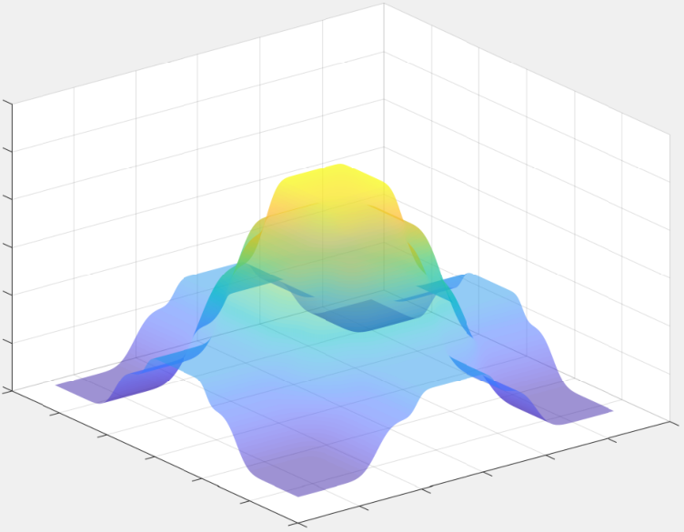
These three sampling distributions can be computed in the case of the Fourier-Haar transform. This is illustrated in Figure 2 for the 1D structured-sparsity pattern described in Figure 3(a). One can clearly see in Figure 2 that a certain prior on the sparsity structure in this case inclines the sensing in the low frequency domain. Reconstruction results are shown in Figure 3(b). For the same amount of measurements, the sampling strategy minimizing the bound on proposed in this paper is outperforming the standard CS strategy taking only into account the global coherence. In this setting, sampling according to improves the reconstruction quality compared to the -based strategy.
| (a) | (b) | (c) |
 |
 |
 |
| (d) | (e) | (f) |
| (a) | (b) |
5.2 Sensing vertical (or horizontal) lines in MRI
We extend the analysis of Section 5 from the one-dimensional to the two-dimensional framework, leading a more realistic model for the MRI problem.
Let for some and denote the one-dimensional Fourier-Haar transform introduced in Section 5.1 as . Then, we define the two-dimensional Fourier-Haar transform as
where denotes the Kronecker product. The splitting of the wavelet multi-index space and of the Fourier frequency space into subbands is carried out by tensorizing the one-dimensional splitting presented in Section 5.1. Namely, we consider subbands defined, for , as
Moreover, we will represent the image wavelet coefficients as a vector or, equivalently, as a matrix , such that , where is the vectorization operator that stacks the columns of a matrix atop, i.e., . Within this multi-level framework, we consider the following generalization of sparsity in levels.
Definition 5.1.
Let and be such that . Then, given , we define the following sparsities in levels for the vector :
| (54) |
where represents the set corresponding to the -th horizontal line or row of the wavelet multi-index space (see Figure 4).
The sparsities in levels are intrinsically anisotropic. According to this definition, the wavelet coefficients restricted to the vertical subband and to a generic row can be at most -sparse.
Equipped with this notion of structured sparsity, we consider measurements corresponding to vertical lines in the frequency space. This sensing strategy models MRI acquisition in a more realistic way than isolated Fourier measurements and corresponds to the setting (i) in Section 2.3. Specifically, we partition the set of rows of the matrix into blocks of size defined for as
where denotes the -th row of . Drawing the block corresponds to sampling along the vertical line in the frequency space.
In this setting, the analysis based on the quantity leads to the following result.
Corollary 5.2.
Let be the two-dimensional Fourier-Haar transform and consider the splitting of the Haar and of the Fourier spaces into subbands as defined above. Fix . Suppose that is an -sparse vector with random signs and associated structured sparsities in levels . Then, the same recovery guarantees of Theorem 3.6 hold with probability at least by drawing vertical lines according to the probability distribution defined as
with a number of drawn vertical lines of the order
| (55) |
In particular, the probability distribution is constant on each frequency subband .
The proof of this results is given in Appendix F.3. Corollary 5.2 meets the results of [BBW17, Corollary 4.10]: the bounds on the number of blocks of measurements are of the same order. Nevertheless, note that Corollary 5.2 requires an additional assumption on the sign randomness. Moreover, recall that Theorem 3.6 also ensures stable and robust recovery.
We can improve this result by analyzing the quantity .
Corollary 5.3.
Let be the two-dimensional Fourier-Haar transform and consider the splitting of the Haar and of the Fourier spaces into subbands as defined above. Fix . Suppose that is an -sparse vector with random signs and associated structured sparsities . If
then, the same recovery guarantees of Theorem 3.10 hold with probability at least by drawing vertical lines according to the probability distribution defined as
with a number of drawn vertical lines of the order
| (56) |
In particular, the probability distribution is constant on each frequency subband .
Note that the bound (56) improves Corollary 5.2 by attenuating the interference between different subbands sparsities.
Remark 5.4.
Results analogous to those presented in this Section hold when sampling horizontal lines in the Fourier space, up to replacing the structured sparsities in Definition 5.1 with
where is the -th vertical line of the wavelet multi-index space. In this case, sampling along the -th horizontal line corresponds to draw a block . The proofs in Appendix F.3 can be easily adapted to this setting by interchanging the role of rows and columns in the Haar and in the Fourier multi-index spaces, respectively (or, equivalently, by switching the order of tensorization).
Remark 5.5.
There is a mismatch between the notation adopted here and in [BBW17], where the role of rows and columns in the Haar and Fourier spaces is switched. As a result, horizontal Fourier sampling and structured sparsities in [BBW17] correspond to vertical Fourier sampling and structured sparsities , respectively, in our framework. Although choosing one of these two conventions might be considered just a matter of taste, we have changed notation in order to adhere to the way the two-dimensional Fourier transform is performed by the Matlab® command fft2. In our setting, fully-sampled measurements correspond to , where and . In particular, the block measurement corresponds to the -th column (or vertical line) of the matrix .
5.3 Adaptive sampling for function approximation
In this section, we examine the problem of approximating a function from random pointwise samples using standard sparsity with respect to Legendre polynomials [ABW17, CDTW17, RW12]. In particular, we will see how the theoretical results shown in this paper can be employed to construct effective adaptive sampling strategies. For the sake of simplicity, we will focus on the one-dimensional case, although the strategies presented here can be generalized to multiple dimensions.
Adaptive sampling strategies
Let and let be the family of Legendre orthogonal polynomials normalized such that . We aim at approximating as a sparse expansion of Legendre polynomials from a fixed budget of adaptively chosen pointwise samples.
In order to put ourselves in the framework of subsampled isometries, we consider the family of Gauss-Legendre quadrature points on and their respective quadrature weights (we recall that are the roots of the polynomial and the weights satisfy ). The resulting quadrature formula is exact on polynomials of degree less than or equal to . In particular, the matrix , defined as
| (57) |
is orthogonal. Based on the theory presented in this paper, we consider two adaptive sampling strategies based on successive approximations of the support via minimization. We refer to these strategies as (Adapt I) and (Adapt II). They are outlined in Algorithm 1 and described below.
Let us fix a target sparsity level and two numbers such that . Both procedures draw samples times, resulting in a total of samples. At each iteration, we compute an approximation to the function based on partial support information and we update the sampling measure accordingly. In particular, in the -th iteration, (Adapt I) updates the sampling measure based on the support corresponding to the entries of the -th approximation with largest magnitude. On the other hand, (Adapt II) updates the measure by taking advantage of the entries of the -th approximation having largest magnitude. This difference corresponds to line 5 of Algorithm 1.
Inputs: ,
Output:
Adaptive vs. nonadaptive sampling.
In order to evaluate the performance of adaptive sampling, we compare the following five sampling strategies:
- (Adapt I)
-
Adaptive sampling with fixed support size;
- (Adapt II)
-
Adaptive sampling with increasing support size;
- (Unif I)
-
Random sampling from the continuous uniform measure over ;
- (Unif II)
-
Uniform random sampling from ;
- (Cheby)
-
Random sampling from the continuous Chebyshev measure over ;
We fix and . For the strategies (Adapt I) and (Adapt II), we chose , , leading to a total number of adaptive measurements. We also fix the number of measurements as for the nonadaptive strategies (Unif I), (Unif II), and (Cheby). Moreover, we fix (using the spg_bp command of the SPGL1 Matlab® package to solve basis pursuit [vdBF07, vdBF08]). We run the following random experiment 100 times. For each run, we randomly generate a 5-sparse Legendre polynomial by selecting 5 indices uniformly at random form and by generating the respective coefficients independently at random according to the distribution . Then, we apply the five strategies to recover the resulting function from pointwise samples.
The results of this comparison are shown in Figure 6, where we plot the error of the approximate solution.
Adaptive sampling slightly outperforms nonadaptive sampling, but the gain is not substantial.
We also visualize the evolution of the sampling measure as a function of the iteration in Figure 7 for (Adapt I) and (Adapt II).


We notice that the strategy (Adapt I) does not refine the measure from the third iteration. On the contrary, the measure is updated at each iteration in the case of (Adapt II), which takes advantage of more support information.
Convergence of the adapted measure.
An interesting feature of the proposed adaptive sampling schemes is its capacity to converge to the optimal sampling measure. In the next experiment, we consider a random -sparse combination of the first Legendre polynomials. We compare the strategies (Adapt I) and (Adapt II) with , , and . We start sampling from a uniform grid on of points ( and are excluded). Moreover, we fix .
In Figure 8 we compare the measure for with the Chebyshev measure on the uniform grid (i.e., such that for every point of the uniform grid). We can see that for both (Adapt I) and (Adapt II) the adapted measure tends to approximate the Chebyshev measure. The convergence is more evident for the approach (Adapt II), where the approximate support gets larger and larger at each iteration.
| (Adapt I) | (Adapt II) |
|---|---|
A more quantitative convergence analysis is provided in Table 1, where we show the absolute error as a function of the iteration for both approaches. For (Adapt I), the error essentially stabilizes from the fourth iteration, whereas in the case of (Adapt II) it is monotonically decreasing. Comparing these data with Figure 8, we can see how (Adapt II) is able to correct the behavior of near the extrema to a substantial extent at each iteration. On the contrary, in the case of (Adapt I) the measure exhibits severe oscillations near .
| (Adapt I) | (Adapt II) | |
|---|---|---|
| 1.0102e-02 | 1.0102e-02 | |
| 4.4442e-03 | 6.3474e-03 | |
| 4.2014e-03 | 3.3659e-03 | |
| 3.8730e-03 | 2.7679e-03 | |
| 3.8730e-03 | 2.3916e-03 |
The convergence property of the proposed adaptive sampling strategies is particularly promising for high-dimensional approximation and, specifically, for the case of nontensorial domains, where the optimal sampling measure is not known a priori. However, this is beyond the scope of this paper and is left for future investigation.
6 Conclusions
We have derived novel oracle-type inequalities for the number of measurements needed to guarantee stable and robust recovery for compressed sensing in the noisy setting. Our analysis relies on a random sign assumption for the signal to be recovered and encompasses the frameworks of block-structured and isolated random measurements, in particular subsampled from a finite-dimensional isometry.
The proposed analysis reveals a direct link between the number of measurements and the support of the signal to be recovered. This allows one to derive optimal sampling strategies in order to minimize the number of measurements and that are tailored to particular sparsity structure in the signal support.
We have derived optimal sampling strategies in the case of (i) subsampling one-dimensional Fourier-Haar transform via isolated measurements combined with the sparsity in levels structure and (ii) subsampling the two-dimensional Fourier-Haar transform via block-structured measurements combined with anisotropic (horizontal or vertical) sparsity in levels. Finally, we have shown how to perform adaptive sampling for one-dimensional function approximation from pointwise data.
All these results are based on a random sign assumption; for future work, it would be worth devising alternative proof techniques in order to remove it. The analysis of the extra assumptions (32) and (33) involving and could be also refined: are they necessary conditions to obtain oracle-type results? As for applications, the polynomial approximation example reveals an adaptive sampling strategy that is worth deepening and extending to the multivariate case as well. Besides, one could adapt the oracle-type study to the case of weighted minimization which is of particular interest for polynomial approximation.
Acknowledgement
This work was supported by the Natural Sciences and Engineering Research Council of Canada [grant number 611675 to B.A. and S.B.]; and the Pacific Institute for the Mathematical Sciences (PIMS) [“PIMS Distinguished Visitor” program to C.B. and “PIMS Postdoctoral Training Centre in Stochastics” program to S.B].
The authors would like to thank Pierre Weiss for raising the optimal sampling concern and the anonymous referees for their insightful and constructive comments.
Appendix A Proof of the main results
A.1 Proof of Theorem 3.3
In order to prove that is the unique solution of (BP), one can use Fermat’s rule for (BP). Under injectivity of , this corresponds to the quest of a vector , called dual certificate, such that
A natural candidate for such a vector is the dual certificate with minimal -norm, i.e.
which trivially lies in the range of and satisfies . The second condition remains to be satisfied, as required by assumption (ii) of the following proposition.
Proposition A.1 ([FR13, Corollary 4.28]).
For with support , if
- (i)
is injective,
- (ii)
for all ,
then the vector is the unique solution of (BP) with .
By Lemma D.1, one gets the injectivity of with high probability. The rest of the proof is then dedicated to ensure (ii) of Proposition A.1. By a union bound, one can control the probability that (BP) fails to recover as follows:
where the last inequality is obtained using a Hoeffding-type bound (see [FR13, Corollary 7.21 and Corollary 8.10] for Rademacher and Steinhaus sequences, respectively). To control the second term, one can remark that for all
Using Lemma D.1, is bounded by for some with high probability. Using Lemma D.2, with high probability. Then, we set
The probability that (BP) fails is then bounded by
Note that by Lemma D.1 if
| (58) |
As for the last term , using Lemma D.2, choosing for some to be fixed later, one has if
| (59) |
where we have used that . Finally by setting , one has
Assuming that and choosing with leads to the previous inequality (notice that the constant 13 could be optimized in principle). Consequently, if
then .
A.2 Proof of Theorem 3.6
In order to ensure stable and robust recovery via (qBP), we take advantage of a result analogous to Proposition A.1, which hinges again on the concept of dual certificate. (Notice that in [FR13, Theorem 4.33] is assumed to be the set of largest absolute entries of , but an inspection of the proof reveals that can be an arbitrary subset of ).
Proposition A.2 ([FR13, Theorem 4.33]).
Let , , and with . For , with , assume that
| (60) |
and that there exists a vector with such that
If , then a minimizer of (qBP) satistfies
for some constants depending only on .
Using arguments analogous to the proof of Theorem 3.3, one can show that (60) holds with high probability. Therefore, using Proposition A.2, we choose the dual certificate to be with .
Since , for any , the condition is trivially satisfied (in particular, we can set ).
As for ensuring that with high probability, we have to slightly modify a part of the proof in the noiseless setting. First, let us observe that
For , using again a union bound and a Hoeffding-type inequality (see [FR13, Corollary 7.21 and Corollary 8.10] for Rademacher and Steinhaus sequences, respectively), one has
Now, analogously to the proof of Theorem 3.3, we fix
With these choices of parameters, conditions (58) and (59) suffice to guarantee that and , respectively. Moreover, since , if
then . Plugging this value of in (58) and (59), one gets the following conditions on the number of measurements:
Now, we have to find a suitable constant such that . Note that
since has full column rank. Moreover, observe that
Hence, one can choose , so that
which has been already controlled as .
Finally, in order to apply Proposition A.2, let us notice that since and .
This leads to the desired result.
A.3 Proof of Theorem 3.8
We will show a more general result, which will imply Theorem 3.8 as a corollary. In particular, in order to obtain Theorem 3.8 it will suffice to consider the partition formed by its singletons in Theorem A.3, i.e. .
Theorem A.3.
Let or be a vector supported on , such that forms a Rademacher or Steinhaus sequence. Let be the random sensing matrix defined in (9) with parameter and let , with . Then, there exist constants such that the following holds. For every , if
then, with probability at least , a minimizer of (qBP) satisfies
In particular, in the noiseless case (i.e., ), is exactly recovered via (BP) with probability at least and with constant .
For the sake of simplicity, let us address the case (the argument can be generalized to the case in the same spirit of Appendix A.2). Analogously to the proof of Theorem 3.3 in Appendix A.1, our aim is to find sufficient conditions such that
where . In the following, we show how to ensure that , for .
In order to control , let us consider a partition of and note that
where we have used that and where we have defined for each index of the partition. Now, combining the above inequality with Lemma D.1 and with a union bound over the elements of the partition , we obtain
Notice that introducing the partition allowed us to control by the quantity rather than . Simple algebraic manipulations show that the condition
| (61) |
is sufficient to have .
A.4 Proof of Theorem 3.10
The proof is analogous to that of Theorem 3.3. Therefore, we will employ the same notation as in Appendix A.1. By similar arguments, one has
for some and . Note that is controlled as before using Lemma D.1. In particular, if
| (62) |
Thus, let us suppose for the rest of the proof to choose
| (63) |
where is a constant that will be fixed later and where we are using . The slight modification in the proof compared to the one in Appendix A.1 appears in the control of . Indeed, using Lemma D.3, one has for some
Therefore, combining the above inequality with (63), fixing , and assuming that , one has
provided that
| (64) |
Condition on remains to be checked. In accordance with the previous computation, we set and if we choose , with , we obtain
Finally, we note that (64) holds true for, e.g., and . Therefore, conditions
ensure that (BP) exactly recovers with probability larger than .
Note that no effort was made in order to optimize the constants and , and the result in the noisy setting can be easily deduced from the noiseless one as in Appendix A.2.
Appendix B A discussion on stability
In Theorems 3.8, 3.9, and 3.10, we assume that the vector is exactly -sparse. However, it is possible to extend these results to the case of an arbitrary vector or such that is a random Rademacher or Steinhaus sequence. Indeed, in this case, if and the measurements are corrupted by noise such that , Proposition A.2 ensures a recovery guarantee of the form
This implies the stability of the recovery guarantees with respect to the standard sparsity model, in addition to its robustness to bounded noise. We now clarify in what sense this generalization of Theorems 3.8, 3.9, and 3.10 would still be of “oracle type”.
Let us go back to the proof of Proposition 3.1. We showed that the definition (28) of the oracle least-squares estimator is sufficient to have
| (65) |
Moreover, in view of Lemma D.1 condition (27) implies and . In order to make (65) a stable and robust recovery guarantee, we need to control the quantity . To achieve this, we observe that . Therefore, the condition
| (66) |
combined with (65), implies the following stable and robust recovery guarantee for the oracle least-squares estimator:
We conclude by observing that (66) is one of the hypotheses of Proposition A.2 (see (60)) and that it holds with probability at least under the assumptions on stated in any of the Theorems 3.8, 3.9, or 3.10 (recall the definition of in the corresponding proofs).
Appendix C Bernstein’s inequalities
In this section, we present two Bernstein-type inequalities employed in the proofs of Appendix D.
First, we present an extension of the vector Bernstein inequality [FR13, Theorem 8.45] in order to handle random vectors that are independent but not necessarily identically distributed. Then, we recall a Bernstein inequality for self-adjoint matrices, corresponding to [FR13, Corollary 8.15]. Note that both results are independent of the dimension of the random objects (vectors or matrices) involved.
Theorem C.1 (Vector Bernstein Inequality).
Consider a set of independent random vectors such that
and let such that
Then, for every , the following holds:
Proof.
Assume , consider , and let be a dense countable subset of . Define . Then, can be expressed as a supremum of an empirical process. Indeed,
where we have defined in the last step. Now, we verify the hypotheses needed to apply Talagrand’s inequality (see [FR13, Theorem 8.42]).
First, because the ’s are centered. Moreover, for every , almost surely and
Finally, Talagrand’s inequality yields
which is the desired result.
Theorem C.2 (Bernstein Inequality for self-adjoint matrices, [FR13, Corollary 8.15]).
Let be a finite sequence of independent, random, self-adjoint matrices such that and that a.s. for some constant independent of . Define
Then, for any , we have that
Appendix D Auxiliary lemmas
In this section, we show some deviation inequalities involving submatrices of the sensing matrix corresponding to the setting described in Section 2.3. In particular, the tail probabilities will be controlled by using the quantities , , and introduced in Definition 2.3, where .
The first auxiliary lemma controls the deviation of from the identity by means of the quantity .
Lemma D.1.
For every with and for every , the following holds
Proof.
Our objective is to apply Theorem C.2. Consider the splitting
Of course, . Moreover,
Now, observing that , we have
Being self-adjoint, we have
In order to estimate this term, we notice that
Now, observing that for every , we have
Therefore, . Now, we apply Theorem C.2 and we obtain
since , which concludes the proof.
The next two lemmas aim at controlling the growth of the absolute entries of in terms of the quantity .
Lemma D.2.
Let . Then, for every
Proof.
This proof is relies on Theorem C.1. Fix and consider . Note that since . Moreover,
Now, we verify the hypotheses of Theorem C.1 for the random vectors . Of course, . Moreover, recalling the definition of and of , we have
Therefore, we obtain
Then, using the Cauchy-Schwarz inequality, we estimate
where in the last step we used . Furthermore, using the independence of the ’s and their zero-mean property, we see that
Now, combining the above inequality with the following estimate
we obtain
We are now in a position to apply Theorem C.1. We have
A union bound over concludes the proof.
The next lemma is a refined version of Lemma D.2, involving the quantities and instead of . Indeed, it is worth recalling that .
Lemma D.3.
Let . Then, for every
Proof.
The proof relies on the Bernstein-type inequality in Theorem C.1. Fix and consider . Note that since . Moreover,
Now, we verify the hypotheses of Theorem C.1 for the random vectors . Of course, . Moreover, since
we obtain
Then, using the Cauchy-Schwarz inequality, we estimate
where in the last step we used . Furthermore, using the independence of the ’s, we see that
Now, combining the above inequality with the following estimate
we obtain
We are now in a position to apply Theorem C.1. We have
A union bound over concludes the proof.
Appendix E Proofs of Section 4
Propositions in Section 4 are direct consequences of the minimization of the bounds obtained on the number of measurements in Theorems of Section 3, given the following lemma.
Lemma E.1.
Given such that for all . Define for a probability distribution on , the following function:
Then, it holds that
and the unique minimizer of over discrete probability distributions is for all
Proof.
The proof is inspired by an intermediary result in [CCW13]. We give the proof here for completeness. Note that for , . For a probability distribution , there exists an index such that since both sum to 1. Then, .
Appendix F Proofs of Section 5
The appendix contains the proofs of the results stated in Section 5, regarding the application of the proposed analysis to the case of one-dimensional and two-dimensional Fourier-Haar setting.
F.1 Proof of Corollary 5.1
Let with be the Fourier-Haar transform and consider wavelet and frequency subbands and as illustrated in Section 5.1.
Recalling the local coherence estimate (46) from [AHR16, Lemma 1], one has for
where is the frequency level corresponding to index and where is a universal constant. Consequently, an estimate for is
Recalling Lemma E.1, the probability distribution minimizing the previous bound is such that for all
Since the size of the frequency subbands is , one can rewrite, for all
Therefore, since , we have
with . With such a choice of probability distribution , an estimate for can be derived as follows:
where we used that thanks to (46). Therefore Condition (33) is satisfied if
which, in turn, is equivalent to
Theorem 3.10 can be now applied, ensuring stable and robust recovery with probability with a required number of measurements
This concludes the proof of the corollary.
F.2 Proof of Corollary 5.2
The proof of Corollary 5.2 relies on the estimate of and on the choice of the corresponding optimal measure on the space of vertical lines. With a slight abuse of notation, here can be interpreted as a subset of or as a subset of , depending on whether vectorization is used or not. In order to estimate , we consider the term
Recalling that and that is an isometry, we obtain
Let us explicitly write
Then, we have
The local coherence bound (46) yields . We estimate
where is the -th vertical line of . Now, we observe that
Finally, using the above relation, the decomposition of into subbands , and resorting again to (46), we see that
This leads to the desired estimate of . Using Lemma E.1 we can then derive the corresponding optimal measure and conclude the proof.
F.3 Proof of Corollary 5.3
We divide the proof of Corollary 5.3 into two steps. First, we find the optimal sampling measure that minimizes and compute the corresponding . In the second step, we estimate and derive the extra condition on the structured sparsity of the signal.
Step 1: Estimate of and derivation of
As in the previous section, here can be interpreted as a subset of or as a subset of , depending on whether vectorization is used or not. Let us fix a frequency . Our first goal is to estimate the quantity . This will lead us to the optimal choice of .
First, we observe that . Now, let and be such that (recall that the vectorization operator stacks the columns of a matrix on top of each other). Taking into account the structure of and , and recalling that is an isometry, we have
Taking advantage of the decomposition of the wavelet multi-index space into tensor product subbands and recalling (46), we extend the previous chain of equalities as follows:
where is such that and is the local coherence of the Fourier-Haar transform defined in (46). Using the Cauchy-Schwarz inequality, rearranging the summation, and recalling Definition 5.1, we see that
Combining the above relations an using again (46) yields
where is the universal constant in (46). Using Lemma E.1 and recalling that , the optimal probability is, for all ,
This leads to
Step 2: Estimate of and conclusion
References
- [ABW17] Ben Adcock, Simone Brugiapaglia, and Clayton G. Webster. Compressed sensing approaches for polynomial approximation of high-dimensional functions. In Compressed Sensing and its Applications, pages 93–124. Springer, 2017.
- [AHPR17] Ben Adcock, Anders C. Hansen, Clarice Poon, and Bogdan Roman. Breaking the coherence barrier: A new theory for compressed sensing. In Forum of Mathematics, Sigma, volume 5. Cambridge University Press, 2017.
- [AHR14] Ben Adcock, Anders C. Hansen, and Bogdan Roman. The quest for optimal sampling: Computationally efficient, structure-exploiting measurements for compressed sensing. Book Chapter, Compressed Sensing and its Applications, Springer (to appear), arXiv preprint arXiv:1403.6540, 2014.
- [AHR16] Ben Adcock, Anders C. Hansen, and Bogdan Roman. A note on compressed sensing of structured sparse wavelet coefficients from subsampled fourier measurements. IEEE Signal Processing Letters, 23(5):732–736, 2016.
- [ALMT14] Dennis Amelunxen, Martin Lotz, Michael B McCoy, and Joel A. Tropp. Living on the edge: Phase transitions in convex programs with random data. Information and Inference: A Journal of the IMA, 3(3):224–294, 2014.
- [BBW14] Jérémie Bigot, Claire Boyer, and Pierre Weiss. An analysis of blocks sampling strategies in compressed sensing. arXiv preprint arXiv:1310.4393, 2014.
- [BBW17] Claire Boyer, Jérémie Bigot, and Pierre Weiss. Compressed sensing with structured sparsity and structured acquisition. Applied and Computational Harmonic Analysis, 2017.
- [CA17] Il Yong Chun and Ben Adcock. Compressed sensing and parallel acquisition. IEEE Transactions on Information Theory, 2017.
- [CCKW14] Nicolas Chauffert, Philippe Ciuciu, Jonas Kahn, and Pierre Weiss. Variable density sampling with continuous trajectories. SIAM Journal on Imaging Sciences, 7(4):1962–1992, 2014.
- [CCW13] Nicolas Chauffert, Philippe Ciuciu, and Pierre Weiss. Variable density compressed sensing in MRI. Theoretical vs heuristic sampling strategies. In Biomedical Imaging (ISBI), 2013 IEEE 10th International Symposium on, pages 298–301. IEEE, 2013.
- [CDTW17] Abdellah Chkifa, Nick Dexter, Hoang Tran, and Clayton G. Webster. Polynomial approximation via compressed sensing of high-dimensional functions on lower sets. Mathematics of Computation, 2017.
- [CP11] Emmanuel Candès and Yaniv Plan. A probabilistic and ripless theory of compressed sensing. Information Theory, IEEE Transactions on, 57(11):7235–7254, 2011.
- [CR07] Emmanuel Candès and Justin Romberg. Sparsity and incoherence in compressive sampling. Inverse problems, 23(3):969, 2007.
- [FR13] Simon Foucart and Holger Rauhut. A mathematical introduction to compressive sensing. Springer, 2013.
- [KW14] Felix Krahmer and Rachel Ward. Stable and robust sampling strategies for compressive imaging. IEEE transactions on image processing, 23(2):612–622, 2014.
- [LA17] Chen Li and Ben Adcock. Compressed sensing with local structure: uniform recovery guarantees for the sparsity in levels class. Appl. Comput. Harmon. Anal. (to appear), 2017.
- [LHZ+14] Li Liu, Yuntao He, Jianguo Zhang, Huayu Jia, and Jun Ma. Optimum linear array for aperture synthesis imaging based on redundant spacing calibration. Optical Engineering, 53(5):053109, 2014.
- [PVW11] Gilles Puy, Pierre Vandergheynst, and Yves Wiaux. On variable density compressive sampling. Signal Processing Letters, IEEE, 18(10):595–598, 2011.
- [QBGK10] Céline Quinsac, Adrian Basarab, Jean-Marc Girault, and Denis Kouamé. Compressed sensing of ultrasound images: Sampling of spatial and frequency domains. In Signal Processing Systems (SIPS), 2010 IEEE Workshop on, pages 231–236. IEEE, 2010.
- [RW12] Holger Rauhut and Rachel Ward. Sparse legendre expansions via -minimization. Journal of approximation theory, 164(5):517–533, 2012.
- [Tro15] Joel A. Tropp. Convex recovery of a structured signal from independent random linear measurements. In Sampling Theory, a Renaissance, pages 67–101. Springer, 2015.
- [vdBF07] Ewout van den Berg and Michael P. Friedlander. SPGL1: A solver for large-scale sparse reconstruction, June 2007. http://www.cs.ubc.ca/labs/scl/spgl1.
- [vdBF08] Ewout van den Berg and Michael P. Friedlander. Probing the pareto frontier for basis pursuit solutions. SIAM Journal on Scientific Computing, 31(2):890–912, 2008.
- [Wan00] Yi Wang. Description of parallel imaging in mri using multiple coils. Magnetic Resonance in Medicine, 44(3):495–499, 2000.