跳到论文正文
W Papers独立论文阅读器 arXiv:1806.03742 论文正文 计算阅读时间 · 0%
引用这篇论文根据当前论文元数据生成,正式投稿前建议核对。


License: arXiv.org perpetual non-exclusive license
arXiv:1806.03742v1 [math-ph] 10 Jun 2018

Dimer Model: Full Asymptotic Expansion of the Partition Function

Abstract.

We give a complete rigorous proof of the full asymptotic expansion of the partition function of the dimer model on a square lattice on a torus for general weights zh,zvz_{h},z_{v} of the dimer model and arbitrary dimensions of the lattice m,nm,n. We assume that mm is even and we show that the asymptotic expansion depends on the parity of nn. We review and extend the results of Ivashkevich, Izmailian, and Hu [6] on the full asymptotic expansion of the partition function of the dimer model, and we give a rigorous estimate of the error term in the asymptotic expansion of the partition function.

Pavel Bleher** * pbleher@iupui.edu, Brad Elwood†† † bradelwood@gmail.com, Dražen Petrovi懇 ‡ petrovic.drazen@gmail.com

Indiana University-Purdue University Indianapolis

August 24, 2026

The first author is supported in part by the National Science Foundation (NSF) Grant DMS-1565602.

1. Introduction

1.1. Dimer Model on a Square Lattice

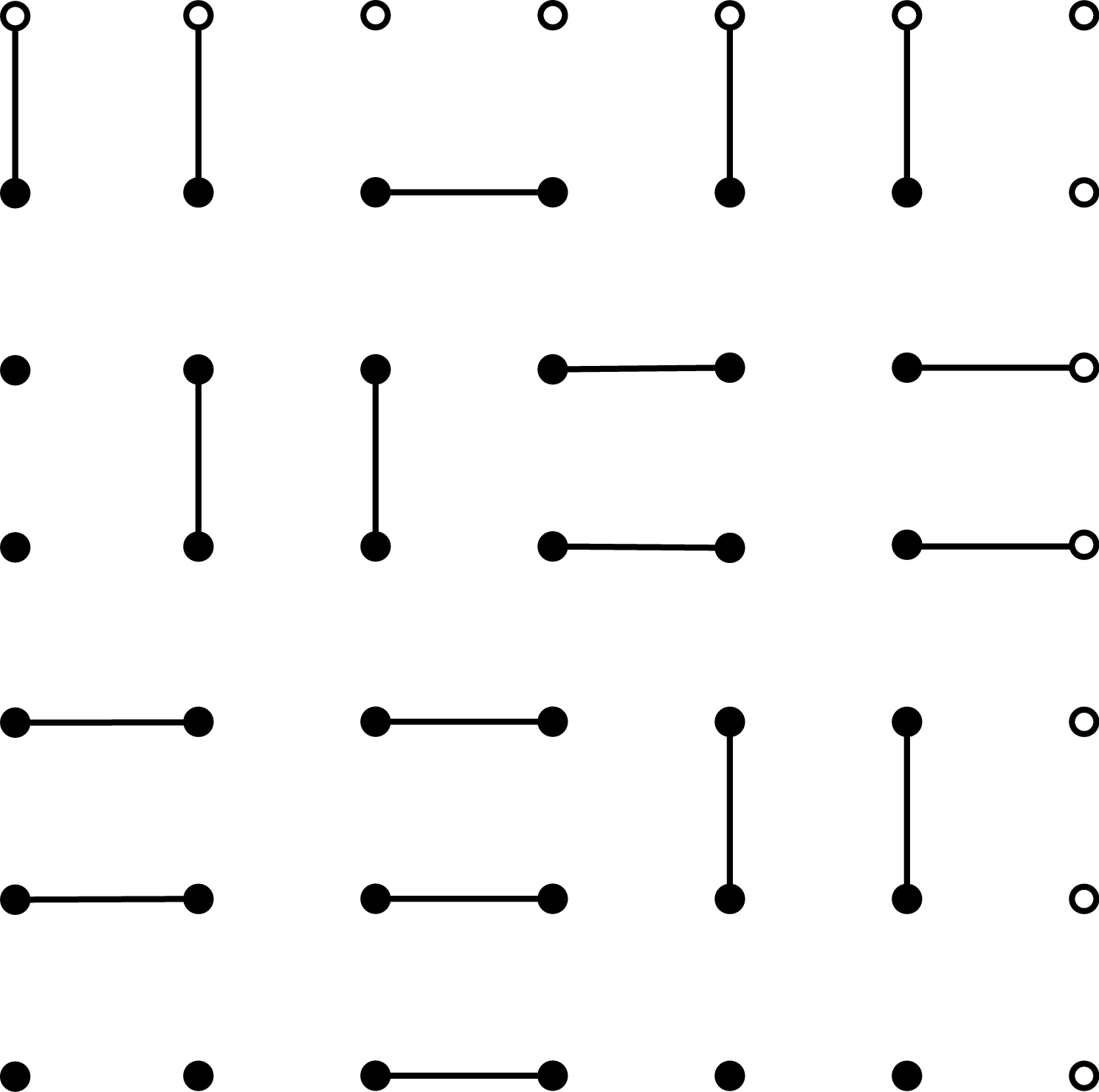
We consider the dimer model on a square lattice Γm,n=(Vm,n,Em,n)\Gamma_{m,n}=(V_{m,n},E_{m,n}) on the torus ℤm×ℤn=ℤ2/(m​ℤ×n​ℤ){\mathbb{Z}}_{m}\times{\mathbb{Z}}_{n}={\mathbb{Z}}^{2}/(m{\mathbb{Z}}\times n{\mathbb{Z}}) (periodic boundary conditions), where Vm,nV_{m,n} and Em,nE_{m,n} are the sets of vertices and edges of Γm,n,\Gamma_{m,n}, respectively. A dimer on Γm,n\Gamma_{m,n} is a set of two neighboring vertices ⟨x,y⟩\langle x,y\rangle connected by an edge. A dimer configuration σ\sigma on Γm,n\Gamma_{m,n} is a set of dimers σ={⟨xi,yi⟩,i=1,…,m​n2}\sigma=\{\langle x_{i},y_{i}\rangle,\;i=1,\ldots,\frac{mn}{2}\} which cover Vm,nV_{m,n} without overlapping. An example of a dimer configuration is shown in Fig. 1. An obvious necessary condition for a configuration to exist is that at least one of m,nm,n is even, and so we assume that mm is even, m=2​m0m=2m_{0}.

Refer to caption
Figure 1. Example of a dimer configuration on a square 6×66\times 6 lattice on the torus.

To define a weight of a dimer configuration, we split the full set of dimers in a configuration σ\sigma into two classes: horizontal and vertical, with respective weights zh,zv>0.z_{h},z_{v}>0. If we denote the total number of horizontal and vertical dimers in σ\sigma by Nh​(σ)N_{h}(\sigma) and Nv​(σ),N_{v}(\sigma), respectively, then the dimer configuration weight is

w⁡(σ)=∏i=1m​n2w⁡(xi,yi)=zhNh​(σ)​zvNv​(σ),w(\sigma)=\prod_{i=1}^{\frac{mn}{2}}w(x_{i},y_{i})=z_{h}^{N_{h}(\sigma)}z_{v}^{N_{v}(\sigma)}, (1.1)

where w⁡(xi,yi)w(x_{i},y_{i}) denotes the weight of the dimer ⟨xi,yi⟩∈σ\langle x_{i},y_{i}\rangle\in\sigma. We denote by Σm,n\Sigma_{m,n} the set of all dimer configurations on Γm,n\Gamma_{m,n}. The partition function of the dimer model is given by

Z=∑σ∈Σm,nw⁡(σ).Z=\sum_{\sigma\in\Sigma_{m,n}}w(\sigma). (1.2)

Notice that if all the weights are set equal to one, then ZZ simply counts the number of dimer configurations, or perfect matchings, on Γm,n\Gamma_{m,n}.

Our goal is to evaluate the full asymptotic series expansion of the partition function ZZ as m,n→∞m,n\to\infty. The free energy of the dimer model on the square lattice was obtained in the papers of Kasteleyn [8] and Temperley and Fisher [16]. Our work is based on the Kasteleyn’s expression of the partition function ZZ on a torus as a linear combination of 4 Pfaffians developed in the works [8], [9], [10] (see also the works of Galluccio and Loebl [5], Tesler [17], and Cimasoni and Reshetikhin [3]). The constant term in the asymptotic of the partition function was obtained by Ferdinand [4] (see also the work of Kenyon, Sun and Wilson [11]).

The asymptotic expansion of the partition function on a torus was developed by Ivashkevich, Izmailian, and Hu [6] and our calculations use their ideas. Ivashkevich, Izmailian, and Hu considered the case when zh=zvz_{h}=z_{v} and nn is even. In the present work we extend their calculations to arbitrary weights zh,zvz_{h},z_{v} and to odd nn. It is worth noticing that the asymptotic expansions for even and odd values of nn are different. We give a complete rigorous proof of the asymptotic expansion of the partition function, with an estimate of the error term. The asymptotic expansion of the partition function is expressed in terms of the classical Jacobi theta functions, Dedekind eta function, and Kronecker double series. The work [6] has been further extended by Izmailian, Oganesyan, and Hu [7] to the dimer model on a square lattice with various boundary conditions for both even and odd nn. Our result for the dimer model on a torus coincides with the one in [7] for even nn, and for odd nn it coincides except for the value of the elliptic nome in formula (2.14) below. The difference in the value of the elliptic nome for even and odd nn is explained after formula (5.6) in Section 5 below.

It follows from (1.1), (1.2) that the partition function ZZ is a homogeneous polynomial of the variables zh,zvz_{h},z_{v}, and it can be written as

Z⁡(zh,zv)=∑σ∈Σm,nzhNh​(σ)​zvNv​(σ)=zhm​n2​Z​(1,ζ),Z(z_{h},z_{v})=\sum_{\sigma\in\Sigma_{m,n}}z_{h}^{N_{h}(\sigma)}z_{v}^{N_{v}(\sigma)}=z_{h}^{\frac{mn}{2}}Z(1,\zeta), (1.3)

where

ζ=zvzh>0,\zeta=\frac{z_{v}}{z_{h}}>0, (1.4)

so without loss of generality we may assume that

zh=1,zv=ζ,z_{h}=1,\quad z_{v}=\zeta, (1.5)

and we will evaluate the full asymptotic series expansion of the partition function Z⁡(1,ζ)Z(1,\zeta) as m,n→∞m,n\to\infty.

To formulate our main result we have to introduce and remind some special functions and operators.

1.2. Function g⁡(x)g(x)

Introduce the function

g⁡(x)=ln⁡(ζ​sin⁡(π​x)+1+ζ2​sin2⁡(π​x)),g(x)=\ln\left(\zeta\sin(\pi x)+\sqrt{1+\zeta^{2}\sin^{2}(\pi x)}\right), (1.6)

where ζ>0\zeta>0 is defined in (1.4). Observe that g⁡(x)g(x) has the following properties:

  1. (1)

    g⁡(−x)=−g⁡(x),g(-x)=-g(x),

  2. (2)

    g⁡(x+1)=−g⁡(x),g(x+1)=-g(x),

  3. (3)

    g⁡(x)g(x) is real analytic on [0,1][0,1] and

    g⁡(x)=∑p=0∞g2​p+1​x2​p+1,g\left(x\right)=\sum_{p=0}^{\infty}g_{2p+1}x^{2p+1}, (1.7)

    where

    g1=πζ,g3=−π3​ζ​(ζ2+1)6,g5=π5​ζ​(ζ2+1)​(9​ζ2+1)120,….g_{1}=\pi\zeta,\quad g_{3}=-\frac{\pi^{3}\zeta(\zeta^{2}+1)}{6}\,,\quad g_{5}=\frac{\pi^{5}\zeta(\zeta^{2}+1)(9\zeta^{2}+1)}{120}\,,\;\ldots. (1.8)
  4. (4)

    g⁡(x)≥C0​xg(x)\geq C_{0}x on the segment 0≤x≤120\leq x\leq\frac{1}{2}\,, with some C0>0C_{0}>0.

The constant C0C_{0} in the latter inequality can depend on ζ\zeta. In what follows we assume that ζ\zeta is fixed and we do not indicate the dependence of various constants CkC_{k} on ζ\zeta. Unless otherwise is stated, the constants CkC_{k} can be different in different inequalities.

Observe that since g⁡(x)g(x) is analytic at x=0x=0, we have that

|g2​p+1|≤C​ξp,\left|g_{2p+1}\right|\leq C\xi^{p}, (1.9)

with some C,ξ>0C,\xi>0.

1.3. Differential Operator Δp\Delta_{p}

Let 𝒮p\mathcal{S}_{p} be the set of collections of positive integers
(p1,…,pr,q1,…,qr)(p_{1},\ldots,p_{r};q_{1},\ldots,q_{r}), 1≤r≤p1\leq r\leq p, such that

𝒮p={(p1,…,pr;q1,…,qr)| 0<p1<…<pr;p1q1+…+prqr=p}.\displaystyle\mathcal{S}_{p}=\left\{(p_{1},\ldots,p_{r};q_{1},\ldots,q_{r})\;\big|\;0<p_{1}<\ldots<p_{r};\;p_{1}q_{1}+\ldots+p_{r}q_{r}=p\right\}. (1.10)

Introduce the differential operator

Δp=∑𝒮p(g2​p1+1)q1​…​(g2​pr+1)qrq1!​…​qr!dqd​λq,q=q1+…+qr−1.\displaystyle\Delta_{p}=\sum_{\mathcal{S}_{p}}\frac{(g_{2p_{1}+1})^{q_{1}}\ldots(g_{2p_{r}+1})^{q_{r}}}{q_{1}!\ldots q_{r}!}\,\frac{d^{q}}{d\lambda^{q}}\,,\quad q=q_{1}+\ldots+q_{r}-1\,. (1.11)

Observe that

Δ1=g3,Δ2=g322dd​λ+g5,Δ3=g333!d2d​λ2+g3g5dd​λ+g7,….\Delta_{1}=g_{3},\quad\Delta_{2}=\frac{g^{2}_{3}}{2}\frac{d}{d\lambda}+g_{5},\quad\Delta_{3}=\frac{g_{3}^{3}}{3!}\frac{d^{2}}{d\lambda^{2}}+g_{3}g_{5}\frac{d}{d\lambda}+g_{7},\quad\ldots\ . (1.12)

1.4. Kronecker’s Double Series

The Kronecker double series of order pp with parameters α,β\alpha,\beta is defined as

Kα,βp(τ)=−p!(−2​π​i)p∑(j,k)≠(0,0)e⁡(j​α+k​β)(k+τ​j)p,\displaystyle K^{\alpha,\beta}_{p}(\tau)=-\frac{p!}{(-2\pi i)^{p}}\sum_{(j,k)\not=(0,0)}\frac{e(j\alpha+k\beta)}{(k+\tau j)^{p}}\,, (1.13)

where

e⁡(x)=e−2​π​i​x.\displaystyle e(x)=e^{-2\pi ix}. (1.14)

We will use the following Kronecker double series with parameters (α,β)=(12,12),(0,12),(12,0)(\alpha,\beta)=(\frac{1}{2},\frac{1}{2}),(0,\frac{1}{2}),(\frac{1}{2},0), respectively:

Kp12,12​(τ)=\displaystyle K^{\frac{1}{2},\frac{1}{2}}_{p}(\tau)= −p!(−2​π​i)p∑(j,k)≠(0,0)(−1)j+k(k+τ​j)p,\displaystyle-\frac{p!}{(-2\pi i)^{p}}\sum_{(j,k)\not=(0,0)}\frac{(-1)^{j+k}}{(k+\tau j)^{p}}, (1.15)
Kp0,12​(τ)=\displaystyle K^{0,\frac{1}{2}}_{p}(\tau)= −p!(−2​π​i)p∑(j,k)≠(0,0)(−1)k(k+τ​j)p,\displaystyle-\frac{p!}{(-2\pi i)^{p}}\sum_{(j,k)\not=(0,0)}\frac{(-1)^{k}}{(k+\tau j)^{p}},
Kp12,0​(τ)=\displaystyle K^{\frac{1}{2},0}_{p}(\tau)= −p!(−2​π​i)p∑(j,k)≠(0,0)(−1)j(k+τ​j)p.\displaystyle-\frac{p!}{(-2\pi i)^{p}}\sum_{(j,k)\not=(0,0)}\frac{(-1)^{j}}{(k+\tau j)^{p}}\,.

We will use it for τ\tau pure imaginary and p≥4p\geq 4. Then the double series are absolutely convergent.

1.5. Dedekind Eta Function

The Dedekind eta function is defined as

η=η⁡(τ)=eπ​i​τ12​∏k=1∞(1−e2​π​i​τ​k)=q112​∏k=1∞(1−q2​k),\displaystyle\eta=\eta(\tau)=e^{\frac{\pi i\tau}{12}}\prod_{k=1}^{\infty}\left(1-e^{2\pi i\tau k}\right)=q^{\frac{1}{12}}\prod_{k=1}^{\infty}\left(1-q^{2k}\right), (1.16)

where

q=eπ​i​τq=e^{\pi i\tau} (1.17)

is the elliptic nome.

1.6. Jacobi Theta Functions

There are four Jacobi theta functions:

θ1​(z,q)\displaystyle\theta_{1}(z,q) =2​∑k=0∞(−1)k​q(k+12)2​sin⁡((2​k+1)​z),\displaystyle=2\sum_{k=0}^{\infty}(-1)^{k}q^{\left(k+\frac{1}{2}\right)^{2}}\sin\big((2k+1)z\big), (1.18)
θ2​(z,q)\displaystyle\theta_{2}(z,q) =2​∑k=0∞q(k+12)2​cos⁡((2​k+1)​z),\displaystyle=2\sum_{k=0}^{\infty}q^{\left(k+\frac{1}{2}\right)^{2}}\cos\big((2k+1)z\big),
θ3​(z,q)\displaystyle\theta_{3}(z,q) =1+2​∑k=1∞qk2​cos⁡(2​k​z),\displaystyle=1+2\sum_{k=1}^{\infty}q^{k^{2}}\cos(2kz),
θ4​(z,q)\displaystyle\theta_{4}(z,q) =1+2​∑k=1∞(−1)k​qk2​cos⁡(2​k​z),\displaystyle=1+2\sum_{k=1}^{\infty}(-1)^{k}q^{k^{2}}\cos(2kz),

where q=eπ​i​τq=e^{\pi i\tau} is elliptic nome.

We have the following identities (see, e.g., [18]):

θ2=θ2​(0,q)=2​η2​(2​τ)η⁡(τ),\displaystyle\theta_{2}=\theta_{2}(0,q)=\frac{2\eta^{2}(2\tau)}{\eta(\tau)}\,, (1.19)
θ3=θ3​(0,q)=η5​(τ)η2​(2​τ)​η2​(τ2),\displaystyle\theta_{3}=\theta_{3}(0,q)=\frac{\eta^{5}(\tau)}{\eta^{2}(2\tau)\eta^{2}(\frac{\tau}{2})}\,,
θ4=θ4​(0,q)=η2​(τ2)η⁡(τ).\displaystyle\theta_{4}=\theta_{4}(0,q)=\frac{\eta^{2}(\frac{\tau}{2})}{\eta(\tau)}\,.

Also (see, e.g., [6]),

K40,12​(τ)\displaystyle K_{4}^{0,\frac{1}{2}}(\tau) =130​(78​θ28−θ34​θ44),\displaystyle=\frac{1}{30}\left(\frac{7}{8}\theta_{2}^{8}-\theta_{3}^{4}\theta_{4}^{4}\right)\,, (1.20)
K412,0​(τ)\displaystyle K_{4}^{\frac{1}{2},0}(\tau) =130​(78​θ48−θ24​θ34),\displaystyle=\frac{1}{30}\left(\frac{7}{8}\theta_{4}^{8}-\theta_{2}^{4}\theta_{3}^{4}\right)\,,
K412,12​(τ)\displaystyle K_{4}^{\frac{1}{2},\frac{1}{2}}(\tau) =130​(78​θ38+θ24​θ44).\displaystyle=\frac{1}{30}\left(\frac{7}{8}\theta_{3}^{8}+\theta_{2}^{4}\theta_{4}^{4}\right)\,.

2. Main Result: Full Asymptotic Expansion of the Dimer Model Partition Function

2.1. Pfaffians

We would like to evaluate the asymptotic expansion of the dimer model partition function ZZ on the square lattice, Γm,n\Gamma_{m,n}, of dimensions m×nm\times n, with periodic boundary conditions where m,n→∞m,n\to\infty under the assumption that there exist positive constants C2>C1C_{2}>C_{1} such that

C1≤mn≤C2.C_{1}\leq\frac{m}{n}\leq C_{2}. (2.1)

As shown by Kasteleyn [8, 9, 10], the partition function ZZ can be written in terms of four Pfaffians as

Z=12​(−Pf⁡A1+Pf⁡A2+Pf⁡A3+Pf⁡A4),Z=\frac{1}{2}\left(-{\operatorname{Pf}\,}A_{1}+{\operatorname{Pf}\,}A_{2}+{\operatorname{Pf}\,}A_{3}+{\operatorname{Pf}\,}A_{4}\right), (2.2)

where A1,A2,A3,A4A_{1},A_{2},A_{3},A_{4} are the antisymmetric Kasteleyn matrices with periodic-periodic, periodic-antiperiodic, antiperiodic-periodic, and antiperiodic-antiperiodic boundary conditions, respectively. Their determinants are given by the double product formulae as

detAi=∏j=0m2−1∏k=0n−1[4​(sin2⁡2​π​(j+αi)m+ζ2​sin2⁡2​π​(k+βi)n)],\displaystyle\det A_{i}=\prod_{j=0}^{\frac{m}{2}-1}\prod_{k=0}^{n-1}\left[4\left(\sin^{2}\frac{2\pi(j+\alpha_{i})}{m}+\zeta^{2}\sin^{2}\frac{2\pi(k+\beta_{i})}{n}\right)\right], (2.3)

with

(α1,β1)=(0,0),(α2,β2)=(0,1/2),(α3,β3)=(1/2,0),(α4,β4)=(1/2,1/2).\displaystyle(\alpha_{1},\beta_{1})=(0,0),\quad(\alpha_{2},\beta_{2})=(0,1/2),\quad(\alpha_{3},\beta_{3})=(1/2,0),\quad(\alpha_{4},\beta_{4})=(1/2,1/2). (2.4)

These double product formulae are obtained by diagonalizing the matrices AiA_{i} (see [8, 13, 14]). The Pfaffian of a square antisymmetric matrix AA is related to its determinant through the classical identity:

(Pf⁡A)2=detA.({\operatorname{Pf}\,}A)^{2}=\det A. (2.5)

Observe that detA1=0\det A_{1}=0 due to the factor j=k=0j=k=0 in (2.3), hence

Pf⁡A1=0,{\operatorname{Pf}\,}A_{1}=0, (2.6)

and for odd nn, detA2=0\det A_{2}=0, due to the factor j=0j=0, k=n−12k=\frac{n-1}{2}\,, hence

Pf⁡A2=0,if n is odd.{\operatorname{Pf}\,}A_{2}=0,\quad\textrm{if $n$ is odd.} (2.7)

In addition,

Pf⁡A3=Pf⁡A4,if n is odd{\operatorname{Pf}\,}A_{3}={\operatorname{Pf}\,}A_{4},\quad\textrm{if $n$ is odd} (2.8)

(see [2]). As shown in [11],[2],

Pf⁡A2>0,if n is even,\displaystyle{\displaystyle\operatorname{Pf}\,}A_{2}>0,\quad\textrm{if $n$ is even}, (2.9)
PfA3>0,PfA4>0for all n,\displaystyle{\displaystyle\operatorname{Pf}\,}A_{3}>0,\quad{\operatorname{Pf}\,}A_{4}>0\quad\textrm{for all $n$},

hence from (2.3) we obtain that

Pf⁡Ai=∏j=0m2−1∏k=0n−1[4​(sin2⁡2​π​(j+αi)m+ζ2​sin2⁡2​π​(k+βi)n)]1/2.\displaystyle{\displaystyle\operatorname{Pf}\,}A_{i}=\prod_{j=0}^{\frac{m}{2}-1}\prod_{k=0}^{n-1}\left[4\left(\sin^{2}\frac{2\pi(j+\alpha_{i})}{m}+\zeta^{2}\sin^{2}\frac{2\pi(k+\beta_{i})}{n}\right)\right]^{1/2}. (2.10)

Combining (2.2) with (2.6), (2.7), (2.8), we obtain that

Z\displaystyle Z =12​(Pf⁡A2+Pf⁡A3+Pf⁡A4),if n is even,\displaystyle=\frac{1}{2}\left({\operatorname{Pf}\,}A_{2}+{\operatorname{Pf}\,}A_{3}+{\operatorname{Pf}\,}A_{4}\right),\quad\textrm{if $n$ is even}, (2.11)
Z\displaystyle Z =Pf⁡A3,if n is odd.\displaystyle={\operatorname{Pf}\,}A_{3},\quad\textrm{if $n$ is odd}.

2.2. Main Result

Before stating the main theorem, let us introduce some additional notations. Denote

S=m​n,ν=mn.S=mn,\qquad\nu=\frac{m}{n}\,. (2.12)

We set

τ={i​ζ​ν,if n is even,i​ζ​ν2,if n is odd,\tau=\begin{cases}i\zeta\nu,&\text{if $n$ is even,}\\ \frac{i\zeta\nu}{2},&\text{if $n$ is odd,}\end{cases} (2.13)

so that the elliptic nome is equal to

q=eπ​i​τ={e−π​ζ​ν,if n is even,e−π​ζ​ν2,if n is odd.q=e^{\pi i\tau}=\begin{cases}e^{-\pi\zeta\nu},&\text{if $n$ is even,}\\ e^{\frac{-\pi\zeta\nu}{2}},&\text{if $n$ is odd.}\end{cases} (2.14)

For brevity we also denote

η=η(τ),θk=θk(0,q),k=2,3,4,\eta=\eta(\tau),\qquad\theta_{k}=\theta_{k}(0,q),\quad k=2,3,4, (2.15)

where η⁡(τ)\eta(\tau) is the Dedekind eta function, and θk​(z,q)\theta_{k}(z,q) are the Jacobi theta functions. The main result is the following asymptotic expansion of the partition function ZZ in powers of S−1S^{-1}, derived by Ivashkevich et al. in [6] in the case ζ=1\zeta=1 and nn is even. We give a complete rigorous proof of the asymptotic expansion for any ζ>0\zeta>0 and for nn both even and odd.

Theorem 2.1.

If nn is even, then as m,n→∞m,n\to\infty under condition (2.1), we have that

Z=eS​F​(C(2)​eR(2)+C(3)​eR(3)+C(4)​eR(4)),\displaystyle Z=e^{SF}\left(C^{(2)}e^{R^{(2)}}+C^{(3)}e^{R^{(3)}}+C^{(4)}e^{R^{(4)}}\right), (2.16)

where

F=1π​∫0ζarctan⁡xx​dx,\displaystyle F=\frac{1}{\pi}\int\limits\limits_{0}^{\zeta}\frac{\arctan x}{x}\,dx, (2.17)
C(2)=θ422​η2,C(3)=θ222​η2,C(4)=θ322​η2,\displaystyle C^{(2)}=\frac{\theta_{4}^{2}}{2\eta^{2}},\quad C^{(3)}=\frac{\theta_{2}^{2}}{2\eta^{2}},\quad C^{(4)}=\frac{\theta_{3}^{2}}{2\eta^{2}}, (2.18)

and R(j)R^{(j)}, j=2,3,4j=2,3,4, admit the asymptotic expansions

R(j)∼∑p=1∞Rp(j)Sp,j=2,3,4,\displaystyle R^{(j)}\sim\sum_{p=1}^{\infty}\frac{R_{p}^{(j)}}{S^{p}}\,,\quad j=2,3,4, (2.19)

with

Rp(j)=−22​p+1​νp+1p+1​Δp​[K2​p+2βj,αj​(i​ν​λπ)]|λ=π​ζ,\displaystyle R_{p}^{(j)}=-\frac{2^{2p+1}\nu^{p+1}}{p+1}\,\Delta_{p}\left[K_{2p+2}^{\beta_{j},\alpha_{j}}\left(\frac{i\nu\lambda}{\pi}\right)\right]\bigg|_{\lambda=\pi\zeta}\,, (2.20)

where αj,βj\alpha_{j},\beta_{j} are defined in (2.4). In particular, by (1.12) and (1.20),

R1(2)=−2​ν2​g315(78θ48−θ24θ34),R1(3)=−2​ν2​g315(78θ28−θ34θ44),\displaystyle R_{1}^{(2)}=-\frac{2\nu^{2}g_{3}}{15}\bigg(\frac{7}{8}\theta_{4}^{8}-\theta_{2}^{4}\theta_{3}^{4}\bigg)\,,\quad R_{1}^{(3)}=-\frac{2\nu^{2}g_{3}}{15}\bigg(\frac{7}{8}\theta_{2}^{8}-\theta_{3}^{4}\theta_{4}^{4}\bigg)\,, (2.21)
R1(4)=−2​ν2​g315​(78​θ38+θ24​θ44).\displaystyle R_{1}^{(4)}=-\frac{2\nu^{2}g_{3}}{15}\bigg(\frac{7}{8}\theta_{3}^{8}+\theta_{2}^{4}\theta_{4}^{4}\bigg)\,.

Furthermore, if nn is odd, then as m,n→∞m,n\to\infty under condition (2.1), we have that

Z=C​eS​F+R,\displaystyle Z=Ce^{SF+R}, (2.22)

where FF is given in (2.17),

C=θ2η,\displaystyle C=\frac{\theta_{2}}{\eta}, (2.23)

and RR admits the asymptotic expansions

R∼∑p=1∞RpSp,\displaystyle R\sim\sum_{p=1}^{\infty}\frac{R_{p}}{S^{p}}\,, (2.24)

with

Rp=−νp+1p+1​Δp​[K2​p+20,12​(i​ν​λ2​π)]|λ=π​ζ.\displaystyle R_{p}=-\frac{\nu^{p+1}}{p+1}\,\Delta_{p}\left[K_{2p+2}^{0,\frac{1}{2}}\left(\frac{i\nu\lambda}{2\pi}\right)\right]\bigg|_{\lambda=\pi\zeta}\,. (2.25)

By (1.12) and (1.20),

R1=−ν2​g360​(78​θ28−θ34​θ34).\displaystyle R_{1}=-\frac{\nu^{2}g_{3}}{60}\bigg(\frac{7}{8}\theta_{2}^{8}-\theta_{3}^{4}\theta_{3}^{4}\bigg)\,. (2.26)

Remark: As noticed by Kasteleyn [8], the free energy FF in (2.17) can be expressed in terms of the Euler dilogarithm function

L2(z)=−∫0zln⁡(1−s)​d​ss{\rm L}_{2}(z)=-\int_{0}^{z}\frac{\ln(1-s)\,ds}{s} (2.27)

as

F⁡(ζ)=(2​i)−1​[L2​(i​ζ)−L2​(−i​ζ)].F(\zeta)=(2i)^{-1}\big[{\rm L}_{2}(i\zeta)-{\rm L}_{2}(-i\zeta)\big]\,. (2.28)

The proof of Theorem 2.1 will be given in Sections 3–5.

3. Asymptotic behavior of Pf⁡A2{\operatorname{Pf}\,}A_{2} for even nn

Since sin2⁡(x+π)=sin2⁡x\sin^{2}(x+\pi)=\sin^{2}x, we can rewrite Pf⁡A2{\operatorname{Pf}\,}A_{2} in (2.10) for even nn as

Pf⁡A2=∏j=0m2−1∏k=0n2−1[4​(sin2⁡2​j​πm+ζ2​sin2⁡(2​k+1)​πn)].\displaystyle{\operatorname{Pf}\,}A_{2}=\prod_{j=0}^{\frac{m}{2}-1}\prod_{k=0}^{\frac{n}{2}-1}\left[4\left(\sin^{2}\frac{2j\pi}{m}+\zeta^{2}\sin^{2}\frac{(2k+1)\pi}{n}\right)\right]. (3.1)

Using the Chebyshev type identity (see e.g. [8]),

∏j=0m2−1[4​(u2+sin2⁡2​j​πm)]=[(u+1+u2)m2−(−u+1+u2)m2]2,\prod_{j=0}^{\frac{m}{2}-1}\left[4\left(u^{2}+\sin^{2}\frac{2j\pi}{m}\right)\right]=\left[\left(u+\sqrt{1+u^{2}}\right)^{\frac{m}{2}}-\left(-u+\sqrt{1+u^{2}}\right)^{\frac{m}{2}}\right]^{2}\,, (3.2)

equation (3.1) is reduced to

Pf⁡A2=∏k=0n2−1[(uk+1+uk2)m2−(−uk+1+uk2)m2]2,\displaystyle{\displaystyle\operatorname{Pf}\,}A_{2}=\prod_{k=0}^{\frac{n}{2}-1}\left[\left(u_{k}+\sqrt{1+u_{k}^{2}}\right)^{\frac{m}{2}}-\left(-u_{k}+\sqrt{1+u_{k}^{2}}\right)^{\frac{m}{2}}\right]^{2}\,, (3.3)

where

uk=ζ​sin⁡(π​xk)≥0,xk=2​k+1n.u_{k}=\zeta\sin(\pi x_{k})\geq 0,\quad x_{k}=\frac{2k+1}{n}\,. (3.4)

Observe that

(uk+1+uk2)​(−uk+1+uk2)=1,\left(u_{k}+\sqrt{1+u_{k}^{2}}\right)\left(-u_{k}+\sqrt{1+u_{k}^{2}}\right)=1\,, (3.5)

hence

Pf⁡A2=Bm,n(2)​Cm,n(2),{\operatorname{Pf}\,}A_{2}=B^{(2)}_{m,n}C^{(2)}_{m,n}\,, (3.6)

where

Bm,n(2)=∏k=0n2−1(uk+1+uk2)m,\displaystyle B^{(2)}_{m,n}=\prod_{k=0}^{\frac{n}{2}-1}\left(u_{k}+\sqrt{1+u_{k}^{2}}\right)^{m}, (3.7)
Cm,n(2)=∏k=0n2−1[1−1(uk+1+uk2)m]2.\displaystyle C^{(2)}_{m,n}=\prod_{k=0}^{\frac{n}{2}-1}\left[1-\frac{1}{\left(u_{k}+\sqrt{1+u_{k}^{2}}\right)^{m}}\right]^{2}\,.

Respectively,

ln⁡(Pf⁡A2)=Gm,n(2)+Hm,n(2),\ln({\operatorname{Pf}\,}A_{2})=G^{(2)}_{m,n}+H^{(2)}_{m,n}\,, (3.8)

with

Gm,n(2)\displaystyle G^{(2)}_{m,n} =m​∑k=0n2−1ln⁡(uk+1+uk2)=m​∑k=0n2−1g⁡(2​k+1n),\displaystyle=m\sum_{k=0}^{\frac{n}{2}-1}\ln\left(u_{k}+\sqrt{1+u_{k}^{2}}\right)=m\sum_{k=0}^{\frac{n}{2}-1}g\left(\frac{2k+1}{n}\right), (3.9)
Hm,n(2)\displaystyle H^{(2)}_{m,n} =2​∑k=0n2−1ln⁡[1−1(uk+1+uk2)m].\displaystyle=2\sum_{k=0}^{\frac{n}{2}-1}\ln\left[1-\frac{1}{\left(u_{k}+\sqrt{1+u_{k}^{2}}\right)^{m}}\right].

The function g⁡(x)g(x), defined in (1.6), is real analytic, and we will evaluate an asymptotic series expansion of Gm,n(2)G^{(2)}_{m,n} for large nn by using an Euler–Maclaurin type formula and the Bernoulli polynomials Bk​(x)B_{k}(x) (see [1] or Appendix C).

3.1. Evaluation of Gm,n(2)G_{m,n}^{(2)}

Lemma 3.1.

As n,m→∞n,m\to\infty under condition (2.1), we have that Gm,n(2)G^{(2)}_{m,n} admits the following asymptotic expansion:

Gm,n(2)∼S​F+γ6−m​∑p=1∞B2​p+2​(12)​g2​p+1(p+1)​(n2)2​p+1,γ=π​ν​ζ.G^{(2)}_{m,n}\sim SF+\frac{\gamma}{6}-m\sum_{p=1}^{\infty}\frac{B_{2p+2}\left(\frac{1}{2}\right)g_{2p+1}}{(p+1)\left(\frac{n}{2}\right)^{2p+1}}\,,\quad\gamma=\pi\nu\zeta. (3.10)
Proof.

From (3.9) we have that

Gm,n(2)=m​Gn(2),Gn(2)=∑k=0n2−1g⁡(2​k+1n).G_{m,n}^{(2)}=m\,G_{n}^{(2)},\quad G_{n}^{(2)}=\sum_{k=0}^{\frac{n}{2}-1}g\left(\frac{2k+1}{n}\right)\,. (3.11)

Using the Euler-Maclaurin formula (C.5), we obtain that Gn(2)G_{n}^{(2)} is expanded in the asymptotic series in powers of 1n\frac{1}{n} as

Gn(2)\displaystyle G_{n}^{(2)} ∼n2​∫01g⁡(x)​dx+∑p=1∞Bp​(12)(n2)p−1​p!​[g(p−1)​(1)−g(p−1)​(0)].\displaystyle\sim\frac{n}{2}\int\limits\limits_{0}^{1}g(x)\,dx+\sum_{p=1}^{\infty}\frac{B_{p}\left(\frac{1}{2}\right)}{\left(\frac{n}{2}\right)^{p-1}p!}[g^{(p-1)}(1)-g^{(p-1)}(0)]. (3.12)

From (1.7) and the equation g⁡(x+1)=−g⁡(x)g(x+1)=-g(x) we obtain that

g(2​p)​(0)=g(2​p)​(1)=0,\displaystyle g^{(2p)}(0)=g^{(2p)}(1)=0, (3.13)
g(2​p+1)(0)=(2p+1)!g2​p+1,g(2​p+1)(1)=−(2p+1)!g2​p+1.\displaystyle g^{(2p+1)}(0)=(2p+1)!g_{2p+1},\quad g^{(2p+1)}(1)=-(2p+1)!g_{2p+1}.

Now, (3.12) becomes

Gn(2)\displaystyle G_{n}^{(2)} ∼n2​∫01g⁡(x)​dx+∑p=1∞B2​p​(12)(n2)2​p−1​(2​p)!​[g(2​p−1)​(1)−g(2​p−1)​(0)]\displaystyle\sim\frac{n}{2}\int\limits\limits_{0}^{1}g(x)\,dx+\sum_{p=1}^{\infty}\frac{B_{2p}\left(\frac{1}{2}\right)}{\left(\frac{n}{2}\right)^{2p-1}(2p)!}[g^{(2p-1)}(1)-g^{(2p-1)}(0)] (3.14)
∼n2​∫01g⁡(x)​𝑑x−∑p=1∞2​B2​p​(12)​(2​p−1)!​g2​p−1(n2)2​p−1​(2​p)!\displaystyle\sim\frac{n}{2}\int\limits\limits_{0}^{1}g(x)\,dx-\sum_{p=1}^{\infty}\frac{2B_{2p}\left(\frac{1}{2}\right)(2p-1)!g_{2p-1}}{\left(\frac{n}{2}\right)^{2p-1}(2p)!}
∼n2​∫01g⁡(x)​dx−∑p=0∞B2​p+2​(12)​g2​p+1(p+1)​(n2)2​p+1.\displaystyle\sim\frac{n}{2}\int\limits\limits_{0}^{1}g(x)\,dx-\sum_{p=0}^{\infty}\frac{B_{2p+2}\left(\frac{1}{2}\right)g_{2p+1}}{(p+1)\left(\frac{n}{2}\right)^{2p+1}}.

Substituting (3.14) into (3.11), we obtain that

Gm,n(2)\displaystyle G_{m,n}^{(2)} ∼m​n2​∫01g⁡(x)​dx−m​∑p=0∞B2​p+2​(12)​g2​p+1(p+1)​(n2)2​p+1.\displaystyle\sim\frac{mn}{2}\int\limits\limits_{0}^{1}g(x)\,dx-m\sum_{p=0}^{\infty}\frac{B_{2p+2}\left(\frac{1}{2}\right)g_{2p+1}}{(p+1)\left(\frac{n}{2}\right)^{2p+1}}\,. (3.15)

Since B2​(12)=−112B_{2}(\frac{1}{2})=-\frac{1}{12} and g1=π​ζg_{1}=\pi\zeta, we obtain that

Gm,n(2)∼SF+γ6−m∑p=1∞B2​p+2​(12)​g2​p+1(p+1)​(n2)2​p+1,γ=πνζ.\displaystyle G_{m,n}^{(2)}\sim SF+\frac{\gamma}{6}-m\sum_{p=1}^{\infty}\frac{B_{2p+2}\left(\frac{1}{2}\right)g_{2p+1}}{(p+1)\left(\frac{n}{2}\right)^{2p+1}}\,,\quad\gamma=\pi\nu\zeta. (3.16)

where

F=12​∫01ln⁡(ζ​sin⁡(π​x)+1+ζ2​sin2⁡(π​x))​dx.\displaystyle F=\frac{1}{2}\int\limits_{0}^{1}\ln\left(\zeta\sin(\pi x)+\sqrt{1+\zeta^{2}\sin^{2}(\pi x)}\right)\,dx\,. (3.17)

As shown by Kasteleyn [8],

12​∫01ln⁡(ζ​sin⁡(π​x)+1+ζ2​sin2⁡(π​x))​dx=1π​∫0ζarctan⁡xx​dx,\displaystyle\frac{1}{2}\int\limits_{0}^{1}\ln\left(\zeta\sin(\pi x)+\sqrt{1+\zeta^{2}\sin^{2}(\pi x)}\right)\,dx=\frac{1}{\pi}\int\limits\limits_{0}^{\zeta}\frac{\arctan x}{x}\,dx, (3.18)

hence Lemma 3.1 follows. ∎

Next, we evaluate Hm,n(2)H^{(2)}_{m,n} in (3.9).

3.2. Evaluation of Hm,n(2)H_{m,n}^{(2)}

Lemma 3.2.

As n,m→∞n,m\to\infty under condition (2.1), we have that Hm,n(2)H^{(2)}_{m,n} admits the following asymptotic expansion:

Hm,n(2)∼A(2)+B(2),H^{(2)}_{m,n}\sim A^{(2)}+B^{(2)}, (3.19)

with

A(2)=4∑k=0∞ln(1−e−γ⁡(2​k+1)),γ=πνζ,\displaystyle A^{(2)}=4\sum_{k=0}^{\infty}\ln\left(1-e^{-\gamma\left(2k+1\right)}\right),\quad\gamma=\pi\nu\zeta, (3.20)
B(2)=m​∑p=1∞B2​p+2​(12)​g2​p+1(p+1)​(n2)2​p+1+∑p=1∞Rp(2)Sp,\displaystyle B^{(2)}=m\sum_{p=1}^{\infty}\frac{B_{2p+2}\left(\frac{1}{2}\right)\,g_{2p+1}}{(p+1)\left(\frac{n}{2}\right)^{2p+1}}\,+\sum_{p=1}^{\infty}\frac{R^{(2)}_{p}}{S^{p}}\,,

where

Rp(2)=−22​p+1​νp+1p+1​Δp​[K2​p+212,0​(i​ν​λπ)]|λ=π​ζ.R_{p}^{(2)}=-\frac{2^{2p+1}\nu^{p+1}}{p+1}\,\Delta_{p}\left[K_{2p+2}^{\frac{1}{2},0}\left(\frac{i\nu\lambda}{\pi}\right)\right]\bigg|_{\lambda=\pi\zeta}\,. (3.21)
Proof.

From (3.9), (3.4), and (1.6) we have that

Hm,n(2)=2​∑k=0n2−1ln⁡[1−e−m​g​(xk)],xk=2​k+1n.H_{m,n}^{(2)}=2\sum_{k=0}^{\frac{n}{2}-1}\ln\left[1-e^{-mg(x_{k})}\right],\quad x_{k}=\frac{2k+1}{n}\,. (3.22)

Since g⁡(x)≥C0​xg(x)\geq C_{0}x on the segment [0,12][0,\frac{1}{2}], for some C0>0C_{0}>0, we have that

e−m​g​(xk)≤e−C0​ν​(2​k+1),ν=mn,e^{-mg(x_{k})}\leq e^{-C_{0}\nu(2k+1)}\,,\quad\nu=\frac{m}{n}\,, (3.23)

hence the sum in (3.22) is estimated from above by a geometric series, and for any L>0L>0 there is R>0R>0 such that

Hm,n(2)=4​∑k=0R​ln⁡nln⁡[1−e−m​g​(xk)]+𝒪⁡(n−L),H_{m,n}^{(2)}=4\sum_{k=0}^{R\ln n}\ln\left[1-e^{-mg(x_{k})}\right]+\mathcal{O}(n^{-L}), (3.24)

so that in our calculations we can restrict kk to k≤R​ln⁡nk\leq R\ln n.

Following [6], let us expand the logarithm in (3.24) into the Taylor series

Hm,n(2)=−4∑k=0R​ln⁡n∑j=1∞e−m​j​g​(xk)j+𝒪(n−L).H_{m,n}^{(2)}=-4\sum_{k=0}^{R\ln n}\sum_{j=1}^{\infty}\frac{e^{-mjg(x_{k})}}{j}+\mathcal{O}(n^{-L}). (3.25)

Observe that

m​j​g​(xk)≥C0​(2​k+1)​j,mjg(x_{k})\geq C_{0}(2k+1)j, (3.26)

hence the series in jj converges exponentially and for any L>0L>0 there is R>0R>0 such that

Hm,n(2)=−4∑k=0R​ln⁡n∑j=1R​ln⁡ne−m​j​g​(xk)j+𝒪(n−L).H_{m,n}^{(2)}=-4\sum_{k=0}^{R\ln n}\sum_{j=1}^{R\ln n}\frac{e^{-mjg(x_{k})}}{j}+\mathcal{O}(n^{-L}). (3.27)

Expanding now g⁡(x)g(x) into power series (1.7), we obtain that

e−m​j​g​(xk)\displaystyle e^{-mjg(x_{k})} =e−m​j​π​ζ​xk​exp⁡[−m​j​(∑p=1∞g2​p+1​xk2​p+1)].\displaystyle=e^{-mj\pi\zeta x_{k}}\exp\left[-mj\left(\sum_{p=1}^{\infty}g_{2p+1}x^{2p+1}_{k}\right)\right]. (3.28)

Since S=m​nS=mn and ν=mn\nu=\frac{m}{n}, we have that n2​p=Spνpn^{2p}=\frac{S^{p}}{\nu^{p}}\,. Hence,

m​xk2​p+1=m​(2​k+1n)2​p+1=(2​k+1)2​p+1​νp+1Spmx_{k}^{2p+1}=m\left(\frac{2k+1}{n}\right)^{2p+1}=\frac{\left(2k+1\right)^{2p+1}\nu^{p+1}}{S^{p}}\, (3.29)

and

e−m​j​g​(xk)\displaystyle e^{-mjg(x_{k})} =e−(2​k+1)​j​γexp[−j∑p=1∞g2​p+1​(2​k+1)2​p+1​νp+1Sp],γ=πνζ.\displaystyle=e^{-(2k+1)j\gamma}\exp\left[-j\sum_{p=1}^{\infty}\frac{g_{2p+1}\left(2k+1\right)^{2p+1}\nu^{p+1}}{S^{p}}\right],\quad\gamma=\pi\nu\zeta. (3.30)

Denote

ap=−(2​k+1)​j​ν​g2​p+1,x=(2​k+1)2​νS.a_{p}=-\left(2k+1\right)j\nu\,g_{2p+1},\quad x=\frac{\left(2k+1\right)^{2}\nu}{S}\,. (3.31)

Then formula (3.30) simplifies to

e−m​j​g​(xk)\displaystyle e^{-mjg(x_{k})} =e−(2​k+1)​j​γ​exp⁡(∑p=1∞ap​xp).\displaystyle=e^{-(2k+1)j\gamma}\exp\left(\sum_{p=1}^{\infty}a_{p}x^{p}\right). (3.32)

Substituting this expression into (3.27), we obtain that

Hm,n(2)=−4∑k=0R​ln⁡n∑j=1R​ln⁡ne−(2​k+1)​j​γjexp(∑p=1∞apxp)+𝒪(n−L).H_{m,n}^{(2)}=-4\sum_{k=0}^{R\ln n}\sum_{j=1}^{R\ln n}\frac{e^{-(2k+1)j\gamma}}{j}\,\exp\left(\sum_{p=1}^{\infty}a_{p}x^{p}\right)+\mathcal{O}(n^{-L}). (3.33)

Expanding the exponent into the Taylor series, we obtain that

exp⁡(∑p=1∞ap​xp)=1+∑p=1∞bp​xp,\displaystyle\exp\left(\sum_{p=1}^{\infty}a_{p}x^{p}\right)=1+\sum_{p=1}^{\infty}b_{p}x^{p}, (3.34)

with

bp=∑𝒮p(ap1)q1​…​(apr)qrq1!​…​qr!,\displaystyle b_{p}=\sum_{\mathcal{S}_{p}}\frac{(a_{p_{1}})^{q_{1}}\ldots(a_{p_{r}})^{q_{r}}}{q_{1}!\ldots q_{r}!}\,, (3.35)

where 𝒮p\mathcal{S}_{p} is defined in (1.10) (see [6] and Appendix A). Thus,

Hm,n(2)=−4∑k=0R​ln⁡n∑j=1R​ln⁡ne−(2​k+1)​j​γj(1+∑p=1∞bpxp)+𝒪(n−L),H_{m,n}^{(2)}=-4\sum_{k=0}^{R\ln n}\sum_{j=1}^{R\ln n}\frac{e^{-(2k+1)j\gamma}}{j}\,\left(1+\sum_{p=1}^{\infty}b_{p}x^{p}\right)+\mathcal{O}(n^{-L}), (3.36)

or

Hm,n(2)=An(2)+Bn(2)+𝒪⁡(n−L),H_{m,n}^{(2)}=A^{(2)}_{n}+B^{(2)}_{n}+\mathcal{O}(n^{-L}), (3.37)

where

A(2)n=−4∑k=0R​ln⁡n∑j=1R​ln⁡ne−(2​k+1)​j​γj,\displaystyle A^{(2)}_{n}=-4\sum_{k=0}^{R\ln n}\sum_{j=1}^{R\ln n}\frac{e^{-(2k+1)j\gamma}}{j}\,, (3.38)
B(2)n=−4∑k=0R​ln⁡n∑j=1R​ln⁡n∑p=1∞e−(2​k+1)​j​γjbpxp,x=(2​k+1)2​νS.\displaystyle B^{(2)}_{n}=-4\sum_{k=0}^{R\ln n}\sum_{j=1}^{R\ln n}\sum_{p=1}^{\infty}\frac{e^{-(2k+1)j\gamma}}{j}\,b_{p}x^{p},\quad x=\frac{\left(2k+1\right)^{2}\nu}{S}\,.

We have that

An(2)=−4∑k=0∞∑j=1∞e−(2​k+1)​j​γj+𝒪(n−L)=4∑k=0∞ln(1−e−(2​k+1)​γ)+𝒪(n−L).A^{(2)}_{n}=-4\sum_{k=0}^{\infty}\sum_{j=1}^{\infty}\frac{e^{-(2k+1)j\gamma}}{j}+\mathcal{O}(n^{-L})=4\sum_{k=0}^{\infty}\ln(1-e^{-(2k+1)\gamma})+\mathcal{O}(n^{-L}). (3.39)

We write now Bn(2)B_{n}^{(2)} as

Bn(2)\displaystyle B^{(2)}_{n} =B(2)n,K+R(2)n,K,B(2)n,K=−4∑k=0R​ln⁡n∑j=1R​ln⁡n∑p=1K−1e−(2​k+1)​j​γjbpxp,\displaystyle=B^{(2)}_{n,K}+R^{(2)}_{n,K},\quad B^{(2)}_{n,K}=-4\sum_{k=0}^{R\ln n}\sum_{j=1}^{R\ln n}\sum_{p=1}^{K-1}\frac{e^{-(2k+1)j\gamma}}{j}\,b_{p}x^{p}, (3.40)
Rn,K(2)\displaystyle R^{(2)}_{n,K} =−4∑k=0R​ln⁡n∑j=1R​ln⁡n∑p=K∞e−(2​k+1)​j​γjbpxp,\displaystyle=-4\sum_{k=0}^{R\ln n}\sum_{j=1}^{R\ln n}\sum_{p=K}^{\infty}\frac{e^{-(2k+1)j\gamma}}{j}\,b_{p}x^{p},

and we would like to estimate the error term Rn,K(2)R^{(2)}_{n,K}. To that end we will prove the following lemma:

Lemma 3.3.

(Error term estimate) Fix any ε>0\varepsilon>0. Then as S→∞S\to\infty,

Rn,K(2)=𝒪⁡(S−K⁡(1−ε)).\displaystyle R^{(2)}_{n,K}=\mathcal{O}(S^{-K(1-\varepsilon)})\,. (3.41)

Remark: Remind that S=m​n=ν​n2S=mn=\nu n^{2}, where C1≤ν≤C2C_{1}\leq\nu\leq C_{2}, hence S→∞S\to\infty implies that n→∞n\to\infty.

Proof.

Let us estimate bpb_{p}. From (3.31) and (1.9) we have that

|ap|=(2​k+1)​j​ν​|g2​p+1|≤C1​(2​k+1)​j​ξp,|a_{p}|=(2k+1)j\nu|g_{2p+1}|\leq C_{1}(2k+1)j\xi^{p}, (3.42)

hence

|∑p=1∞ap​zp|≤C2​(2​k+1)​j​|z|,|z|≤(2​ξ)−1,z∈ℂ.\left|\sum_{p=1}^{\infty}a_{p}z^{p}\right|\leq C_{2}(2k+1)j|z|,\quad|z|\leq(2\xi)^{-1},\quad z\in{\mathbb{C}}. (3.43)

This implies that

|∑p=1∞ap​zp|≤C2,if|z|≤min⁡{(2​ξ)−1,[(2​k+1)​j]−1},z∈ℂ,\left|\sum_{p=1}^{\infty}a_{p}z^{p}\right|\leq C_{2},\quad\textrm{if}\quad|z|\leq\min\big\{(2\xi)^{-1},[(2k+1)j]^{-1}\big\},\quad z\in{\mathbb{C}}, (3.44)

hence

|exp⁡(∑p=1∞ap​zp)|≤C3=eC2,if|z|≤min⁡{(2​ξ)−1,[(2​k+1)​j]−1},z∈ℂ.\left|\exp\left(\sum_{p=1}^{\infty}a_{p}z^{p}\right)\right|\leq C_{3}=e^{C_{2}},\quad\textrm{if}\quad|z|\leq\min\big\{(2\xi)^{-1},[(2k+1)j]^{-1}\big\},\quad z\in{\mathbb{C}}. (3.45)

By the Cauchy integral formula,

f(p)​(0)p!=12​π​i​∮|z|=ρf⁡(z)​d​zzp+1,\frac{f^{(p)}(0)}{p!}=\frac{1}{2\pi i}\oint_{|z|=\rho}\frac{f(z)\,dz}{z^{p+1}}\,, (3.46)

applied to f⁡(z)=exp⁡(∑p=1∞ap​zp)f(z)=\exp\left(\sum_{p=1}^{\infty}a_{p}z^{p}\right) and ρ=min⁡{(2​ξ)−1,[(2​k+1)​j]−1}\rho=\min\big\{(2\xi)^{-1},[(2k+1)j]^{-1}\big\}, it follows that

|bp|≤C3​[(2​k+1)​j]pif(2​k+1)​j≥ξ,|b_{p}|\leq C_{3}\big[(2k+1)j\big]^{p}\quad\textrm{if}\quad(2k+1)j\geq\xi, (3.47)

and

|bp|≤C3​ξpif(2​k+1)​j≤ξ.|b_{p}|\leq C_{3}\xi^{p}\quad\textrm{if}\quad(2k+1)j\leq\xi. (3.48)

Using these estimates of bpb_{p}, we will now prove (3.41).

As n→∞n\to\infty, we may assume that R​ln⁡n>ξR\ln n>\xi, and we partition Rn,K(2)R^{(2)}_{n,K} as follows:

Rn,K(2)\displaystyle R^{(2)}_{n,K} =∑j,k:(2​k+1)​j≤ξ(∑p=K∞e−(2​k+1)​j​γj|bp|xp)\displaystyle=\sum_{j,k:\,(2k+1)j\leq\xi}\left(\sum_{p=K}^{\infty}\frac{e^{-(2k+1)j\gamma}}{j}\,|b_{p}|x^{p}\right) (3.49)
+∑j,k:j,k≤R​ln⁡n;(2​k+1)​j>ξ(∑p=K∞e−(2​k+1)​j​γj|bp|xp),x=(2​k+1)2​νS.\displaystyle+\sum_{j,k:\,j,k\leq R\ln n;\;(2k+1)j>\xi}\left(\sum_{p=K}^{\infty}\frac{e^{-(2k+1)j\gamma}}{j}\,|b_{p}|x^{p}\right),\quad x=\frac{\left(2k+1\right)^{2}\nu}{S}\,.

In the first term there are only finitely many possible values of jj and kk, and by (3.48),

∑j,k:(2​k+1)​j≤ξ(∑p=K∞e−(2​k+1)​j​γj|bp|xp)≤∑p=K∞(C4S−1)p=𝒪(S−K⁡(1−ε)).\displaystyle\sum_{j,k:\,(2k+1)j\leq\xi}\left(\sum_{p=K}^{\infty}\frac{e^{-(2k+1)j\gamma}}{j}\,|b_{p}|x^{p}\right)\leq\sum_{p=K}^{\infty}(C_{4}S^{-1})^{p}=\mathcal{O}(S^{-K(1-\varepsilon)})\,. (3.50)

Consider now the second term in (3.49). Using estimate (3.47), we obtain that

∑j,k:j,k≤R​ln⁡n;(2​k+1)​j>ξ(∑p=K∞e−(2​k+1)​j​γj|bp|xp)≤∑p=K∞cpSp,\displaystyle\sum_{j,k:\,j,k\leq R\ln n;\;(2k+1)j>\xi}\left(\sum_{p=K}^{\infty}\frac{e^{-(2k+1)j\gamma}}{j}\,|b_{p}|x^{p}\right)\leq\sum_{p=K}^{\infty}\frac{c_{p}}{S^{p}}\,, (3.51)

with

0<cp≤C6​∑k=0R​ln⁡n∑j=1R​ln⁡ne−(2​k+1)​j​γ​[(2​k+1)3​j​ν]p≤[C7​ν​(R​ln⁡n)4]p,\displaystyle 0<c_{p}\leq C_{6}\sum_{k=0}^{R\ln n}\sum_{j=1}^{R\ln n}e^{-(2k+1)j\gamma}\big[(2k+1)^{3}j\nu\big]^{p}\leq\big[C_{7}\nu(R\ln n)^{4}\big]^{p}, (3.52)

hence

∑p=K∞cpSp≤∑p=K∞[C7​(R​ln⁡n)4n2]p=𝒪⁡(S−K⁡(1−ε)).\displaystyle\sum_{p=K}^{\infty}\frac{c_{p}}{S^{p}}\leq\sum_{p=K}^{\infty}\left[\frac{C_{7}(R\ln n)^{4}}{n^{2}}\right]^{p}=\mathcal{O}(S^{-K(1-\varepsilon)})\,. (3.53)

Thus,

∑j,k:j,k≤R​ln⁡n;(2​k+1)​j>ξ(∑p=K∞e−(2​k+1)​j​γj|bp|xp)=𝒪(S−K⁡(1−ε)),\displaystyle\sum_{j,k:\,j,k\leq R\ln n;\;(2k+1)j>\xi}\left(\sum_{p=K}^{\infty}\frac{e^{-(2k+1)j\gamma}}{j}\,|b_{p}|x^{p}\right)=\mathcal{O}(S^{-K(1-\varepsilon)})\,, (3.54)

and (3.41) is proved. ∎

Next, we would like to replace R​ln⁡nR\ln n in Bn,K(2)B^{(2)}_{n,K} in (3.40) by ∞\infty. Denote

B(2)(p)=−4∑k=0∞∑j=1∞e−(2​k+1)​j​γjbpxp,Bn(2)(p)=−4∑k=0R​ln⁡n∑j=1R​ln⁡ne−(2​k+1)​j​γjbpxp.\displaystyle B^{(2)}(p)=-4\sum_{k=0}^{\infty}\sum_{j=1}^{\infty}\frac{e^{-(2k+1)j\gamma}}{j}\,b_{p}x^{p},\quad B_{n}^{(2)}(p)=-4\sum_{k=0}^{R\ln n}\sum_{j=1}^{R\ln n}\frac{e^{-(2k+1)j\gamma}}{j}\,b_{p}x^{p}. (3.55)

Then using estimate (3.47) of bpb_{p}, we obtain that

|B(2)​(p)−Bn(2)​(p)|\displaystyle|B^{(2)}(p)-B^{(2)}_{n}(p)| =4|∑j,k:j>0,k≥0;max⁡{j,k}>R​ln⁡ne−(2​k+1)​j​γjbpxp|\displaystyle=4\left|\sum_{j,k:\;j>0,\;k\geq 0;\;\max\{j,k\}>R\ln n}\frac{e^{-(2k+1)j\gamma}}{j}\,b_{p}x^{p}\right| (3.56)
≤C0S−p|∑j,k:j>0,k≥0;max⁡{j,k}>R​ln⁡ne−(2​k+1)​j​γj[(2k+1)3jν]p|.\displaystyle\leq C_{0}S^{-p}\left|\sum_{j,k:\;j>0,\;k\geq 0;\;\max\{j,k\}>R\ln n}\frac{e^{-(2k+1)j\gamma}}{j}\,[(2k+1)^{3}j\nu]^{p}\right|.

We have that

∑k=R​ln⁡n∞k3​pe−k​γ≤C1(p)n−Rγ/2,\displaystyle\sum_{k=R\ln n}^{\infty}k^{3p}e^{-k\gamma}\leq C_{1}(p)n^{-R\gamma/2}, (3.57)

hence from (3.56) we obtain that

|B(2)(p)−B(2)n(p)|≤C2(p)n−Rγ/2.\displaystyle|B^{(2)}(p)-B^{(2)}_{n}(p)|\leq C_{2}(p)n^{-R\gamma/2}. (3.58)

From Lemma 3.3, (3.39), and (3.58) we obtain an asymptotic expansion of Hm,n(2)H_{m,n}^{(2)} in powers of S−1S^{-1} as

Hm,n(2)∼A(2)+B(2),H_{m,n}^{(2)}\sim A^{(2)}+B^{(2)}, (3.59)

with

A(2)=4∑k=0∞ln(1−e−(2​k+1)​γ),B(2)=∑p=1∞dpS−p,\displaystyle A^{(2)}=4\sum_{k=0}^{\infty}\ln(1-e^{-(2k+1)\gamma})\,,\quad B^{(2)}=\sum_{p=1}^{\infty}d_{p}S^{-p}, (3.60)

where

dp=−4νp∑k=0∞∑j=1∞e−(2​k+1)​j​γ​bp​(2​k+1)2​pj.\displaystyle d_{p}=-4\nu^{p}\sum_{k=0}^{\infty}\sum_{j=1}^{\infty}\frac{e^{-(2k+1)j\gamma}b_{p}(2k+1)^{2p}}{j}\,. (3.61)

Here bpb_{p} is given by equation (3.35), and it satisfies estimate (3.48), which shows that the series over k,jk,j in the latter formula is convergent. We can transform dpd_{p} as follows.

Substituting expression (3.31) for ap1,…,apra_{p_{1}},\ldots,a_{p_{r}}\, into (3.35), we obtain that

bp=∑𝒮p(g2​p1+1)q1​…​(g2​pr+1)qr​[−(2​k+1)​j​ν]q1+…+qrq1!​…​qr!.\displaystyle b_{p}=\sum_{\mathcal{S}_{p}}\frac{(g_{2p_{1}+1})^{q_{1}}\ldots(g_{2p_{r}+1})^{q_{r}}\left[-\left(2k+1\right)j\nu\right]^{q_{1}+\ldots+q_{r}}}{q_{1}!\ldots q_{r}!}\,. (3.62)

We can simplify the latter expression using operator Δp\Delta_{p} in (1.11). Namely, we have that

Δp​[e−(2​k+1)​j​ν​λ]|λ=π​ζ\displaystyle\Delta_{p}\left[e^{-\left(2k+1\right)j\nu\lambda}\right]\Big|_{\lambda=\pi\zeta} =e−(2​k+1)​j​γ\displaystyle=e^{-(2k+1)j\gamma} (3.63)
×∑𝒮p(g2​p1+1)q1​…​(g2​pr+1)qr​[−(2​k+1)​j​ν]q1+…+qr−1q1!​…​qr!,\displaystyle\times\sum_{\mathcal{S}_{p}}\frac{(g_{2p_{1}+1})^{q_{1}}\ldots(g_{2p_{r}+1})^{q_{r}}\left[-(2k+1)j\nu\right]^{q_{1}+\ldots+q_{r}-1}}{q_{1}!\ldots q_{r}!}\,,

hence

bp=e(2​k+1)​j​γ​[−(2​k+1)​j​ν]​Δp​[e−(2​k+1)​j​ν​λ]|λ=π​ζ.\displaystyle b_{p}=e^{\left(2k+1\right)j\gamma}\left[-(2k+1)j\nu\right]\Delta_{p}\left[e^{-\left(2k+1\right)j\nu\lambda}\right]\Big|_{\lambda=\pi\zeta}\,. (3.64)

Returning back to formula (3.61), we obtain that

dp=4​νp+1​∑k=0∞∑j=1∞(2​k+1)2​p+1​Δp​[e−(2​k+1)​j​ν​λ]|λ=π​ζ.\displaystyle d_{p}=4\nu^{p+1}\sum_{k=0}^{\infty}\sum_{j=1}^{\infty}(2k+1)^{2p+1}\,\Delta_{p}\left[e^{-\left(2k+1\right)j\nu\lambda}\right]\Big|_{\lambda=\pi\zeta}\,. (3.65)

To relate dpd_{p} to the Kronecker double series, introduce the function

Fp(2)​(λ)=∑k=0∞∑j=1∞(k+12)2​p+1​e−2​ν​j​λ​(k+12).\displaystyle F^{(2)}_{p}(\lambda)=\sum_{k=0}^{\infty}\sum_{j=1}^{\infty}\left(k+\frac{1}{2}\right)^{2p+1}e^{-2\nu j\lambda\left(k+\frac{1}{2}\right)}\,. (3.66)

Then

dp=22​p+3​νp+1​Δp​[Fp(2)​(λ)]|λ=π​ζ.\displaystyle d_{p}=2^{2p+3}\nu^{p+1}\Delta_{p}\big[F^{(2)}_{p}(\lambda)\big]\big|_{\lambda=\pi\zeta}\,. (3.67)

The function Fp(2)​(λ)F^{(2)}_{p}(\lambda) can be expressed in terms of the Kronecker double series of a complex argument. More precisely, from equation (D.10) in Appendix D we have that

Fp(2)​(λ)=B2​p+2​(12)−K2​p+212,0​(i​ν​λπ)4​(p+1).F^{(2)}_{p}(\lambda)=\frac{B_{2p+2}\left(\frac{1}{2}\right)-K_{2p+2}^{\frac{1}{2},0}\left(\frac{i\nu\lambda}{\pi}\right)}{4(p+1)}. (3.68)

Furthermore, since the free term in the operator Δp\Delta_{p} in (1.11) is equal to g2​p+1g_{2p+1}, we obtain that

Δp​Fp(2)​(λ)=B2​p+2​(12)4​(p+1)​g2​p+1−Δp​K2​p+212,0​(i​ν​λπ)4​(p+1),\Delta_{p}F^{(2)}_{p}(\lambda)=\frac{B_{2p+2}\left(\frac{1}{2}\right)}{4(p+1)}g_{2p+1}-\frac{\Delta_{p}K_{2p+2}^{\frac{1}{2},0}\left(\frac{i\nu\lambda}{\pi}\right)}{4(p+1)}, (3.69)

and therefore,

B(2)\displaystyle B^{(2)} =∑p=1∞22​p+1​νp+1​B2​p+2​(12)Sp​(p+1)​g2​p+1−∑p=1∞22​p+1​νp+1Sp​(p+1)​Δp​[K2​p+212,0​(i​ν​λπ)]|λ=π​ζ\displaystyle=\sum_{p=1}^{\infty}\frac{2^{2p+1}\nu^{p+1}B_{2p+2}\left(\frac{1}{2}\right)}{S^{p}(p+1)}g_{2p+1}-\sum_{p=1}^{\infty}\frac{2^{2p+1}\nu^{p+1}}{S^{p}(p+1)}\Delta_{p}\left[K_{2p+2}^{\frac{1}{2},0}\left(\frac{i\nu\lambda}{\pi}\right)\right]\bigg|_{\lambda=\pi\zeta} (3.70)
=m​∑p=1∞B2​p+2​(12)(p+1)​(n2)2​p+1​g2​p+1+∑p=1∞Rp(2)Sp,\displaystyle=m\sum_{p=1}^{\infty}\frac{B_{2p+2}\left(\frac{1}{2}\right)}{(p+1)\left(\frac{n}{2}\right)^{2p+1}}g_{2p+1}+\sum_{p=1}^{\infty}\frac{R^{(2)}_{p}}{S^{p}}\,,

(recall that S=ν​n2S=\nu n^{2}), and this completes the proof of Lemma 3.2. ∎

3.3. Evaluation of ln⁡(Pf⁡A2)\ln({\operatorname{Pf}\,}A_{2})


To evaluate ln⁡(Pf⁡A2)\ln({\operatorname{Pf}\,}A_{2}), substitute (3.10) and (3.19) into (3.8) to obtain

ln⁡(Pf⁡A2)\displaystyle\ln({\operatorname{Pf}\,}A_{2}) ∼(S​F+γ6−m​∑p=1∞B2​p+2​(12)(p+1)​(n2)2​p+1​g2​p+1)\displaystyle\sim\bigg(SF+\frac{\gamma}{6}-m\sum_{p=1}^{\infty}\frac{B_{2p+2}\left(\frac{1}{2}\right)}{(p+1)\left(\frac{n}{2}\right)^{2p+1}}g_{2p+1}\bigg) (3.71)
+(4​∑k=0∞ln⁡(1−e−(2​k+1)​γ)+m​∑p=1∞B2​p+2​(12)(p+1)​(n2)2​p+1​g2​p+1+∑p=1∞Rp(2)Sp)\displaystyle+\bigg(4\sum_{k=0}^{\infty}\ln(1-e^{-(2k+1)\gamma})+m\sum_{p=1}^{\infty}\frac{B_{2p+2}\left(\frac{1}{2}\right)}{(p+1)\left(\frac{n}{2}\right)^{2p+1}}g_{2p+1}+\sum_{p=1}^{\infty}\frac{R^{(2)}_{p}}{S^{p}}\bigg)
=SF+γ6+∑k=1∞ln(1−e−(2​k−1)​γ)4+∑p=1∞Rp(2)Sp,γ=πνζ.\displaystyle=SF+\frac{\gamma}{6}+\sum_{k=1}^{\infty}\ln\left(1-e^{-\left(2k-1\right)\gamma}\right)^{4}+\sum_{p=1}^{\infty}\frac{R^{(2)}_{p}}{S^{p}}\,,\quad\gamma=\pi\nu\zeta.

Note that the series containing the Bernoulli polynomials B2​p+2​(12)B_{2p+2}(\frac{1}{2}) cancel out. If we let the elliptic nome be equal to

q=e−γ,q=e^{-\gamma}\,, (3.72)

then by using (1.16) and (1.19), we obtain that

eγ6​∏k=1∞(1−e−(2​k−1)​γ)4\displaystyle e^{\frac{\gamma}{6}}\prod_{k=1}^{\infty}(1-e^{-(2k-1)\gamma})^{4} =q−1/6∏k=1∞(1−q2​k−1)4=[q−1/24∏k=1∞(1−qk)(1−q2​k)]4\displaystyle=q^{-1/6}\prod_{k=1}^{\infty}(1-q^{2k-1})^{4}=\left[q^{-1/24}\prod_{k=1}^{\infty}\frac{(1-q^{k})}{(1-q^{2k})}\right]^{4} (3.73)
=[q1/24​∏k=1∞(1−qk)q1/12​∏k=1∞(1−q2​k)]4=[η⁡(τ2)η⁡(τ)]4=θ42η2.\displaystyle=\left[\frac{q^{1/24}\prod_{k=1}^{\infty}(1-q^{k})}{q^{1/12}\prod_{k=1}^{\infty}(1-q^{2k})}\right]^{4}=\left[\frac{\eta\left(\frac{\tau}{2}\right)}{\eta(\tau)}\right]^{4}=\frac{\theta_{4}^{2}}{\eta^{2}}\,.

Therefore, equation (3.71) implies that

Pf⁡A2=eS​F​θ42η2​eR(2),R(2)∼∑p=1∞Rp(2)Sp.{\operatorname{Pf}\,}A_{2}=e^{SF}\frac{\theta_{4}^{2}}{\eta^{2}}\,e^{R^{(2)}},\quad R^{(2)}\sim\sum_{p=1}^{\infty}\frac{R^{(2)}_{p}}{S^{p}}\,. (3.74)

4. Asymptotic expansions of Pf⁡A3{\operatorname{Pf}\,}A_{3} and Pf⁡A4{\operatorname{Pf}\,}A_{4} for even nn

The asymptotic expansions of Pf⁡A3{\operatorname{Pf}\,}A_{3} and Pf⁡A4{\operatorname{Pf}\,}A_{4} for even nn can be obtained in the same way as the one of Pf⁡A2{\operatorname{Pf}\,}A_{2}. Let us briefly discuss them.

From formula (2.10) we have that

Pf⁡A3=∏j=0m2−1∏k=0n−1[4​(sin2⁡2​π​(j+12)m+ζ2​sin2⁡2​π​kn)]1/2.\displaystyle{\displaystyle\operatorname{Pf}\,}A_{3}=\prod_{j=0}^{\frac{m}{2}-1}\prod_{k=0}^{n-1}\left[4\left(\sin^{2}\frac{2\pi(j+\frac{1}{2})}{m}+\zeta^{2}\sin^{2}\frac{2\pi k}{n}\right)\right]^{1/2}. (4.1)

Using that sin2⁡(x+π)=sin2⁡x\sin^{2}(x+\pi)=\sin^{2}x, we can rewrite the latter formula for even nn as

Pf⁡A3=∏j=0m2−1∏k=0n2−1[4​(sin2⁡2​π​(j+12)m+ζ2​sin2⁡2​π​kn)].\displaystyle{\displaystyle\operatorname{Pf}\,}A_{3}=\prod_{j=0}^{\frac{m}{2}-1}\prod_{k=0}^{\frac{n}{2}-1}\left[4\left(\sin^{2}\frac{2\pi(j+\frac{1}{2})}{m}+\zeta^{2}\sin^{2}\frac{2\pi k}{n}\right)\right]. (4.2)

Using the Chebyshev type identity (see [8]),

∏j=0m2−1[4​(u2+sin2⁡(2​j+1)​πm)]=[(u+1+u2)m2+(−u+1+u2)m2]2,\prod_{j=0}^{\frac{m}{2}-1}\left[4\left(u^{2}+\sin^{2}\frac{(2j+1)\pi}{m}\right)\right]=\left[\left(u+\sqrt{1+u^{2}}\right)^{\frac{m}{2}}+\left(-u+\sqrt{1+u^{2}}\right)^{\frac{m}{2}}\right]^{2}\,, (4.3)

we obtain that

Pf⁡A3=∏k=0n2−1[(uk+1+uk2)m2+(−uk+1+uk2)m2]2.\displaystyle{\displaystyle\operatorname{Pf}\,}A_{3}=\prod_{k=0}^{\frac{n}{2}-1}\left[\left(u_{k}+\sqrt{1+u_{k}^{2}}\right)^{\frac{m}{2}}+\left(-u_{k}+\sqrt{1+u_{k}^{2}}\right)^{\frac{m}{2}}\right]^{2}\,. (4.4)

where

uk=ζ​sin⁡(π​xk)≥0,xk=2​kn,u_{k}=\zeta\sin(\pi x_{k})\geq 0,\quad x_{k}=\frac{2k}{n}\,, (4.5)

which implies that

ln⁡(Pf⁡A3)=Gm,n(3)+Hm,n(3),\ln({\operatorname{Pf}\,}A_{3})=G^{(3)}_{m,n}+H^{(3)}_{m,n}\,, (4.6)

where

Gm,n(3)=m​∑k=0n2−1ln⁡(uk+1+uk2)=m​∑k=0n2−1g⁡(2​kn),\displaystyle G^{(3)}_{m,n}=m\sum_{k=0}^{\frac{n}{2}-1}\ln\left(u_{k}+\sqrt{1+u_{k}^{2}}\right)=m\sum_{k=0}^{\frac{n}{2}-1}g\left(\frac{2k}{n}\right), (4.7)
Hm,n(3)=2​∑k=0n2−1ln⁡[1+1(uk+1+uk2)m].\displaystyle H^{(3)}_{m,n}=2\sum_{k=0}^{\frac{n}{2}-1}\ln\left[1+\frac{1}{\left(u_{k}+\sqrt{1+u_{k}^{2}}\right)^{m}}\right].

Using the Euler–Maclaurin formula, we obtain the following asymptotic expansion:

Gm,n(3)∼S​F−γ3−m​∑p=1∞B2​p+2​(0)​g2​p+1(p+1)​(n2)2​p+1,γ=π​ν​ζ.G^{(3)}_{m,n}\sim SF-\frac{\gamma}{3}-m\sum_{p=1}^{\infty}\frac{B_{2p+2}\left(0\right)g_{2p+1}}{(p+1)\left(\frac{n}{2}\right)^{2p+1}}\,,\quad\gamma=\pi\nu\zeta. (4.8)

Next, we obtain an asymptotic expansion of Hm,n(3)H^{(3)}_{m,n}:

Hm,n(3)∼A(3)+B(3),H^{(3)}_{m,n}\sim A^{(3)}+B^{(3)}, (4.9)

with

A(3)=4​∑k=1∞ln⁡(1+e−2​k​γ)+2​ln⁡2,\displaystyle A^{(3)}=4\sum_{k=1}^{\infty}\ln\left(1+e^{-2k\gamma}\right)+2\ln 2, (4.10)
B(3)=m​∑p=1∞B2​p+2​(0)(p+1)​(n2)2​p+1​g2​p+1+∑p=1∞Rp(3)Sp,\displaystyle B^{(3)}=m\sum_{p=1}^{\infty}\frac{B_{2p+2}\left(0\right)}{(p+1)\left(\frac{n}{2}\right)^{2p+1}}g_{2p+1}+\sum_{p=1}^{\infty}\frac{R^{(3)}_{p}}{S^{p}}\,,

where

Rp(3)=−22​p+1​νp+1p+1​Δp​[K2​p+20,12​(i​ν​λπ)]|λ=π​ζ.R_{p}^{(3)}=-\frac{2^{2p+1}\nu^{p+1}}{p+1}\,\Delta_{p}\left[K_{2p+2}^{0,\frac{1}{2}}\left(\frac{i\nu\lambda}{\pi}\right)\right]\bigg|_{\lambda=\pi\zeta}\,. (4.11)

Substituting (4.8) and (4.9) into (4.6) we obtain that

ln⁡(Pf⁡A3)\displaystyle\ln({\operatorname{Pf}\,}A_{3}) ∼S​F−γ3+4​∑k=1∞ln⁡(1+e−2​k​γ)+2​ln⁡2+∑p=1∞Rp(3)Sp.\displaystyle\sim SF-\frac{\gamma}{3}+4\sum_{k=1}^{\infty}\ln\left(1+e^{-2k\gamma}\right)+2\ln 2+\sum_{p=1}^{\infty}\frac{R^{(3)}_{p}}{S^{p}}\,. (4.12)

Let q=e−γq=e^{-\gamma}. Since

4​e−γ3​∏k=1∞(1+e−2​k​γ)4\displaystyle 4e^{-\frac{\gamma}{3}}\prod_{k=1}^{\infty}\left(1+e^{-2k\gamma}\right)^{4} =4​q1/3​∏k=1∞(1+q2​k)4=4​[q1/12​∏k=1∞(1−q4​k)(1−q2​k)]4\displaystyle=4q^{1/3}\prod_{k=1}^{\infty}(1+q^{2k})^{4}=4\left[q^{1/12}\prod_{k=1}^{\infty}\frac{(1-q^{4k})}{(1-q^{2k})}\right]^{4} (4.13)
=4​[q1/6​∏k=1∞(1−q4​k)q1/12​∏k=1∞(1−q2​k)]4=4​[η⁡(2​τ)η⁡(τ)]4=θ22η2,\displaystyle=4\left[\frac{q^{1/6}\prod_{k=1}^{\infty}(1-q^{4k})}{q^{1/12}\prod_{k=1}^{\infty}(1-q^{2k})}\right]^{4}=4\left[\frac{\eta(2\tau)}{\eta(\tau)}\right]^{4}=\frac{\theta_{2}^{2}}{\eta^{2}}\,,

we obtain that

Pf⁡A3=eS​F​θ22η2​eR(3),R(3)∼∑p=1∞Rp(3)Sp.{\operatorname{Pf}\,}A_{3}=e^{SF}\frac{\theta_{2}^{2}}{\eta^{2}}\,e^{R^{(3)}},\quad R^{(3)}\sim\sum_{p=1}^{\infty}\frac{R^{(3)}_{p}}{S^{p}}\,. (4.14)

Let us turn to Pf⁡A4{\operatorname{Pf}\,}A_{4}. Since sin2⁡(x+π)=sin2⁡x\sin^{2}(x+\pi)=\sin^{2}x, we can rewrite Pf⁡A4{\operatorname{Pf}\,}A_{4} in (2.10) for even nn as

Pf⁡A4\displaystyle{\operatorname{Pf}\,}A_{4} =∏j=0m2−1∏k=0n2−1[4​(sin2⁡(2​j+1)​πm+ζ2​sin2⁡(2​k+1)​πn)].\displaystyle=\prod_{j=0}^{\frac{m}{2}-1}\prod_{k=0}^{\frac{n}{2}-1}\left[4\left(\sin^{2}\frac{(2j+1)\pi}{m}+\zeta^{2}\sin^{2}\frac{(2k+1)\pi}{n}\right)\right]\,. (4.15)

Using identity (4.3), we obtain that

Pf⁡A4=∏k=0n2−1[(uk+1+uk2)m2+(−uk+1+uk2)m2]2,\displaystyle{\displaystyle\operatorname{Pf}\,}A_{4}=\prod_{k=0}^{\frac{n}{2}-1}\left[\left(u_{k}+\sqrt{1+u_{k}^{2}}\right)^{\frac{m}{2}}+\left(-u_{k}+\sqrt{1+u_{k}^{2}}\right)^{\frac{m}{2}}\right]^{2}\,, (4.16)

where

uk=ζ​sin⁡(π​xk)≥0,xk=2​k+1n,u_{k}=\zeta\sin(\pi x_{k})\geq 0,\quad x_{k}=\frac{2k+1}{n}\,, (4.17)

which implies that

ln⁡(Pf⁡A4)=Gm,n(4)+Hm,n(4),\ln({\operatorname{Pf}\,}A_{4})=G^{(4)}_{m,n}+H^{(4)}_{m,n}\,, (4.18)

where

Gm,n(4)=m​∑k=0n2−1ln⁡(uk+1+uk2)=m​∑k=0n2−1g⁡(2​k+1n),\displaystyle G^{(4)}_{m,n}=m\sum_{k=0}^{\frac{n}{2}-1}\ln\left(u_{k}+\sqrt{1+u_{k}^{2}}\right)=m\sum_{k=0}^{\frac{n}{2}-1}g\left(\frac{2k+1}{n}\right), (4.19)
Hm,n(4)=2​∑k=0n2−1ln⁡[1+1(uk+1+uk2)m].\displaystyle H^{(4)}_{m,n}=2\sum_{k=0}^{\frac{n}{2}-1}\ln\left[1+\frac{1}{\left(u_{k}+\sqrt{1+u_{k}^{2}}\right)^{m}}\right].

Using the Euler–Maclaurin formula, we obtain the following asymptotic expansion:

Gm,n(4)∼S​F+γ6−m​∑p=1∞B2​p+2​(12)​g2​p+1(p+1)​(n2)2​p+1,γ=π​ν​ζ,G^{(4)}_{m,n}\sim SF+\frac{\gamma}{6}-m\sum_{p=1}^{\infty}\frac{B_{2p+2}\left(\frac{1}{2}\right)g_{2p+1}}{(p+1)\left(\frac{n}{2}\right)^{2p+1}}\,,\quad\gamma=\pi\nu\zeta, (4.20)

and then, similar to Lemma 3.2, we obtain that

Hm,n(4)∼A(4)+B(4),H^{(4)}_{m,n}\sim A^{(4)}+B^{(4)}, (4.21)

with

A(4)=4​∑k=0∞ln⁡(1+e−γ⁡(2​k+1)),\displaystyle A^{(4)}=4\sum_{k=0}^{\infty}\ln\left(1+e^{-\gamma(2k+1)}\right), (4.22)
B(4)=m​∑p=1∞B2​p+2​(12)(p+1)​(n2)2​p+1​g2​p+1+∑p=1∞Rp(4)Sp,\displaystyle B^{(4)}=m\sum_{p=1}^{\infty}\frac{B_{2p+2}\left(\frac{1}{2}\right)}{(p+1)\left(\frac{n}{2}\right)^{2p+1}}g_{2p+1}+\sum_{p=1}^{\infty}\frac{R^{(4)}_{p}}{S^{p}}\,,

where

Rp(4)=−22​p+1​νp+1p+1​Δp​[K2​p+212,12​(i​ν​λπ)]|λ=π​ζ.R_{p}^{(4)}=-\frac{2^{2p+1}\nu^{p+1}}{p+1}\,\Delta_{p}\left[K_{2p+2}^{\frac{1}{2},\frac{1}{2}}\left(\frac{i\nu\lambda}{\pi}\right)\right]\bigg|_{\lambda=\pi\zeta}\,. (4.23)

Substituting (4.20) and (4.21) into (4.18), we obtain that

Pf⁡A4=eS​F​θ32η2​eR(4),R(4)∼∑p=1∞Rp(4)Sp.{\operatorname{Pf}\,}A_{4}=e^{SF}\frac{\theta_{3}^{2}}{\eta^{2}}\,e^{R^{(4)}},\quad R^{(4)}\sim\sum_{p=1}^{\infty}\frac{R^{(4)}_{p}}{S^{p}}\,. (4.24)

Substituting equations (3.74), (4.14), and (4.24) into (2.11), we obtain the asymptotic formula for ZZ, (2.16), for even nn.

5. Asymptotic behavior of Pf⁡A3{\operatorname{Pf}\,}A_{3} for odd nn

From equation (2.10) we have that

Pf⁡A3=∏j=0m2−1∏k=0n−1[4​(sin2⁡(2​j+1)​πm+ζ2​sin2⁡2​π​kn)]1/2.\displaystyle{\operatorname{Pf}\,}A_{3}=\prod_{j=0}^{\frac{m}{2}-1}\prod_{k=0}^{n-1}\left[4\left(\sin^{2}\frac{(2j+1)\pi}{m}+\zeta^{2}\sin^{2}\frac{2\pi k}{n}\right)\right]^{1/2}\,. (5.1)

For odd nn, using the identity sin2⁡(x+π)=sin2⁡x\sin^{2}(x+\pi)=\sin^{2}x, we can rewrite the latter formula as

Pf⁡A3\displaystyle{\operatorname{Pf}\,}A_{3} =∏j=0m2−1∏k=0n−1[4​(sin2⁡(2​j+1)​πm+ζ2​sin2⁡π​kn)]1/2.\displaystyle=\prod_{j=0}^{\frac{m}{2}-1}\prod_{k=0}^{n-1}\left[4\left(\sin^{2}\frac{(2j+1)\pi}{m}+\zeta^{2}\sin^{2}\frac{\pi k}{n}\right)\right]^{1/2}\,. (5.2)

Indeed, if we take 0≤k≤n−120\leq k\leq\frac{n-1}{2}\, in (5.1), then we obtain factors with sin2⁡2​π​kn\sin^{2}\frac{2\pi k}{n}, while if we take k=n+12+k′,k=\frac{n+1}{2}+k^{\prime}\,, 0≤k′≤n−32,0\leq k^{\prime}\leq\frac{n-3}{2}\,, then we obtain factors with

sin2⁡2​πn​(n+12+k′)=sin2⁡π⁡(2​k′+1)n.\sin^{2}\frac{2\pi}{n}\left(\frac{n+1}{2}+k^{\prime}\right)=\sin^{2}\frac{\pi(2k^{\prime}+1)}{n}\,.

Combining these two cases, we obtain (5.2).

From (5.2), using identity (4.3), we obtain that

Pf⁡A3=∏k=0n−1[(uk+1+uk2)m2+(−uk+1+uk2)m2],\displaystyle{\operatorname{Pf}\,}A_{3}=\prod_{k=0}^{n-1}\left[\left(u_{k}+\sqrt{1+u_{k}^{2}}\right)^{\frac{m}{2}}+\left(-u_{k}+\sqrt{1+u_{k}^{2}}\right)^{\frac{m}{2}}\right], (5.3)

where

uk=ζ​sin⁡(π​xk)≥0,xk=kn,u_{k}=\zeta\sin(\pi x_{k})\geq 0,\quad x_{k}=\frac{k}{n}\,, (5.4)

which implies that

ln⁡(Pf⁡A3)=Gm,n(3)+Hm,n(3),\ln({\operatorname{Pf}\,}A_{3})=G^{(3)}_{m,n}+H^{(3)}_{m,n}\,, (5.5)

where

Gm,n(3)=m2​∑k=0n−1ln⁡(uk+1+uk2)=m2​∑k=0n−1g⁡(kn),\displaystyle G^{(3)}_{m,n}=\frac{m}{2}\,\sum_{k=0}^{n-1}\ln\left(u_{k}+\sqrt{1+u_{k}^{2}}\right)=\frac{m}{2}\,\sum_{k=0}^{n-1}g\left(\frac{k}{n}\right), (5.6)
Hm,n(3)=∑k=0n−1ln⁡[1+1(uk+1+uk2)m].\displaystyle H^{(3)}_{m,n}=\sum_{k=0}^{n-1}\ln\left[1+\frac{1}{\left(u_{k}+\sqrt{1+u_{k}^{2}}\right)^{m}}\right].

Formulae (5.3)-(5.6) are similar to (4.4)-(4.7) for even nn, but xk=2​knx_{k}=\frac{2k}{n} for even nn, while xk=knx_{k}=\frac{k}{n} for odd nn. This leads to the difference in elliptic nome (2.14) for even and odd nn.

Using the Euler–Maclaurin formula, we obtain that

Gm,n(3)∼S​F−γ12−m2​∑p=1∞B2​p+2​(0)(p+1)​n2​p+1​g2​p+1,γ=π​ν​ζ,G^{(3)}_{m,n}\sim SF-\frac{\gamma}{12}-\frac{m}{2}\sum_{p=1}^{\infty}\frac{B_{2p+2}\left(0\right)}{(p+1)n^{2p+1}}g_{2p+1}\,,\quad\gamma=\pi\nu\zeta, (5.7)

and similar to the even case, we obtain the asymptotic expansion of Hm,n(3)H^{(3)}_{m,n} as

Hm,n(3)∼A(3)+B(3),H^{(3)}_{m,n}\sim A^{(3)}+B^{(3)}, (5.8)

with

A(3)=2​∑k=1∞ln⁡(1+e−γ​k),\displaystyle A^{(3)}=2\sum_{k=1}^{\infty}\ln(1+e^{-\gamma k}), (5.9)
B(3)=m2​∑p=1∞B2​p+2​(0)​g2​p+1(p+1)​n2​p+1+∑p=1∞Rp(3)Sp,\displaystyle B^{(3)}=\frac{m}{2}\sum_{p=1}^{\infty}\frac{B_{2p+2}(0)g_{2p+1}}{(p+1)n^{2p+1}}+\sum_{p=1}^{\infty}\frac{R_{p}^{(3)}}{S^{p}}\,,

where

Rp(3)=−νp+1p+1​Δp​[K2​p+20,12​(i​ν​λ2​π)]|λ=π​ζ.R_{p}^{(3)}=-\frac{\nu^{p+1}}{p+1}\,\Delta_{p}\left[K_{2p+2}^{0,\frac{1}{2}}\left(\frac{i\nu\lambda}{2\pi}\right)\right]\bigg|_{\lambda=\pi\zeta}\,. (5.10)

Combining (5.5), (5.7), and (5.8), we obtain that

ln⁡(Pf⁡A3)\displaystyle\ln({\operatorname{Pf}\,}A_{3}) ∼S​F−γ12+2​∑k=1∞ln⁡(1+e−γ​k)+∑p=1∞Rp(3)Sp+ln⁡2.\displaystyle\sim SF-\frac{\gamma}{12}+2\sum_{k=1}^{\infty}\ln(1+e^{-\gamma k})+\sum_{p=1}^{\infty}\frac{R_{p}^{(3)}}{S^{p}}+\ln 2. (5.11)

Let now

q=eπ​i​τ=e−γ2,q=e^{\pi i\tau}=e^{-\frac{\gamma}{2}}\,, (5.12)

then

2​e−γ12​∏k=1∞(1+e−γ​k)2\displaystyle 2e^{-\frac{\gamma}{12}}\prod_{k=1}^{\infty}\left(1+e^{-\gamma k}\right)^{2} =2​q1/6​∏k=1∞(1+q2​k)2=2​[∏k=1∞q1/6​(1−q4​k)q1/12​(1−q2​k)]2\displaystyle=2q^{1/6}\prod_{k=1}^{\infty}(1+q^{2k})^{2}=2\left[\prod_{k=1}^{\infty}\frac{q^{1/6}(1-q^{4k})}{q^{1/12}(1-q^{2k})}\right]^{2} (5.13)
=2​[η⁡(2​τ)η⁡(τ)]2=θ2η,\displaystyle=2\left[\frac{\eta(2\tau)}{\eta(\tau)}\right]^{2}=\frac{\theta_{2}}{\eta}\,,

hence

ln⁡Z=ln⁡(Pf⁡A3)\displaystyle\ln Z=\ln({\operatorname{Pf}\,}A_{3}) ∼S​F+ln⁡θ2η+∑p=1∞Rp(3)Sp.\displaystyle\sim SF+\ln\frac{\theta_{2}}{\eta}+\sum_{p=1}^{\infty}\frac{R_{p}^{(3)}}{S^{p}}\,. (5.14)

This finishes the proof of Theorem 2.1.

Appendix A Exponent of a Taylor Series

Proposition A.1.

We have that

exp⁡(∑p=1∞ap​xp)=1+∑p=1∞bp​xp,\displaystyle\exp\left(\sum_{p=1}^{\infty}a_{p}x^{p}\right)=1+\sum_{p=1}^{\infty}b_{p}x^{p}, (A.1)

where

bp=∑𝒮p(ap1)q1​…​(apr)qrq1!​…​qr!,\displaystyle b_{p}=\sum_{\mathcal{S}_{p}}\frac{(a_{p_{1}})^{q_{1}}\ldots(a_{p_{r}})^{q_{r}}}{q_{1}!\ldots q_{r}!}\,, (A.2)

and 𝒮p\mathcal{S}_{p} is the set of collections of positive integers (p1,…,pr,q1,…,qr)(p_{1},\ldots,p_{r};q_{1},\ldots,q_{r}), 1≤r≤p1\leq r\leq p, such that

𝒮p={(p1,…,pr;q1,…,qr)| 0<p1<…<pr;p1q1+…+prqr=p}.\displaystyle\mathcal{S}_{p}=\left\{(p_{1},\ldots,p_{r};q_{1},\ldots,q_{r})\;\big|\;0<p_{1}<\ldots<p_{r};\;p_{1}q_{1}+\ldots+p_{r}q_{r}=p\right\}. (A.3)

The series in (A.1) are understood as formal ones.

Proof.

Expanding the exponent into the Taylor series, we obtain that

exp⁡(∑p=1∞ap​xp)=1+∑k=1∞1k!​(∑p=1∞ap​xp)k.\displaystyle\exp\left(\sum_{p=1}^{\infty}a_{p}x^{p}\right)=1+\sum_{k=1}^{\infty}\frac{1}{k!}\left(\sum_{p=1}^{\infty}a_{p}x^{p}\right)^{k}. (A.4)

By the multinomial formula,

1k!(∑p=1∞apxp)k=∑0<p1​<…​<pr,q1>​0,…,qr>​0:q1+…+qr=k(ap1​xp1)q1​…​(apr​xpr)qrq1!​…​qr!,\displaystyle\frac{1}{k!}\left(\sum_{p=1}^{\infty}a_{p}x^{p}\right)^{k}=\sum_{0<p_{1}<\ldots<p_{r},\;q_{1}>0,\ldots,q_{r}>0:\;q_{1}+\ldots+q_{r}=k}\frac{(a_{p_{1}}x^{p_{1}})^{q_{1}}\ldots(a_{p_{r}}x^{p_{r}})^{q_{r}}}{q_{1}!\ldots q_{r}!}, (A.5)

hence

exp⁡(∑p=1∞ap​xp)\displaystyle\exp\left(\sum_{p=1}^{\infty}a_{p}x^{p}\right) =1+∑k=1∞∑0<p1​<…​<pr,q1>​0,…,qr>​0:q1+…+qr=k(ap1​xp1)q1​…​(apr​xpr)qrq1!​…​qr!\displaystyle=1+\sum_{k=1}^{\infty}\sum_{0<p_{1}<\ldots<p_{r},\;q_{1}>0,\ldots,q_{r}>0:\;q_{1}+\ldots+q_{r}=k}\frac{(a_{p_{1}}x^{p_{1}})^{q_{1}}\ldots(a_{p_{r}}x^{p_{r}})^{q_{r}}}{q_{1}!\ldots q_{r}!} (A.6)
=1+∑r=1∞∑0<p1​<…​<pr,q1>​0,…,qr>​0(ap1​xp1)q1​…​(apr​xpr)qrq1!​…​qr!.\displaystyle=1+\sum_{r=1}^{\infty}\sum_{0<p_{1}<\ldots<p_{r},\;q_{1}>0,\ldots,q_{r}>0}\frac{(a_{p_{1}}x^{p_{1}})^{q_{1}}\ldots(a_{p_{r}}x^{p_{r}})^{q_{r}}}{q_{1}!\ldots q_{r}!}.

Combining terms with p1​q1+…+pr​qr=pp_{1}q_{1}+\ldots+p_{r}q_{r}=p, we obtain formulae (A.1), (A.2). ∎

Appendix B Bernoulli’s Polynomials

Bernoulli’s polynomials are defined recursively by the equations,

Bk′(x)=kBk−1(x),∫01Bk(x)dx=0,k=1,2,…;B0(x)=1.\displaystyle B_{k}^{\prime}(x)=kB_{k-1}(x),\quad\int\limits_{0}^{1}B_{k}(x)\,dx=0,\quad k=1,2,\ldots;\quad B_{0}(x)=1. (B.1)

In particular,

B1(x)=x−12,B2(x)=x2−x+16,B3(x)=x3−3​x22+x2.\displaystyle B_{1}(x)=x-\frac{1}{2}\,,\quad B_{2}(x)=x^{2}-x+\frac{1}{6}\,,\quad B_{3}(x)=x^{3}-\frac{3x^{2}}{2}+\frac{x}{2}\,. (B.2)

The Bernoulli periodic functions B^k​(x)\widehat{B}_{k}(x) are defined by the periodicity condition B^k​(x+1)=B^k​(x)\widehat{B}_{k}(x+1)=\widehat{B}_{k}(x) and by the condition B^k​(x)=Bk​(x)\widehat{B}_{k}(x)=B_{k}(x) for 0≤x≤10\leq x\leq 1. Their Fourier series is equal to

B^k(x)=−k!(−2​π​i)k∑ℓ≠0e−2​π​i​ℓ​xℓk.\displaystyle\widehat{B}_{k}(x)=-\frac{k!}{(-2\pi i)^{k}}\sum_{\ell\not=0}\frac{e^{-2\pi i\ell x}}{\ell^{k}}\,. (B.3)

For k≥2k\geq 2 the Fourier series is absolutely convergent, and for k=1k=1 it converges in L2​[0,1]L^{2}[0,1].

The generating function of the Bernoulli polynomials is

G⁡(λ,x):=λ​eλ​xeλ−1=∑k=0∞λk​Bk​(x)k!.\displaystyle G(\lambda;x):=\frac{\lambda\,e^{\lambda x}}{e^{\lambda}-1}=\sum_{k=0}^{\infty}\frac{\lambda^{k}B_{k}(x)}{k!}\,. (B.4)

Substituting (B.3) into (B.4), we obtain that for 0≤x≤10\leq x\leq 1 and |λ|<2​π|\lambda|<2\pi,

λ​eλ​xeλ−1\displaystyle\frac{\lambda\,e^{\lambda x}}{e^{\lambda}-1} −1−λ(x−12)=∑k=2∞λk​Bk​(x)k!=−∑k=2∞∑ℓ≠0λk(−2​π​i)ke−2​π​i​ℓ​xℓk\displaystyle-1-\lambda\left(x-\frac{1}{2}\right)=\sum_{k=2}^{\infty}\frac{\lambda^{k}B_{k}(x)}{k!}=-\sum_{k=2}^{\infty}\sum_{\ell\not=0}\frac{\lambda^{k}}{(-2\pi i)^{k}}\,\frac{e^{-2\pi i\ell x}}{\ell^{k}} (B.5)
=−∑ℓ≠0e−2​π​i​ℓ​x∑k=2∞(λ−2​π​i​ℓ)k=−∑ℓ≠0e−2​π​i​ℓ​x(λ−2​π​i​ℓ)211+λ2​π​i​ℓ\displaystyle=-\sum_{\ell\not=0}e^{-2\pi i\ell x}\sum_{k=2}^{\infty}\left(\frac{\lambda}{-2\pi i\ell}\right)^{k}=-\sum_{\ell\not=0}e^{-2\pi i\ell x}\left(\frac{\lambda}{-2\pi i\ell}\right)^{2}\frac{1}{1+\frac{\lambda}{2\pi i\ell}}
=λ24​π2​∑ℓ≠0e−2​π​i​ℓ​xℓ⁡(ℓ+λ2​π​i).\displaystyle=\frac{\lambda^{2}}{4\pi^{2}}\sum_{\ell\not=0}\frac{e^{-2\pi i\ell x}}{\ell\left(\ell+\frac{\lambda}{2\pi i}\right)}\,.

Taking λ=2​π​i​z\lambda=2\pi iz, where |z|<1|z|<1, x=αx=\alpha, and ℓ=k\ell=k, we obtain that

2​π​i​z​e2​π​i​z​αe2​π​i​z−1=1+2​π​i​z​(α−12)−z2​∑k≠0e−2​π​i​k​αk⁡(k+z),\displaystyle\frac{2\pi ize^{2\pi iz\alpha}}{e^{2\pi iz}-1}=1+2\pi iz\left(\alpha-\frac{1}{2}\right)-z^{2}\sum_{k\not=0}\frac{e^{-2\pi ik\alpha}}{k\left(k+z\right)}\,, (B.6)

or

e2​π​i​z​αe2​π​i​z−1=12​π​i​z+(α−12)−z2​π​i​∑k≠0e−2​π​i​k​αk⁡(k+z),\displaystyle\frac{e^{2\pi iz\alpha}}{e^{2\pi iz}-1}=\frac{1}{2\pi iz}+\left(\alpha-\frac{1}{2}\right)-\frac{z}{2\pi i}\sum_{k\not=0}\frac{e^{-2\pi ik\alpha}}{k\left(k+z\right)}\,, (B.7)

We can rewrite the latter equation as

e2​π​i​z​αe2​π​i​z−1=12​π​i​z+(α−12)−12​π​i​∑k≠0e−2​π​i​k​α​(1k−1k+z),\displaystyle\frac{e^{2\pi iz\alpha}}{e^{2\pi iz}-1}=\frac{1}{2\pi iz}+\left(\alpha-\frac{1}{2}\right)-\frac{1}{2\pi i}\sum_{k\not=0}e^{-2\pi ik\alpha}\left(\frac{1}{k}-\frac{1}{k+z}\right)\,, (B.8)

Appendix C The Euler–Maclaurin Formula

Let f⁡(x)f(x) be an analytic function on the interval [a,b][a,b]. We partition the interval [a,b][a,b] into NN equal intervals of the length

h=b−aN.h=\frac{b-a}{N}\,. (C.1)

Let

xk=a+kh+αh,k=0,1,…,N−1,x_{k}=a+kh+\alpha h,\quad k=0,1,\ldots,N-1, (C.2)

where 0≤α≤10\leq\alpha\leq 1. Then the Euler–Maclaurin formula with a remainder is

∑k=0N−1f⁡(xk)\displaystyle\sum_{k=0}^{N-1}f(x_{k}) =1h​∫abf⁡(x)​dx+∑p=1ℓBp​(α)​hp−1p!​[f(p−1)​(b)−f(p−1)​(a)]+Rℓ​(α),\displaystyle=\frac{1}{h}\int\limits_{a}^{b}f(x)\,dx+\sum_{p=1}^{\ell}\frac{B_{p}(\alpha)h^{p-1}}{p!}[f^{(p-1)}(b)-f^{(p-1)}(a)]+R_{\ell}(\alpha), (C.3)

where Bp​(α)B_{p}(\alpha) is the Bernoulli polynomial and the remainder Rℓ​(α)R_{\ell}(\alpha) can be written as

Rℓ​(α)=hℓℓ!​∫01B^ℓ​(α−τ)​[∑k=0N−1f(ℓ)​(a+k​h+τ​h)]​dτ,\displaystyle R_{\ell}(\alpha)=\frac{h^{\ell}}{\ell!}\int\limits_{0}^{1}\widehat{B}_{\ell}(\alpha-\tau)\left[\sum_{k=0}^{N-1}f^{(\ell)}(a+kh+\tau h)\right]\,d\tau, (C.4)

where B^ℓ​(x)\widehat{B}_{\ell}(x) is the periodic Bernoulli function.

Thus, the Euler-Maclaurin formula gives an asymptotic series,

∑k=0N−1f⁡(xk)\displaystyle\sum_{k=0}^{N-1}f(x_{k}) ∼1h​∫abf⁡(x)​dx+∑p=1∞Bp​(α)​hp−1p!​[f(p−1)​(b)−f(p−1)​(a)].\displaystyle\sim\frac{1}{h}\int\limits_{a}^{b}f(x)\,dx+\sum_{p=1}^{\infty}\frac{B_{p}(\alpha)h^{p-1}}{p!}[f^{(p-1)}(b)-f^{(p-1)}(a)]. (C.5)

In general, since both Bp​(x)B_{p}(x) and f(p)​(x)f^{(p)}(x) grow like p!p!, the series on the right in (C.5) diverges.

Appendix D Kronecker’s Double Series of Pure Imaginary Argument

A classical reference to the Kronecker double series is the book of Weil [19]. In this Appendix we review and specify some results of Ivashkevich, Izmailian, and Hu [6]. Let us consider the Kronecker double series with parameters (α,β)=(12,0)(\alpha,\beta)=(\frac{1}{2},0) as defined in (1.15) with argument τ=2​i​r​ζ\tau=2ir\zeta and (α,β)=(12,12),(0,12)(\alpha,\beta)=(\frac{1}{2},\frac{1}{2}),(0,\frac{1}{2}) as defined in (1.15) with argument τ=i​r​ζ\tau=ir\zeta. Observe that in all cases, if pp is odd, the terms (j,k)(j,k) and (−j,−k)(-j,-k) cancel each other. Hence K2​p−112,0​(τ)=K2​p−112,12​(τ)=K2​p−10,12​(τ)=0K^{\frac{1}{2},0}_{2p-1}(\tau)=K^{\frac{1}{2},\frac{1}{2}}_{2p-1}(\tau)=K^{0,\frac{1}{2}}_{2p-1}(\tau)=0 for p=1,2,…p=1,2,\ldots\ . Therefore, we will take pp to be even. Let us first consider the case (α,β)=(12,0)(\alpha,\beta)=(\frac{1}{2},0).

D.1. Case (α,β)=(12,0)(\alpha,\beta)=(\frac{1}{2},0)

From (1.15), we have that

K2​p12,0​(τ)=(−1)p+1​(2​p)!(2​π)2​p​∑(j,k)≠(0,0)(−1)k(k+τ​j)2​p.\displaystyle K_{2p}^{\frac{1}{2},0}(\tau)=\frac{(-1)^{p+1}(2p)!}{(2\pi)^{2p}}\sum_{(j,k)\not=(0,0)}\frac{(-1)^{k}}{(k+\tau j)^{2p}}\,. (D.1)

Separating terms with j=0j=0, we obtain that

K2​p12,0​(τ)=(−1)p+1​(2​p)!(2​π)2​p​∑k≠0(−1)kk2​p+(−1)p+1​(2​p)!(2​π)2​p​∑j≠0∑k=−∞∞(−1)k(k+τ​j)2​p.\displaystyle K_{2p}^{\frac{1}{2},0}(\tau)=\frac{(-1)^{p+1}(2p)!}{(2\pi)^{2p}}\sum_{k\not=0}\frac{(-1)^{k}}{k^{2p}}+\frac{(-1)^{p+1}(2p)!}{(2\pi)^{2p}}\sum_{j\not=0}\sum_{k=-\infty}^{\infty}\frac{(-1)^{k}}{(k+\tau j)^{2p}}\,. (D.2)

The first term is just the Fourier series for the Bernoulli polynomial B2​p​(x)B_{2p}\left(x\right) evaluated at x=12x=\frac{1}{2}. Let us transform the second term. Since the terms (j,k)(j,k) and (−j,−k)(-j,-k) give the same contribution, we can write that

K2​p12,0​(τ)=B2​p​(12)+2​(−1)p+1​(2​p)!(2​π)2​p​∑j=1∞∑k=−∞∞(−1)k(k+τ​j)2​p.\displaystyle K_{2p}^{\frac{1}{2},0}(\tau)=B_{2p}\left(\frac{1}{2}\right)+\frac{2(-1)^{p+1}(2p)!}{(2\pi)^{2p}}\sum_{j=1}^{\infty}\sum_{k=-\infty}^{\infty}\frac{(-1)^{k}}{(k+\tau j)^{2p}}\,. (D.3)

When z=i​yz=iy, y>0y>0, and α=1/2\alpha=1/2, identity (B.8) reads

e−π​y1−e−2​π​y=12​π​y+12​π​i​∑k≠0(−1)k​(1k−1k+i​y).\displaystyle\frac{e^{-\pi y}}{1-e^{-2\pi y}}=\frac{1}{2\pi y}+\frac{1}{2\pi i}\sum_{k\not=0}(-1)^{k}\left(\frac{1}{k}-\frac{1}{k+iy}\right)\,. (D.4)

Expanding the left hand side into the geometric series, we obtain that

∑k=0∞e−2​π​y​(k+12)=12​π​y+12​π​i​∑k≠0(−1)k​(1k−1k+i​y).\displaystyle\sum_{k=0}^{\infty}e^{-2\pi y(k+\frac{1}{2})}=\frac{1}{2\pi y}+\frac{1}{2\pi i}\sum_{k\not=0}(-1)^{k}\left(\frac{1}{k}-\frac{1}{k+iy}\right)\,. (D.5)

Differentiating this identity (2​p−1)(2p-1) times with respect to yy, we obtain that

∑k=0∞[−2π(k+12)]2​p−1e−2​π​y​(k+12)=−12​π​i∑k=−∞∞(−i)2​p−1​(2​p−1)!​(−1)k(k+i​y)2​p,\displaystyle\sum_{k=0}^{\infty}\left[-2\pi\left(k+\frac{1}{2}\right)\right]^{2p-1}e^{-2\pi y(k+\frac{1}{2})}=-\frac{1}{2\pi i}\sum_{k=-\infty}^{\infty}\frac{(-i)^{2p-1}(2p-1)!(-1)^{k}}{(k+iy)^{2p}}\,, (D.6)

or equivalently,

(−1)p​(2​p)!(2​π)2​p​∑k=−∞∞(−1)k(k+i​y)2​p=2​p​∑k=0∞(k+12)2​p−1​e−2​π​y​(k+12).\displaystyle\frac{(-1)^{p}(2p)!}{(2\pi)^{2p}}\sum_{k=-\infty}^{\infty}\frac{(-1)^{k}}{(k+iy)^{2p}}=2p\sum_{k=0}^{\infty}\left(k+\frac{1}{2}\right)^{2p-1}e^{-2\pi y(k+\frac{1}{2})}. (D.7)

Using this formula in (D.3) with y=r​ζ​jy=r\zeta j, we obtain that

K2​p12,0​(τ)=B2​p​(12)−4​p​∑j=1∞∑k=0∞(k+12)2​p−1​e−2​r​λ​j​(k+12).\displaystyle K_{2p}^{\frac{1}{2},0}(\tau)=B_{2p}\left(\frac{1}{2}\right)-4p\sum_{j=1}^{\infty}\sum_{k=0}^{\infty}\left(k+\frac{1}{2}\right)^{2p-1}e^{-2r\lambda j(k+\frac{1}{2})}\,. (D.8)

Thus, we have the following proposition:

Proposition D.1.

We have that

∑j=1∞∑k=0∞(k+12)2​p−1​e−2​r​λ​j​(k+12)=B2​p​(12)−K2​p12,0​(τ)4​p.\displaystyle\sum_{j=1}^{\infty}\sum_{k=0}^{\infty}\left(k+\frac{1}{2}\right)^{2p-1}e^{-2r\lambda j(k+\frac{1}{2})}=\frac{B_{2p}\left(\frac{1}{2}\right)-K_{2p}^{\frac{1}{2},0}(\tau)}{4p}\,. (D.9)

Applying it for K2​p+212,0​(τ)K_{2p+2}^{\frac{1}{2},0}(\tau), we obtain that

∑j=1∞∑k=0∞(k+12)2​p+1​e−2​r​λ​j​(k+12)=B2​p+2​(12)−K2​p+212,0​(τ)4​(p+1).\displaystyle\sum_{j=1}^{\infty}\sum_{k=0}^{\infty}\left(k+\frac{1}{2}\right)^{2p+1}e^{-2r\lambda j(k+\frac{1}{2})}=\frac{B_{2p+2}\left(\frac{1}{2}\right)-K_{2p+2}^{\frac{1}{2},0}(\tau)}{4(p+1)}\,. (D.10)

D.2. Case (α,β)=(12,12)(\alpha,\beta)=(\frac{1}{2},\frac{1}{2})

From (1.15), we have that

K2​p12,12​(τ)=(−1)p+1​(2​p)!(2​π)2​p​∑(j,k)≠(0,0)(−1)k+j(k+τ​j)2​p.\displaystyle K_{2p}^{\frac{1}{2},\frac{1}{2}}(\tau)=\frac{(-1)^{p+1}(2p)!}{(2\pi)^{2p}}\sum_{(j,k)\not=(0,0)}\frac{(-1)^{k+j}}{(k+\tau j)^{2p}}\,. (D.11)

Separating terms with j=0j=0, we obtain that

K2​p12,12​(τ)=(−1)p+1​(2​p)!(2​π)2​p​∑k≠0(−1)kk2​p+(−1)p+1​(2​p)!(2​π)2​p​∑j≠0∑k=−∞∞(−1)k+j(k+τ​j)2​p.\displaystyle K_{2p}^{\frac{1}{2},\frac{1}{2}}(\tau)=\frac{(-1)^{p+1}(2p)!}{(2\pi)^{2p}}\sum_{k\not=0}\frac{(-1)^{k}}{k^{2p}}+\frac{(-1)^{p+1}(2p)!}{(2\pi)^{2p}}\sum_{j\not=0}\sum_{k=-\infty}^{\infty}\frac{(-1)^{k+j}}{(k+\tau j)^{2p}}\,. (D.12)

The first term is just the Fourier series for the Bernoulli polynomial B2​p​(x)B_{2p}\left(x\right) evaluated at x=12x=\frac{1}{2}. Let us transform the second term. Since the terms (j,k)(j,k) and (−j,−k)(-j,-k) give the same contribution, we can write that

K2​p12,12​(τ)=B2​p​(12)+2​(−1)p+1​(2​p)!(2​π)2​p​∑j=1∞∑k=−∞∞(−1)k+j(k+τ​j)2​p.\displaystyle K_{2p}^{\frac{1}{2},\frac{1}{2}}(\tau)=B_{2p}\Big(\frac{1}{2}\Big)+\frac{2(-1)^{p+1}(2p)!}{(2\pi)^{2p}}\sum_{j=1}^{\infty}\sum_{k=-\infty}^{\infty}\frac{(-1)^{k+j}}{(k+\tau j)^{2p}}\,. (D.13)

Now from identity (D.7), with y=r​ζ​jy=r\zeta j, we obtain that

K2​p12,12​(τ)=B2​p​(12)−4​p​∑j=1∞∑k=0∞(−1)j​(k+12)2​p−1​e−2​r​λ​j​(k+12).\displaystyle K_{2p}^{\frac{1}{2},\frac{1}{2}}(\tau)=B_{2p}\Big(\frac{1}{2}\Big)-4p\sum_{j=1}^{\infty}\sum_{k=0}^{\infty}(-1)^{j}\left(k+\frac{1}{2}\right)^{2p-1}e^{-2r\lambda j(k+\frac{1}{2})}\,. (D.14)

Thus, we have the following proposition:

Proposition D.2.

We have that

∑j=1∞∑k=0∞(−1)j​(k+12)2​p−1​e−2​r​λ​j​(k+12)=B2​p​(12)−K2​p12,12​(τ)4​p.\displaystyle\sum_{j=1}^{\infty}\sum_{k=0}^{\infty}(-1)^{j}\left(k+\frac{1}{2}\right)^{2p-1}e^{-2r\lambda j(k+\frac{1}{2})}=\frac{B_{2p}\left(\frac{1}{2}\right)-K_{2p}^{\frac{1}{2},\frac{1}{2}}(\tau)}{4p}\,. (D.15)

Applying it for K2​p+2​(τ)K_{2p+2}(\tau), we obtain that

∑j=1∞∑k=0∞(−1)j​(k+12)2​p+1​e−2​r​λ​j​(k+12)=B2​p+2​(12)−K2​p+212,12​(τ)4​(p+1).\displaystyle\sum_{j=1}^{\infty}\sum_{k=0}^{\infty}(-1)^{j}\left(k+\frac{1}{2}\right)^{2p+1}e^{-2r\lambda j(k+\frac{1}{2})}=\frac{B_{2p+2}\left(\frac{1}{2}\right)-K_{2p+2}^{\frac{1}{2},\frac{1}{2}}(\tau)}{4(p+1)}\,. (D.16)

D.3. Case (α,β)=(0,12)(\alpha,\beta)=(0,\frac{1}{2})

From (1.15), we have that

K2​p0,12​(τ)=(−1)p+1​(2​p)!(2​π)2​p​∑(j,k)≠(0,0)(−1)j(k+τ​j)2​p.\displaystyle K_{2p}^{0,\frac{1}{2}}(\tau)=\frac{(-1)^{p+1}(2p)!}{(2\pi)^{2p}}\sum_{(j,k)\not=(0,0)}\frac{(-1)^{j}}{(k+\tau j)^{2p}}\,. (D.17)

Separating terms with j=0j=0, we obtain that

K2​p0,12​(τ)=(−1)p+1​(2​p)!(2​π)2​p​∑k≠01k2​p+(−1)p+1​(2​p)!(2​π)2​p​∑j≠0∑k=−∞∞(−1)j(k+τ​j)2​p.\displaystyle K_{2p}^{0,\frac{1}{2}}(\tau)=\frac{(-1)^{p+1}(2p)!}{(2\pi)^{2p}}\sum_{k\not=0}\frac{1}{k^{2p}}+\frac{(-1)^{p+1}(2p)!}{(2\pi)^{2p}}\sum_{j\not=0}\sum_{k=-\infty}^{\infty}\frac{(-1)^{j}}{(k+\tau j)^{2p}}\,. (D.18)

The first term is just the Fourier series for the Bernoulli polynomial B2​p​(x)B_{2p}\left(x\right) evaluated at x=0x=0. Let us transform the second term. Since the terms (j,k)(j,k) and (−j,−k)(-j,-k) give the same contribution, we can write that

K2​p0,12​(τ)=B2​p​(0)+2​(−1)p+1​(2​p)!(2​π)2​p​∑j=1∞∑k=−∞∞(−1)j(k+τ​j)2​p.\displaystyle K_{2p}^{0,\frac{1}{2}}(\tau)=B_{2p}\left(0\right)+\frac{2(-1)^{p+1}(2p)!}{(2\pi)^{2p}}\sum_{j=1}^{\infty}\sum_{k=-\infty}^{\infty}\frac{(-1)^{j}}{(k+\tau j)^{2p}}\,. (D.19)

When z=i​yz=iy, y>0y>0, and α=0\alpha=0, identity (B.8) reads

11−e−2​π​y=12​π​y+12+12​π​i​∑k≠0(1k−1k+i​y).\displaystyle\frac{1}{1-e^{-2\pi y}}=\frac{1}{2\pi y}+\frac{1}{2}+\frac{1}{2\pi i}\sum_{k\not=0}\left(\frac{1}{k}-\frac{1}{k+iy}\right)\,. (D.20)

Expanding the left hand side into the geometric series, we obtain that

∑k=0∞e−2​π​y​k=12​π​y+12+12​π​i​∑k≠0(1k−1k+i​y).\displaystyle\sum_{k=0}^{\infty}e^{-2\pi yk}=\frac{1}{2\pi y}+\frac{1}{2}+\frac{1}{2\pi i}\sum_{k\not=0}\left(\frac{1}{k}-\frac{1}{k+iy}\right)\,. (D.21)

Differentiating this identity (2​p−1)(2p-1) times with respect to yy, we obtain that

∑k=0∞[−2πk]2​p−1e−2​π​y​k=−12​π​i∑k=−∞∞(−i)2​p−1​(2​p−1)!(k+i​y)2​p,\displaystyle\sum_{k=0}^{\infty}\left[-2\pi k\right]^{2p-1}e^{-2\pi yk}=-\frac{1}{2\pi i}\sum_{k=-\infty}^{\infty}\frac{(-i)^{2p-1}(2p-1)!}{(k+iy)^{2p}}\,, (D.22)

or equivalently,

(−1)p​(2​p)!(2​π)2​p​∑k=−∞∞1(k+i​y)2​p=2​p​∑k=0∞k2​p−1​e−2​π​y​k.\displaystyle\frac{(-1)^{p}(2p)!}{(2\pi)^{2p}}\sum_{k=-\infty}^{\infty}\frac{1}{(k+iy)^{2p}}=2p\sum_{k=0}^{\infty}k^{2p-1}e^{-2\pi yk}. (D.23)

Using this formula in (D.19) with y=r​ζ​jy=r\zeta j, we obtain that

K2​p0,12​(τ)=B2​p​(0)−4​p​∑j=1∞∑k=0∞(−1)j​k2​p−1​e−2​λ​r​j​k.\displaystyle K_{2p}^{0,\frac{1}{2}}(\tau)=B_{2p}\left(0\right)-4p\sum_{j=1}^{\infty}\sum_{k=0}^{\infty}(-1)^{j}k^{2p-1}e^{-2\lambda rjk}\,. (D.24)

Thus, we have the following proposition:

Proposition D.3.

We have that

∑j=1∞∑k=0∞(−1)j​k2​p−1​e−2​λ​r​j​k=B2​p​(0)−K2​p0,12​(τ)4​p.\displaystyle\sum_{j=1}^{\infty}\sum_{k=0}^{\infty}(-1)^{j}k^{2p-1}e^{-2\lambda rjk}=\frac{B_{2p}\left(0\right)-K_{2p}^{0,\frac{1}{2}}(\tau)}{4p}\,. (D.25)

Applying it for K2​p+20,12​(τ)K_{2p+2}^{0,\frac{1}{2}}(\tau), we obtain that

∑j=1∞∑k=0∞(−1)j​k2​p+1​e−2​λ​r​j​k=B2​p+2​(0)−K2​p+20,12​(τ)4​(p+1).\displaystyle\sum_{j=1}^{\infty}\sum_{k=0}^{\infty}(-1)^{j}k^{2p+1}e^{-2\lambda rjk}=\frac{B_{2p+2}\left(0\right)-K_{2p+2}^{0,\frac{1}{2}}(\tau)}{4(p+1)}\,. (D.26)

References

  • [1] M. Abramowitz, I. A. Stegun, Handbook of Mathematical Functions with Formulas, Graphs, and Mathematical Tables, New York: Dover Publications, 1972
  • [2] P. Bleher, B. Elwood, D. Petrović, The Pfaffian Sign Theorem for the Dimer Model on a Triangular Lattice, Journal of Statistical Physics, 171(3), (2018), 400-426
  • [3] D. Cimasoni, N. Reshetikhin, Dimers on Surface Graphs and Spin Structures. I, Commun. Math. Phys. 275, (2007), 187–208
  • [4] A. E. Ferdinand, Statistical Mechanics of Dimers on a Quadratic Lattice, J. Math. Phys. 8 (1967), 2332–2339
  • [5] A. Galluccio, M. Loebl, On the theory of Pfaffian orientations. I. Perfect matchings and permanents, Electron. J. Combin. 6, Research Paper 6 (1999), 18 pp. (electronic)
  • [6] E. V. Ivashkevich, N. Sh. Izmailian, and Chin-Kun Hu, Kronecker’s double series and exact asymptotic expansions for free models of statistical mechanics on torus, J. Phys. A: Math. Gen. 35 (2002), 5543–5561
  • [7] N. Sh. Izmailian, K. B. Oganesyan, and Chin-Kun Hu, Exact finite-size corrections of the free energy for the square lattice dimer model under different boundary conditions, Physical Review E67, (2003) 066114
  • [8] P. W. Kasteleyn, The statistics of dimers on a lattice. I. The number of dimer arrangements on a quadratic lattice, Physica 27 (1961), 1209–1225
  • [9] P. W. Kasteleyn, Dimer statistics and phase transitions, J. Math. Phys. 4 (1963), 287–293
  • [10] P. W. Kasteleyn, Graph theory and crystal physics, in Graph Theory and Theoretical Physics, Academic Press, London, 1967
  • [11] R.W. Kenyon, N. Sun, and D.B. Wilson, On the asymptotics of dimers on tori, Probability Theory and Related Fields 166(3), (2016), 971–1023
  • [12] G. A. Korn, T. M. Korn, Mathematical Handbook for Scientists and Engineers; Definitions, Theorems, and Formulas for Reference and Review, Second, Enlarged and Revised Edition, New York: McGraw–Hill Book Company, 1958
  • [13] B. M. McCoy, Advanced Statistical Mechanics, Oxford: Oxford University Press, 2010
  • [14] B. M. McCoy, T. T. Wu, The Two–Dimensional Ising Model, Second Edition, Dover Publications Inc., Mineola, New York, 2014
  • [15] D. F. Lawden, Elliptic Functions and Applications, Applied Mathematical Sciences 80, Springer–Verlag, New York, 1989
  • [16] H. Temperley, M. E. Fisher, The dimer problem in statistical mechanics–an exact result, Phil Mag. 6 (1961), 1061–1063
  • [17] G. Tesler, Matchings in graphs on non-orientable surfaces, J. Combin. Theory Ser. B 78 (2000), 198–231
  • [18] H. M. Weber, Lehrbuch Der Algebra, Third Edition, New York: Chelsea Publ.Comp., 1961
  • [19] A. Weil, Elliptic Functions According to Eisenstein and Kronecker, A Series of Modern Surveys in Mathematics, Springer–Verlag, New York, 2015
  • [20] E. T. Whittaker, G. N. Watson, A Course of Modern Analysis: An Introduction to the General Theory of Infinite Processes and of Analytic Functions, with an Account of the Principal Transcendental Functions. Fourth Edition, Cambridge University Press, Cambridge, 1952