跳到论文正文
W Papers独立论文阅读器 arXiv:1806.03663 论文正文 计算阅读时间 · 0%
引用这篇论文根据当前论文元数据生成,正式投稿前建议核对。


License: arXiv.org perpetual non-exclusive license
arXiv:1806.03663v1 [cond-mat.stat-mech] 10 Jun 2018

Feynman-Kac equation revisited

Xudong Wang Affiliation: School of Mathematics and Statistics, Gansu Key Laboratory of Applied Mathematics and Complex Systems, Lanzhou University, Lanzhou 730000, P.R. China    Yao Chen Affiliation: School of Mathematics and Statistics, Gansu Key Laboratory of Applied Mathematics and Complex Systems, Lanzhou University, Lanzhou 730000, P.R. China    Weihua Deng Affiliation: School of Mathematics and Statistics, Gansu Key Laboratory of Applied Mathematics and Complex Systems, Lanzhou University, Lanzhou 730000, P.R. China
Abstract

Functionals of particles’ paths have diverse applications in physics, mathematics, hydrology, economics, and other fields. Under the framework of continuous time random walk (CTRW), the governing equations for the probability density functions (PDFs) of the functionals, including the ones of the paths of stochastic processes of normal diffusion, anomalous diffusion, and even the diffusion with reaction, have been derived. Sometimes, the stochastic processes in physics and chemistry are naturally described by Langevin equations. The Langevin picture has the advantages in studying the dynamics with an external force field and analyzing the effect of noise resulting from a fluctuating environment. We derive the governing equations of the PDFs of the functionals of paths of Langevin system with both space and time dependent force field and arbitrary multiplicative noise; and the backward version is proposed for the system with arbitrary additive noise or multiplicative Gaussian white noise together with a force field. For the newly built equations, their applications of solving the PDFs of the occupation time and area under the trajectory curve are provided, and the results are confirmed by simulations.

I Introduction

Stochastic processes are the basic mathematical tools to describe natural phenomena. For satisfying the demand of practical applications or understanding the microscopic mechanism, extracting statistical information of the stochastic process is one of the most important strategies. Functional is the path integration of the stochastic process, being a random variable. It has diverse applications across multi-disciplinary, ranging from probability theory [1], mathematical finance [2], mesocopic physics [3], computer science [4], and in understanding the cooling and the heating degree days relevant to weather derivatives [5]. This paper focuses on deriving the governing equations of the probability density functions (PDFs) of functionals of the paths of Langevin dynamics.

The popular microscopic models of describing stochastic dynamics in the natural world include continuous time random walks (CTRWs) and Langevin equations [6]. The Langevin picture is more convenient to apply if the effect of external field and/or noises generated from a fluctuating environment [7] is considered; it builds a relation between physically transparent and mathematically tractable description for complex stochastic dynamics. The dynamical behaviors of the system depend fundamentally on the specific form of noise. The most common one is Lévy noise, generating Lévy process [8], which is a stochastic process with stationary and independent increments and zero initial state. For Lévy noise, the solutions of Langevin equation belong to the class of Markov processes [9, 10, 11, 12]. As for the governing equations of the PDFs of the displacement and/or velocity of particles described by Langevin equation, there have been well developments. Specially, the Langevin equation with Gaussian white noise corresponds to the ordinary Fokker-Planck equation [10, 11, 12] and heavy-tailed stable noise to the spatial fractional Fokker-Planck equation [13, 14, 15, 16, 17, 18, 19, 20, 21]. Besides that, the temporal fractional Fokker-Planck equation is obtained by the time-changed Langevin equations with inverse α\alpha-stable subordinator [22].

There are also some progresses in deriving the governing equations of the PDFs of functional: A=∫0tU⁡[x⁡(t′)]​d​t′A=\int_{0}^{t}U[x(t^{\prime})]dt^{\prime}, where x⁡(t)x(t) is a path of stochastic process and U⁡(x)U(x) is some prescribed function. Influenced by Feynman’s thesis about Schrödinger’s equation, Kac derives the classical Feynman-Kac equation in 1949 for normal diffusion [1]. In recent years, Majumdar discusses the applications of Brownian functionals in [4] by the path integral method. Then more and more Feynman-Kac equations for non-Brownian functionals are established within the framework of CTRW models [23, 24, 25, 26, 27, 28, 29], in particular the ones in [27] are for the functionals of reaction diffusion process. In some cases, by using the method of subordination [15], a one-to-one correspondence of the Langevin picture and CTRW model can be achieved, but there are still a lot of cases that Langevin picture is a more natural choice or that can not be conveniently characterized by CTRW model, e.g., the Langevin equation with multiplicative noise, being effectively used to describe the motion of amoebae [30]. Not great progresses have been made for obtaining the Feynman-Kac equations governing the PDF of the functionals of the paths of Langevin dynamics. Using the Itô formula, Cairoli and Baule [31, 32] provide the derivation of the forward Feynman-Kac equation from Langevin system with Gaussian white noise and arbitrary waiting time distribution. Along this direction, by adopting some different ideas, this paper pushes forward the research of deriving the Feynman-Kac equations for more general Langevin pictures, for example, the dynamical system with a fluctuating environment described by the overdamped Langevin equation:

x˙​(t)=f⁡(x⁡(t),t)+g⁡(x⁡(t),t)​ξ​(t),\dot{x}(t)=f(x(t),t)+g(x(t),t)\xi(t), (1)

where x⁡(t)x(t) is the particle coordinate, f⁡(x,t)f(x,t) is the force field, ξ⁡(t)\xi(t) is the noise resulting from a fluctuating environment, and g⁡(x,t)g(x,t) is the multiplicative noise term.

This paper extends the ideas in [14], which focus on the derivation of the generalized Fokker-Planck equation, to derive the generalized Feynman-Kac equation for overdamped Langevin equation driven by an arbitrary Lévy noise together with a multiplicative noise term, then investigates applications for specific functionals of interest. To our knowledge, all the existing backward Feynman-Kac equations are obtained from CTRW models, not Langevin system, even with Gaussian white noise together with a force field. Here we derive the backward Feynman-Kac equation from the Langevin system with multiplicative Gaussian white noise or additive arbitrary Lévy noise. The paper is organized as follows. In Section II, we derive the forward and backward Feynman-Kac equations associated with the overdamped Langevin equation (1). In Section III, we use the derived equations to study two examples: the occupation time and fraction of a particle moving in a box with reflection boundary conditions, and the area under the curve of particle trajectory; and some numerical simulations are performed to verify the correctnesses of the theoretical results. Finally, the summaries are made in Section IV.

II Derivation of the equations

II.1 Forward equation

Here we use the Lévy noise ξ⁡(t)\xi(t), which is the formal time derivative of its corresponding Lévy process η⁡(t)\eta(t). That is to say, the increment δ​η​(t)=η⁡(t+τ)−η⁡(t)\delta\eta(t)=\eta(t+\tau)-\eta(t) of η⁡(t)\eta(t) could be defined as the time integral of ξ⁡(t)\xi(t), δ​η​(t)=∫tt+τξ⁡(t′)​d​t′\delta\eta(t)=\int_{t}^{t+\tau}\xi(t^{\prime})dt^{\prime}. Similarly, the increment δ​x​(t)=x⁡(t+τ)−x⁡(t)\delta x(t)=x(t+\tau)-x(t) of the particle trajectory undergoing the Langevin system (1) during a time interval τ⁡(τ→0)\tau\,(\tau\rightarrow 0) satisfies

δ​x​(t)=f⁡(x⁡(t),t)​τ+g⁡(x⁡(t),t)​δ​η​(t),\delta x(t)=f(x(t),t)\tau+g(x(t),t)\delta\eta(t), (2)

which defines the meaning of equation (1) in the Itô interpretation [33, 12]. The particle location x⁡(t)x(t) only depends on the previous increments of η⁡(t)\eta(t) and thus it is independent on the increment δ​η​(t)\delta\eta(t) since the increments of Lévy process is independent on non-overlapping intervals. Because of the stationary increment of the Lévy process, we know that δ​η​(t)\delta\eta(t) has the same distribution as η⁡(τ)\eta(\tau) with characteristic function denoted by [8]:

⟨e−i​k​η​(τ)⟩=eτ​ϕ0​(k),\langle e^{-ik\eta(\tau)}\rangle=e^{\tau\phi_{0}(k)}, (3)

where the Fourier symbol ϕ0​(k)\phi_{0}(k) characterizes the jump structure of the Lévy noise ξ⁡(t)\xi(t). In the subsequent part, for a specific Lévy noise, it has the specific form that ϕ0​(k)=−k2\phi_{0}(k)=-k^{2} for Gaussian white noise and ϕ0​(k)=−|k|β\phi_{0}(k)=-|k|^{\beta} for non-Gaussian β\beta-stable Lévy noise.

Define the functional A=∫0tU⁡[x⁡(t′)]​d​t′A=\int_{0}^{t}U[x(t^{\prime})]dt^{\prime} and G⁡(x,A,t)G(x,A,t) as the joint PDF of position xx and functional AA at time tt. In order to obtain the joint PDF G⁡(x,A,t)G(x,A,t), we define its Fourier transform x→k,A→px\rightarrow k,~A\rightarrow p as:

G⁡(k,p,t)=∫−∞∞∫−∞∞e−i​k​x−i​p​A​G​(x,A,t)​𝑑x​𝑑A,G(k,p,t)=\int_{-\infty}^{\infty}\int_{-\infty}^{\infty}e^{-ikx-ipA}G(x,A,t)dxdA,

and write it in the usual way

G⁡(k,p,t)=⟨e−i​k​x​(t)​e−i​p​A​(t)⟩.G(k,p,t)=\langle e^{-ikx(t)}e^{-ipA(t)}\rangle. (4)

Through this work, we use the convention that the variables in parentheses to say what space we are working. Being similar to the increment δ​x​(t)\delta x(t) in (2), one has the increment δ​A​(t)=A⁡(t+τ)−A⁡(t)=U⁡(x⁡(t))​τ\delta A(t)=A(t+\tau)-A(t)=U(x(t))\tau during the time interval τ⁡(τ→0)\tau\,(\tau\rightarrow 0). Then we consider the increment of G⁡(x,A,t)G(x,A,t) in Fourier space, δ​G​(k,p,t):=G⁡(k,p,t+τ)−G⁡(k,p,t)\delta G(k,p,t):=G(k,p,t+\tau)-G(k,p,t), which can be written as

δ​G​(k,p,t)=⟨e−i​k​x​(t+τ)−i​p​A​(t+τ)⟩−⟨e−i​k​x​(t)−i​p​A​(t)⟩.\delta G(k,p,t)=\langle e^{-ikx(t+\tau)-ipA(t+\tau)}\rangle-\langle e^{-ikx(t)-ipA(t)}\rangle. (5)

Substituting the increment δ​x​(t),δ​A​(t)\delta x(t),\,\delta A(t) into (5) and taking τ→0\tau\rightarrow 0, we obtain

δ​G​(k,p,t)=⟨e−i​k​x​(t)−i​p​A​(t)​(e−i​k​g​(x⁡(t),t)​δ​η​(t)−1)⟩−i​k​τ​⟨e−i​k​x​(t)−i​p​A​(t)​f​(x⁡(t),t)⟩−i​p​τ​⟨e−i​k​x​(t)−i​p​A​(t)​U​(x⁡(t))⟩.\begin{split}\delta G(k,p,t)=&~\langle e^{-ikx(t)-ipA(t)}(e^{-ikg(x(t),t)\delta\eta(t)}-1)\rangle\\ &-ik\tau\langle e^{-ikx(t)-ipA(t)}f(x(t),t)\rangle\\ &-ip\tau\langle e^{-ikx(t)-ipA(t)}U(x(t))\rangle.\end{split} (6)

Note that the angle bracket in the first term in (6) denotes the average with the joint PDF G⁡(x,A,t)G(x,A,t) and the PDF of the noise increment δ​η​(t)\delta\eta(t) since δ​η​(t)\delta\eta(t) is independent of particle trajectory x⁡(t)x(t). The characteristic function of the noise increment δ​η​(t)\delta\eta(t) in (3) gives

limτ→01τ​⟨(e−i​k​g​(x⁡(t),t)​δ​η​(t)−1)⟩=ϕ0​(k​g​(x⁡(t),t)).\lim_{\tau\rightarrow 0}\frac{1}{\tau}\langle(e^{-ikg(x(t),t)\delta\eta(t)}-1)\rangle=\phi_{0}(kg(x(t),t)). (7)

The second and third terms in (6) are just the Fourier transform of a compound function on G⁡(x,A,t)G(x,A,t), i.e.,

i​k​⟨e−i​k​x​(t)−i​p​A​(t)​f​(x⁡(t),t)⟩=ℱx​ℱA​{∂∂x​f​(x,t)​G​(x,A,t)},\begin{split}&ik\langle e^{-ikx(t)-ipA(t)}f(x(t),t)\rangle\\ &=\mathcal{F}_{x}\mathcal{F}_{A}\left\{\frac{\partial}{\partial x}f(x,t)G(x,A,t)\right\},\end{split} (8)

and

i​p​⟨e−i​k​x​(t)−i​p​A​(t)​U​(x⁡(t))⟩=i​p​ℱx​ℱA​{U⁡(x)​G​(x,A,t)}.ip\langle e^{-ikx(t)-ipA(t)}U(x(t))\rangle=ip\mathcal{F}_{x}\mathcal{F}_{A}\left\{U(x)G(x,A,t)\right\}. (9)

Basing on (7), (8) and (9), dividing (6) by τ\tau and taking the limit τ→0\tau\rightarrow 0, we obtain the forward Feynman-Kac equation in Fourier space:

∂G⁡(k,p,t)∂t=ℱx​{ϕ0​(k​g​(x,t))​G​(x,p,t)}−ℱx{∂∂xf(x,t)G(x,p,t)+ipU(x)G(x,p,t)}.\begin{split}\frac{\partial G(k,p,t)}{\partial t}&=\mathcal{F}_{x}\{\phi_{0}(kg(x,t))G(x,p,t)\}\\ -\mathcal{F}_{x}\Big\{\frac{\partial}{\partial x}&f(x,t)G(x,p,t)+ipU(x)G(x,p,t)\Big\}.\end{split} (10)

Once the form of ϕ0​(k​g​(x,t))\phi_{0}(kg(x,t)) is given for a specific noise, the forward Feynman-Kac equation in xx space is obtained.

If the deterministic time variable in Langevin equation (1) is replaced by a positive non-decreasing one-dimensional Lévy process, called subordinator [8], then the subordinated stochastic process could be described by the following coupled Langevin equation

x˙​(s)=f⁡(x⁡(s),T⁡(s))+g⁡(x⁡(s),T⁡(s))​ξ​(s),T˙​(s)=θ​(s).\begin{split}&\dot{x}(s)=f(x(s),T(s))+g(x(s),T(s))\xi(s),\\ &\dot{T}(s)=\theta(s).\end{split} (11)

Here we adopt the fully skewed α\alpha-stable Lévy noise θ⁡(s)\theta(s) with 0<α<10<\alpha<1, which is independent of the arbitrary Lévy noise ξ⁡(s)\xi(s). Then the combined process is defined as y⁡(t)=x⁡(S⁡(t))y(t)=x(S(t)) with the inverse α\alpha-stable subordinator S⁡(t)S(t), which is the first-passage time of the α\alpha-stable subordinator {T⁡(s),s≥0}\{T(s),s\geq 0\} and defined [34, 35] as S⁡(t)=infs>0{s:T⁡(s)>t}S(t)=\inf_{s>0}\{s:T(s)>t\}. Note that the time-dependent force ff and multiplicative noise term gg should depend on the physical time T⁡(s)T(s), rather than the operation time ss, due to a physical interpretation [36, 37]. Denote the corresponding functional of process y⁡(t)y(t) as W⁡(t)=∫0tU⁡(y⁡(t′))​d​t′W(t)=\int_{0}^{t}U(y(t^{\prime}))dt^{\prime}. Then the forward Feynman-Kac equation of the joint PDF G⁡(y,W,t)G(y,W,t) in Fourier space (y→k,W→py\rightarrow k,W\rightarrow p) is

∂G⁡(k,p,t)∂t=ℱy​{ϕ0​(k​g​(y,t))​𝒟t1−α​G​(y,p,t)}−ℱy​{∂∂y​f​(y,t)​𝒟t1−α​G​(y,p,t)+i​p​U​(y)​G​(y,p,t)},\begin{split}&\frac{\partial G(k,p,t)}{\partial t}=\mathcal{F}_{y}\{\phi_{0}(kg(y,t))\mathcal{D}_{t}^{1-\alpha}G(y,p,t)\}\\ &~~-\mathcal{F}_{y}\left\{\frac{\partial}{\partial y}f(y,t)\mathcal{D}_{t}^{1-\alpha}G(y,p,t)+ipU(y)G(y,p,t)\right\},\end{split} (12)

which recovers (10) when α=1\alpha=1; the detailed derivation is presented in Appendix A. The symbol 𝒟t1−α\mathcal{D}_{t}^{1-\alpha} is the fractional substantial derivative operator introduced in [38, 39] with

𝒟t1−α​G​(y,p,t)=1Γ⁡(α)​[∂∂t+i​p​U​(y)]​∫0te−(t−t′)​i​p​U​(y)(t−t′)1−α​G​(y,p,t′)​d​t′.\begin{split}&\mathcal{D}_{t}^{1-\alpha}G(y,p,t)\\ &=\frac{1}{\Gamma(\alpha)}\left[\frac{\partial}{\partial t}+ipU(y)\right]\int_{0}^{t}\frac{e^{-(t-t^{\prime})ipU(y)}}{(t-t^{\prime})^{1-\alpha}}G(y,p,t^{\prime})dt^{\prime}.\end{split}

II.2 Special/particular cases

This subsection provides some special/particular cases of the derived equations in above subsection.

  1. 1.

    Generalized Fokker-Planck equation. Let p=0p=0 in (10). In this case, G⁡(x,p=0,t)=∫0∞G⁡(x,A,t)​𝑑AG(x,p=0,t)=\int_{0}^{\infty}G(x,A,t)dA reduces to G⁡(x,t)G(x,t), the marginal PDF of finding the particle at position xx at time tt. Correspondingly, the forward Feynman-Kac equation (10) reduces to the generalized Fokker-Planck equation [14], where three kinds of noises (Gaussian white noise, Poisson white noise and Lévy stable noise) are considered for the specific forms of this equation.

  2. 2.

    Gaussian white noise. If the noise ξ⁡(t)\xi(t) is the Gaussian white noise in (12), for arbitrary f⁡(x,t)f(x,t) and g⁡(x,t)g(x,t), we get the forward Feynman-Kac equation:

    ∂G⁡(y,p,t)∂t=[−∂∂y​f​(y,t)+∂2∂y2​g2​(y,t)]⋅𝒟t1−α​G​(y,p,t)−i​p​U​(y)​G​(y,p,t).\begin{split}\frac{\partial G(y,p,t)}{\partial t}=&\left[-\frac{\partial}{\partial y}f(y,t)+\frac{\partial^{2}}{\partial y^{2}}g^{2}(y,t)\right]\\ &\cdot\mathcal{D}_{t}^{1-\alpha}G(y,p,t)-ipU(y)G(y,p,t).\end{split} (13)

    This equation is consistent with the forward Feynman-Kac equation with inverse α\alpha-stable subordinator proposed in [32] by Langevin-type approach. Especially when g⁡(x,t)≡1g(x,t)\equiv 1, it recovers the equation in [24] by CTRW models.

  3. 3.

    Non-Gaussian β\beta-stable noise. If the noise ξ⁡(t)\xi(t) is the non-Gaussian β\beta-stable noise in (12), for arbitrary f⁡(x,t)f(x,t) and g⁡(x,t)g(x,t), the forward Feynman-Kac equation becomes

    ∂G⁡(y,p,t)∂t=[−∂∂y​f​(y,t)+∇yβ|g⁡(y,t)|β]⋅𝒟t1−α​G​(y,p,t)−i​p​U​(y)​G​(y,p,t),\begin{split}\frac{\partial G(y,p,t)}{\partial t}=&\left[-\frac{\partial}{\partial y}f(y,t)+\nabla_{y}^{\beta}|g(y,t)|^{\beta}\right]\\ &\cdot\mathcal{D}_{t}^{1-\alpha}G(y,p,t)-ipU(y)G(y,p,t),\end{split} (14)

    where ∇yβ\nabla_{y}^{\beta} is the Riesz space fractional derivative operator with Fourier symbol −|k|β-|k|^{\beta} [26, 25]; and in yy space,

    ∇yβ​h​(y)=−Dβy−∞​h​(y)+Dβ∞y​h​(y)2​cos⁡(β​π/2),\nabla_{y}^{\beta}h(y)=-\frac{{}_{-\infty}D_{y}^{\beta}h(y)+{}_{y}D_{\infty}^{\beta}h(y)}{2\cos(\beta\pi/2)},

    where for n−1<β<nn-1<\beta<n,

    Dβy−∞​h​(y)=1Γ⁡(n−β)​dnd​yn​∫−∞yh⁡(y′)(y−y′)β+1−n​d​y′,{}_{-\infty}D_{y}^{\beta}h(y)=\frac{1}{\Gamma(n-\beta)}\frac{d^{n}}{dy^{n}}\int_{-\infty}^{y}\frac{h(y^{\prime})}{(y-y^{\prime})^{\beta+1-n}}dy^{\prime},
    Dβ∞y​h​(y)=(−1)nΓ⁡(n−β)​dnd​yn​∫y∞h⁡(y′)(y′−y)β+1−n​d​y′.{}_{y}D_{\infty}^{\beta}h(y)=\frac{(-1)^{n}}{\Gamma(n-\beta)}\frac{d^{n}}{dy^{n}}\int_{y}^{\infty}\frac{h(y^{\prime})}{(y^{\prime}-y)^{\beta+1-n}}dy^{\prime}.

    This equation extends (13) to Lévy stable noise, denoting the heavy-tailed jump length in CTRW models, which will be further studied by an application in the next section.

  4. 4.

    A positive functional. If the functional AA is positive at any time tt, the Fourier transform A→pA\rightarrow p will be replaced by the Laplace transform G⁡(x,p,t)=∫0∞e−p​A​G​(x,A,t)​𝑑AG(x,p,t)=\int_{0}^{\infty}e^{-pA}G(x,A,t)dA. Eventually, the forward Feynman-Kac equation corresponding to (12) is obtained by replacing i​pip with pp.

II.3 Backward equation

The forward Feynman-Kac equation (12) describes the joint PDF G⁡(x,A,t)G(x,A,t) of position xx and functional AA. But sometimes, especially in practical applications [4, 25, 24], what we are interested in may be only the distribution of functional AA, which prompts us to develop the backward Feynman-Kac equation governing Gx0​(A,t)G_{x_{0}}(A,t)—the PDF of functional AA at time tt, given that the process has started at x0x_{0}. In this subsection, the stochastic process we consider is

x˙​(t)=f⁡(x⁡(t))+g⁡(x⁡(t))​ξ​(t),\dot{x}(t)=f(x(t))+g(x(t))\xi(t), (15)

where ξ⁡(t)\xi(t) again is a Lévy noise.

Noting that x0x_{0} here is a deterministic variable instead of a random one, we should dig out how functional AA depends on initial position x0x_{0}. Different from the increment δ​A\delta A considered in the forward Feynman-Kac equation, here we should build the relation between AA and x0x_{0} as, during the time interval τ⁡(τ→0)\tau\,(\tau\rightarrow 0),

A⁡(t+τ)|x0=∫0τU⁡(x⁡(t′))​d​t′+∫τt+τU⁡(x⁡(t′))​d​t′=U⁡(x0)​τ+A⁡(t)|x⁡(τ),\begin{split}A(t+\tau)|_{x_{0}}&=\int_{0}^{\tau}U(x(t^{\prime}))dt^{\prime}+\int_{\tau}^{t+\tau}U(x(t^{\prime}))dt^{\prime}\\ &=U(x_{0})\tau+A(t)|_{x(\tau)},\end{split} (16)

where A⁡(t+τ)|x0A(t+\tau)|_{x_{0}} denotes the functional AA at time t+τt+\tau with the initial position x0x_{0}. Letting t=0t=0 in (2) gives the expression of x⁡(τ)x(\tau):

x⁡(τ)=x0+f⁡(x0)​τ+g⁡(x0)​η​(τ).x(\tau)=x_{0}+f(x_{0})\tau+g(x_{0})\eta(\tau). (17)

Expressing Gx0​(A,t)G_{x_{0}}(A,t) in the Fourier space as

Gx0​(p,t)=⟨e−i​p​A​(t)|x0⟩,G_{x_{0}}(p,t)=\langle e^{-ipA(t)|_{x_{0}}}\rangle,

we could get the form of Gx0​(p,t+τ)G_{x_{0}}(p,t+\tau) from (16) as:

Gx0​(p,t+τ)=⟨⟨e−i​p​A​(t)|x⁡(τ)⟩⟩​e−i​p​U​(x0)​τ.G_{x_{0}}(p,t+\tau)=\langle\langle e^{-ipA(t)|_{x(\tau)}}\rangle\rangle e^{-ipU(x_{0})\tau}. (18)

Since A⁡(t)|x⁡(τ)A(t)|_{x(\tau)} denotes the functional AA at time tt with the initial position x⁡(τ)x(\tau), it is independent of the event before x⁡(τ)x(\tau), e.g., η⁡(τ)\eta(\tau). So the internal angle bracket in (18) denotes the average of A⁡(t)|x⁡(τ)A(t)|_{x(\tau)} while the external one the average of η⁡(τ)\eta(\tau). Then the increment δ​Gx0​(p,t)\delta G_{x_{0}}(p,t) can be expressed as

δGx0​(p,t):=Gx0​(p,t+τ)−Gx0​(p,t)=⟨⟨e−i​p​A​(t)|x⁡(τ)⟩⟩​e−i​p​U​(x0)​τ−⟨e−i​p​A​(t)|x0⟩.\begin{split}\delta&G_{x_{0}}(p,t):=G_{x_{0}}(p,t+\tau)-G_{x_{0}}(p,t)\\ &=\langle\langle e^{-ipA(t)|_{x(\tau)}}\rangle\rangle e^{-ipU(x_{0})\tau}-\langle e^{-ipA(t)|_{x_{0}}}\rangle.\end{split}

Taking τ→0\tau\rightarrow 0, omitting the higher order term of τ\tau, we get

δ​Gx0​(p,t)=⟨⟨e−i​p​A​(t)|x⁡(τ)⟩⟩−⟨e−i​p​A​(t)|x0⟩−i​p​U​(x0)​τ​⟨e−i​p​A​(t)|x0⟩,\begin{split}\delta G_{x_{0}}(p,t)=&~\langle\langle e^{-ipA(t)|_{x(\tau)}}\rangle\rangle-\langle e^{-ipA(t)|_{x_{0}}}\rangle\\ &-ipU(x_{0})\tau\langle e^{-ipA(t)|_{x_{0}}}\rangle,\end{split} (19)

where the last term equals to −i​p​U​(x0)​τ​Gx0​(p,t)-ipU(x_{0})\tau G_{x_{0}}(p,t). Next, we will deal with the first two terms in the right hand side of (19) carefully by keeping the terms containing 𝒪⁡(τ)\mathcal{O}(\tau) but removing the terms o⁡(τ)o(\tau).

Taking Fourier transform x0→k0x_{0}\rightarrow k_{0} in (19), then ⟨e−i​p​A​(t)|x0⟩\langle e^{-ipA(t)|_{x_{0}}}\rangle becomes Gk0​(p,t)G_{k_{0}}(p,t). But for ⟨⟨e−i​p​A​(t)|x⁡(τ)⟩⟩\langle\langle e^{-ipA(t)|_{x(\tau)}}\rangle\rangle, it is not easy to get the form in Fourier space. In this part, we take g⁡(x)≡1g(x)\equiv 1, i.e., the noise in this system is additive noise. The case that function g⁡(x)g(x) depends on position xx will be considered in Appendix B.

For convenient, we denote Tη=⟨e−i​p​A​(t)|x⁡(τ)⟩T_{\eta}=\langle e^{-ipA(t)|_{x(\tau)}}\rangle. Since g⁡(x)≡1g(x)\equiv 1, (17) becomes x⁡(τ)=x0+f⁡(x0)​τ+η⁡(τ)x(\tau)=x_{0}+f(x_{0})\tau+\eta(\tau), where f⁡(x0)f(x_{0}) depends on the initial position x0x_{0}. Therefore, x⁡(τ)x(\tau) is not a simple shift of x0x_{0} and we write the Fourier transform (x0→k0x_{0}\rightarrow k_{0}) of ⟨Tη⟩\langle T_{\eta}\rangle as

ℱx0​{⟨Tη⟩}=⟨∫−∞∞e−i​k0​x​(τ)​Tη​ei​k0​(f⁡(x0)​τ+η⁡(τ))​d​x0⟩.\mathcal{F}_{x_{0}}\{\langle T_{\eta}\rangle\}=\left\langle\int_{-\infty}^{\infty}e^{-ik_{0}x(\tau)}T_{\eta}e^{ik_{0}(f(x_{0})\tau+\eta(\tau))}dx_{0}\right\rangle.

Then we turn d​x0dx_{0} into d​x​(τ)dx(\tau) and get

ℱx0​{⟨Tη⟩}=⟨∫−∞∞e−i​k0​x​(τ)​Tη​ei​k0​(f⁡(x0)​τ+η⁡(τ))​𝑑x​(τ)⟩−⟨∫−∞∞e−i​k0​x​(τ)Tηei​k0​(f⁡(x0)​τ+η⁡(τ))d​f​(x0)d​x0τdx0⟩.\begin{split}\mathcal{F}_{x_{0}}\{\langle T_{\eta}\rangle\}=&\Big\langle\int_{-\infty}^{\infty}e^{-ik_{0}x(\tau)}T_{\eta}e^{ik_{0}(f(x_{0})\tau+\eta(\tau))}dx(\tau)\Big\rangle\\ -\Big\langle\int_{-\infty}^{\infty}&e^{-ik_{0}x(\tau)}T_{\eta}e^{ik_{0}(f(x_{0})\tau+\eta(\tau))}\frac{df(x_{0})}{dx_{0}}\tau dx_{0}\Big\rangle.\end{split} (20)

Since all x0x_{0} and f⁡(x0)f(x_{0}) are multiplied by τ\tau in (20), replacing all x0x_{0} by x⁡(τ)x(\tau) in (20) yields higher-order terms of τ\tau, which can be omitted. Then writing ei​k0​f​(x0)​τ≃1+i​k0​f​(x0)​τe^{ik_{0}f(x_{0})\tau}\simeq 1+ik_{0}f(x_{0})\tau, the first term on the right hand side of (20) reduces to

⟨∫−∞∞e−i​k0​x​(τ)Tηei​k0​η​(τ)dx(τ)⟩+i​k0​τ​⟨∫−∞∞e−i​k0​x​(τ)​Tη​f​(x⁡(τ))​dx​(τ)⟩,\begin{split}\Big\langle&\int_{-\infty}^{\infty}e^{-ik_{0}x(\tau)}T_{\eta}e^{ik_{0}\eta(\tau)}dx(\tau)\Big\rangle\\ &+ik_{0}\tau\Big\langle\int_{-\infty}^{\infty}e^{-ik_{0}x(\tau)}T_{\eta}f(x(\tau))dx(\tau)\Big\rangle,\end{split}

where the latter term of above equals to

τ​ℱx0​{∂∂x0​f​(x0)​Gx0​(p,t)}.\tau\mathcal{F}_{x_{0}}\Big\{\frac{\partial}{\partial x_{0}}f(x_{0})G_{x_{0}}(p,t)\Big\}. (21)

The second term on the right hand side of (20) gives

−τ⟨∫−∞∞e−i​k0​x​(τ)Tηd​f​(x⁡(τ))d​x​(τ)dx(τ)⟩=−τ​ℱx0​{d​f​(x0)d​x0​Gx0​(p,t)}.\begin{split}-\tau\Big\langle\int_{-\infty}^{\infty}&e^{-ik_{0}x(\tau)}T_{\eta}\frac{df(x(\tau))}{dx(\tau)}dx(\tau)\Big\rangle\\ &=-\tau\mathcal{F}_{x_{0}}\Big\{\frac{df(x_{0})}{dx_{0}}G_{x_{0}}(p,t)\Big\}.\end{split}

Therefore, the Fourier transform of ⟨⟨e−i​p​A​(t)|x⁡(τ)⟩⟩−⟨e−i​p​A​(t)|x0⟩\langle\langle e^{-ipA(t)|_{x(\tau)}}\rangle\rangle-\langle e^{-ipA(t)|_{x_{0}}}\rangle in (19), replacing x⁡(τ)x(\tau) by yy, reduces to

⟨∫−∞∞e−i​k0​y​Tη​(ei​k0​η​(τ)−1)​𝑑y⟩+τ​ℱ​{f⁡(x0)​∂Gx0​(p,t)∂x0},\Big\langle\int_{-\infty}^{\infty}e^{-ik_{0}y}T_{\eta}(e^{ik_{0}\eta(\tau)}-1)dy\Big\rangle+\tau\mathcal{F}\Big\{f(x_{0})\frac{\partial G_{x_{0}}(p,t)}{\partial x_{0}}\Big\},

i.e.,

τ​ϕ0​(−k0)​Gk0​(p,t)+τ​ℱx0​{f⁡(x0)​∂Gx0​(p,t)∂x0}\tau\phi_{0}(-k_{0})G_{k_{0}}(p,t)+\tau\mathcal{F}_{x_{0}}\Big\{f(x_{0})\frac{\partial G_{x_{0}}(p,t)}{\partial x_{0}}\Big\}

on account of (7). Dividing (19) by τ\tau and taking the limit τ→0\tau\rightarrow 0, we obtain the backward Feynman-Kac equation in Fourier space:

∂Gk0​(p,t)∂t=ϕ0​(−k0)​Gk0​(p,t)+ℱx0​{f⁡(x0)​∂Gx0​(p,t)∂x0−i​p​U​(x0)​Gx0​(p,t)}.\begin{split}&\frac{\partial G_{k_{0}}(p,t)}{\partial t}=\phi_{0}(-k_{0})G_{k_{0}}(p,t)\\ &~~~~+\mathcal{F}_{x_{0}}\Big\{f(x_{0})\frac{\partial G_{x_{0}}(p,t)}{\partial x_{0}}-ipU(x_{0})G_{x_{0}}(p,t)\Big\}.\end{split} (22)

If the noise ξ⁡(t)\xi(t) is Gaussian white noise, then ϕ0​(−k0)=−k02\phi_{0}(-k_{0})=-k_{0}^{2} and we get the backward Feynman-Kac equation:

∂Gx0​(p,t)∂t=∂2∂x02​Gx0​(p,t)+f⁡(x0)​∂∂x0​Gx0​(p,t)−i​p​U​(x0)​Gx0​(p,t),\begin{split}\frac{\partial G_{x_{0}}(p,t)}{\partial t}&=\frac{\partial^{2}}{\partial x_{0}^{2}}G_{x_{0}}(p,t)\\ &+f(x_{0})\frac{\partial}{\partial x_{0}}G_{x_{0}}(p,t)-ipU(x_{0})G_{x_{0}}(p,t),\end{split} (23)

which is the same as the backward Feynman-Kac equation with α=1\alpha=1 proposed in [24] from CTRW models, α\alpha being the exponent characterizing the waiting time PDF in CTRW models or the subordinator PDF in Langevin system.

If the noise ξ⁡(t)\xi(t) is non-Gaussian β\beta-stable noise, i.e., ϕ0​(−k0)=−|k0|β\phi_{0}(-k_{0})=-|k_{0}|^{\beta}, then the backward Feynman-Kac equation becomes

∂Gx0​(p,t)∂t=∇x0β​Gx0​(p,t)+f⁡(x0)​∂∂x0​Gx0​(p,t)−i​p​U​(x0)​Gx0​(p,t),\begin{split}\frac{\partial G_{x_{0}}(p,t)}{\partial t}&=\nabla_{x_{0}}^{\beta}G_{x_{0}}(p,t)\\ &+f(x_{0})\frac{\partial}{\partial x_{0}}G_{x_{0}}(p,t)-ipU(x_{0})G_{x_{0}}(p,t),\end{split} (24)

which is an extension for the backward Feynman-Kac equation in [25] based on CTRW models, in which jump length obeys heavy-tailed distribution but without a force field f⁡(x)f(x). In the case that g⁡(x)g(x) is not a constant, we assume ξ⁡(t)\xi(t) to be Gaussian white noise and derive the backward Feynman-Kac equation as

∂Gx0​(p,t)∂t=g2​(x0)​∂2∂x02​Gx0​(p,t)+f⁡(x0)​∂∂x0​Gx0​(p,t)−i​p​U​(x0)​Gx0​(p,t),\begin{split}\frac{\partial G_{x_{0}}(p,t)}{\partial t}&=g^{2}(x_{0})\frac{\partial^{2}}{\partial x_{0}^{2}}G_{x_{0}}(p,t)\\ &~+f(x_{0})\frac{\partial}{\partial x_{0}}G_{x_{0}}(p,t)-ipU(x_{0})G_{x_{0}}(p,t),\end{split} (25)

which goes back to (23) when g⁡(x0)≡1g(x_{0})\equiv 1. See the detailed derivation in Appendix B.

III Applications

For the stochastic dynamics driven by additive white noise (or Gaussian jump length in CTRW models), there are a great quantify of applications for their corresponding Feynman-Kac equations [24, 25]. Here we provide the applications for Feynman-Kac equations of more general stochastic processes discussed above. More concretely, two applications of the generalized Feynman-Kac equations are given, including the occupation time in the positive half of a particle moving in a box with multiplicative Gaussian white noise and the area under the curve of trajectory of the stochastic process with a quadratic potential driven by additive Lévy noise.

III.1 Occupation time in the positive half of a box

We first discuss the occupation time in x>0x>0 for a particle moving freely but with a multiplicative Gaussian white noise in a box [−L,L],L>0[-L,L],\,L>0, then give its direct application—the first-passage time.

III.1.1 Distribution of occupation time

We take U⁡(x0)U(x_{0}) in (25) to be Θ⁡(x0)\Theta(x_{0}) (Θ⁡(x)=1\Theta(x)=1 for x≥0x\geq 0 and Θ⁡(x)=0\Theta(x)=0 otherwise), and then get occupation time of a particle in the positive half-space as T+​(t)=∫0tΘ⁡[x⁡(t′)]​d​t′T_{+}(t)=\int_{0}^{t}\Theta[x(t^{\prime})]dt^{\prime}. In this case, T+​(t)T_{+}(t) is always positive. We replace the Fourier transform by Laplace transform in (25) and remove ii in it. To find the distribution of T+​(t)T_{+}(t), we take the Laplace transform of the backward Feynman-Kac equation (25) (t→st\rightarrow s):

s​Gx0​(p,s)−1=g2​(x0)​∂2∂x02​Gx0​(p,s)+f⁡(x0)​∂∂x0​Gx0​(p,s)−p​U​(x0)​Gx0​(p,s).\begin{split}sG_{x_{0}}(p,s)-1=&~g^{2}(x_{0})\frac{\partial^{2}}{\partial x_{0}^{2}}G_{x_{0}}(p,s)\\ &+f(x_{0})\frac{\partial}{\partial x_{0}}G_{x_{0}}(p,s)-pU(x_{0})G_{x_{0}}(p,s).\end{split} (26)

Here we pay attention to the effect of multiplicative noise, so the special choice of f⁡(x0)=0f(x_{0})=0 and g⁡(x0)=A​L−x0g(x_{0})=AL-x_{0} with A>1A>1 is considered; and we also take g⁡(x0)=A​L+x0g(x_{0})=AL+x_{0} to examine the effect of different sign of multiplicative noise. Interestingly/surprisingly, the theoretical results are quite close, just replacing A+1A+1 by A−1A-1 in (32) and (34). The simulation results for the cases g⁡(x0)=A​L±x0g(x_{0})=AL\pm x_{0} are shown together in Figs. 1 and 2.

For the case of g⁡(x0)=A​L−x0g(x_{0})=AL-x_{0}, (26) becomes

(A​L−x0)2​∂2Gx0​(p,s)∂x02−(s+p​U​(x0))​Gx0​(p,s)=−1.(AL-x_{0})^{2}\frac{\partial^{2}G_{x_{0}}(p,s)}{\partial x_{0}^{2}}-(s+pU(x_{0}))G_{x_{0}}(p,s)=-1.

By a variable substitution y=A​L−x0>0y=AL-x_{0}>0, the celebrated Euler equation is obtained:

y2​∂2G~y​(p,s)∂y2−(s+p​U~​(y))​G~y​(p,s)=−1.y^{2}\frac{\partial^{2}\tilde{G}_{y}(p,s)}{\partial y^{2}}-(s+p\tilde{U}(y))\tilde{G}_{y}(p,s)=-1.

It can be solved by a new variable substitution y=ety=e^{t}. Finally, we get the solutions of (26) in two half-spaces, respectively,

Gx0(p,s)={C1​(A​L−x0)λ1+C2​(A​L−x0)λ2+1s+px0>0C3​(A​L−x0)λ3+C4​(A​L−x0)λ4+1sx0<0,\begin{split}G&{}_{x_{0}}(p,s)\\ &=\left\{\begin{array}[]{ll}C_{1}(AL-x_{0})^{\lambda_{1}}+C_{2}(AL-x_{0})^{\lambda_{2}}+\frac{1}{s+p}&x_{0}>0\\ C_{3}(AL-x_{0})^{\lambda_{3}}+C_{4}(AL-x_{0})^{\lambda_{4}}+\frac{1}{s}&x_{0}<0,\end{array}\right.\end{split} (27)

where

λ1,2=1∓1+4​(s+p)2,λ3,4=1∓1+4​s2.\lambda_{1,2}=\frac{1\mp\sqrt{1+4(s+p)}}{2},\quad\lambda_{3,4}=\frac{1\mp\sqrt{1+4s}}{2}. (28)

Specify the reflecting boundary condition to (27), i.e.,

∂Gx0​(p,s)∂x0|x0=±L=0.\left.\frac{\partial G_{x_{0}}(p,s)}{\partial x_{0}}\right|_{x_{0}=\pm L}=0. (29)

The two conditions of (29) together with another two conditions (Gx0​(p,s)G_{x_{0}}(p,s) and its derivative are continuous at x0=0x_{0}=0) can solve the four coefficients C1−4C_{1-4} in (27). Then we get the final solution Gx0​(p,s)G_{x_{0}}(p,s) at x0=0x_{0}=0:

G0​(p,s)=ps⁡(p+s)⋅F1​F2F3​F4−F1​F2+1s,G_{0}(p,s)=\frac{p}{s(p+s)}\cdot\frac{F_{1}F_{2}}{F_{3}F_{4}-F_{1}F_{2}}+\frac{1}{s}, (30)

where

F1=Aλ4−λ4λ3​(A+1)λ4−λ3​Aλ3,F2=λ2​[Aλ2−(A−1)λ2−λ1​Aλ1],F3=λ4​[Aλ4−(A+1)λ4−λ3​Aλ3],F4=Aλ2−λ2λ1​(A−1)λ2−λ1​Aλ1.\begin{split}&F_{1}=A^{\lambda_{4}}-\frac{\lambda_{4}}{\lambda_{3}}(A+1)^{\lambda_{4}-\lambda_{3}}A^{\lambda_{3}},\\ &F_{2}=\lambda_{2}[A^{\lambda_{2}}-(A-1)^{\lambda_{2}-\lambda_{1}}A^{\lambda_{1}}],\\ &F_{3}=\lambda_{4}[A^{\lambda_{4}}-(A+1)^{\lambda_{4}-\lambda_{3}}A^{\lambda_{3}}],\\ &F_{4}=A^{\lambda_{2}}-\frac{\lambda_{2}}{\lambda_{1}}(A-1)^{\lambda_{2}-\lambda_{1}}A^{\lambda_{1}}.\end{split}

Equation (30) is the PDF of T+T_{+} in Laplace space, but it cannot be inverted easily. As usual, if one is concerned about the first moment of the occupation time T+​(t)T_{+}(t), it can be computed by taking an inverse Laplace transform [40] of

⟨T+​(s)⟩=−∂G0​(p,s)∂p|p=0.\langle T_{+}(s)\rangle=-\left.\frac{\partial G_{0}(p,s)}{\partial p}\right|_{p=0}.

By this formula, from (30) one can get

⟨T+(s)⟩=−1s2⋅F1​F2F3​F4−F1​F2|p=0.\langle T_{+}(s)\rangle=-\frac{1}{s^{2}}\cdot\left.\frac{F_{1}F_{2}}{F_{3}F_{4}-F_{1}F_{2}}\right|_{p=0}. (31)

For long times, i.e., s≪1s\ll 1, (λ1=λ3∼−s,λ2=λ4∼1)(\lambda_{1}=\lambda_{3}\sim-s,\lambda_{2}=\lambda_{4}\sim 1),

⟨T+​(t)⟩≃A+12​A​t.\langle T_{+}(t)\rangle\simeq\frac{A+1}{2A}t. (32)

While for short times, i.e., s≫1s\gg 1, (λ1=λ3∼−s,λ2=λ4∼s)(\lambda_{1}=\lambda_{3}\sim-\sqrt{s},\lambda_{2}=\lambda_{4}\sim\sqrt{s}),

⟨T+​(t)⟩≃12​t.\langle T_{+}(t)\rangle\simeq\frac{1}{2}t. (33)
Refer to caption
Figure 1: (Color online) Mean value of the occupation time T+T_{+} in positive half-space for a particle moving in the box [−1,1][-1,1]. Here g1g_{1} represents the case g⁡(x)=A​L−xg(x)=AL-x and g2g_{2} describes the case g⁡(x)=A​L+xg(x)=AL+x. The other parameters are A1=1.1A_{1}=1.1 and A2=2A_{2}=2. Four kinds of different cases (g1,A1g_{1},A_{1} with star-markers; g1,A2g_{1},A_{2} with triangle markers; g2,A2g_{2},A_{2} with inverted-triangle markers; g2,A1g_{2},A_{1} with circle markers) are simulated with 10001000 trajectories and the total time T=500T=500.

It can be seen that for both long times and short times, ⟨T+​(t)⟩\langle T_{+}(t)\rangle scales asymptotically as tt, which is also verified in Fig. 1. Four curves begin as t/2t/2 and finally turn to A+12​A​t\frac{A+1}{2A}t for the case g⁡(x)=A​L−xg(x)=AL-x or A−12​A​t\frac{A-1}{2A}t for the case g⁡(x)=A​L+xg(x)=AL+x. Therefore, it is natural to consider the PDF of the occupation fraction Tf≡T+/tT_{f}\equiv T_{+}/t.

For long times, i.e., s≪1s\ll 1, together with p≪1p\ll 1 due to the scale of T+​(t)T_{+}(t), we have λ1∼−(s+p),λ2∼1,λ3∼−s,λ4∼1\lambda_{1}\sim-(s+p),\lambda_{2}\sim 1,\lambda_{3}\sim-s,\lambda_{4}\sim 1 from (28) and F1∼(A+1)/sF_{1}\sim(A+1)/s, F2∼1F_{2}\sim 1, F3∼−1F_{3}\sim-1, F4∼(A−1)/(s+p)F_{4}\sim(A-1)/(s+p), which gives the asymptotic expression of (30):

G0​(p,s)≃2​A2​A​s+(A+1)​p.G_{0}(p,s)\simeq\frac{2A}{2As+(A+1)p}.

By the inversion of the scaling form of a double Laplace transform in [41], after some calculations, using the nascent delta function:

limϵ→0​ϵπ⁡(x2+ϵ2)=δ⁡(x),\underset{\epsilon\rightarrow 0}{\lim}\frac{\epsilon}{\pi(x^{2}+\epsilon^{2})}=\delta(x),

we obtain the PDF of TfT_{f}:

G⁡(Tf)≃rTf⋅δ⁡(Tf−r)​=𝑑​δ​(Tf−r),G(T_{f})\simeq\frac{r}{T_{f}}\cdot\delta(T_{f}-r)\overset{d}{=}\delta(T_{f}-r), (34)

where r=A+12​Ar=\frac{A+1}{2A} and =𝑑\overset{d}{=} denotes identical distribution. Note that the PDF of TfT_{f} in (34) is normalized. Especially, TfT_{f} reduces to a deterministic event for large tt, occurring at rr with probability 11. But the value rr depends on AA. When AA is sufficiently large, this value will approach 12\frac{1}{2} (see the curve for A=20A=20 which has a peak at 12\frac{1}{2} in Fig. 2). This phenomenon has an intuitive explanation that in this case the multiplicative noise term approximates an additive noise term A​LAL and thus it is consistent with the case of α=1\alpha=1 in [24]. On the other hand, when AA is small and close to 11, the value rr is near 11, which means that the particle stays in positive half-plane all the time. This phenomenon results from the multiplicative noise term. We simulate G⁡(Tf)G(T_{f}) with A=2A=2 and it has a peak at A+12​A\frac{A+1}{2A} for g⁡(x)=A​L−xg(x)=AL-x (see g1−g_{1}- LT\mathrm{LT} in Fig. 2) and a peak at A−12​A\frac{A-1}{2A} for g⁡(x)=A​L+xg(x)=AL+x (see g2−g_{2}- LT\mathrm{LT} in Fig. 2).

Refer to caption
Figure 2: (Color online) PDF of the occupation fraction TfT_{f} in positive half-space for a particle moving in the box [−1,1][-1,1]. Here the PDF of TfT_{f} for long times (T=500T=500) and short times (T=0.01T=0.01) are shown together, recorded as “LT” and “ST”, respectively. 1000 trajectories are used. In this figure, g1g_{1} and g2g_{2} represent the cases g⁡(x)=A​L−xg(x)=AL-x and g⁡(x)=A​L+xg(x)=AL+x, respectively. The solid line denotes G⁡(Tf)G(T_{f}) in long times with A=20A=20 as well as g=A​L±xg=AL\pm x (the lines coincide for the cases g=g1g=g_{1} and g=g2g=g_{2}). Except the solid line, the other lines represent the case A=2A=2, but gg or times are different.

For short times, i.e., s≫1s\gg 1, we have λ1∼−s+p,λ2∼s+p,λ3∼−s,λ4∼s\lambda_{1}\sim-\sqrt{s+p},\,\lambda_{2}\sim\sqrt{s+p},\,\lambda_{3}\sim-\sqrt{s},\,\lambda_{4}\sim\sqrt{s} from (28) and F1∼(A+1)2​s​A−sF_{1}\sim(A+1)^{2\sqrt{s}}A^{-\sqrt{s}}, F2∼s+p​As+pF_{2}\sim\sqrt{s+p}A^{\sqrt{s+p}}, F3∼−s​(A+1)2​s​A−sF_{3}\sim-\sqrt{s}(A+1)^{2\sqrt{s}}A^{-\sqrt{s}}, F4∼As+pF_{4}\sim A^{\sqrt{s+p}}, which result in the asymptotic expression of (30):

G0(p,s)≃−ps⁡(p+s)⋅s+ps+s+p+1s.G_{0}(p,s)\simeq-\frac{p}{s(p+s)}\cdot\frac{\sqrt{s+p}}{\sqrt{s}+\sqrt{s+p}}+\frac{1}{s}.

Then we obtain the PDF of TfT_{f}:

G⁡(Tf)≃1π⋅1x​1−x,G(T_{f})\simeq\frac{1}{\pi}\cdot\frac{1}{\sqrt{x}\sqrt{1-x}}, (35)

which is consistent with the classical Brownian functional [4]. This result is as expected since for short times the particle does not interact with the boundaries and behaves like a free particle. Furthermore, if the time tt is sufficiently small, such that x≪A​Lx\ll AL, then the multiplicative noise term approximates an additive noise term A​LAL, so the PDFs of occupation fractions TfT_{f} in cases g⁡(x)=A​L±xg(x)=AL\pm x all become the Lamperti PDF and present a symmetric curve with two peaks at Tf=0T_{f}=0 and Tf=1T_{f}=1 (see g2−g_{2}- ST\mathrm{ST} and g1−g_{1}- ST\mathrm{ST} in Fig. 2). Though x≪A​Lx\ll AL, there is still a slight difference between two kinds of the multiplicative noises g⁡(x)=A​L±xg(x)=AL\pm x. Therefore, the two curves in Fig. 2 look a little skew to one side (00 or 11).

For both long times and short times, in another perspective, the particle driven by the multiplicative noise term g⁡(x)=A​L−xg(x)=AL-x is more likely to move to the positive half-space since the distribution of TfT_{f} has a larger proportion on the right side of 0.50.5 in Fig. 2. On the contrary, for g⁡(x)=A​L+xg(x)=AL+x, the distribution of TfT_{f} concentrates on the left side of 0.50.5. This phenomenon can be explained by the corresponding Fokker-Plank equation of (13). Taking α=1,p=0,f⁡(x,t)=0\alpha=1,\,p=0,\,f(x,t)=0 in (13) and using the notation g′​(x)=d​g​(x)/d​xg^{\prime}(x)=dg(x)/dx give

∂G⁡(x,t)∂t=∂2∂x2​g2​(x)​G​(x,t)=g2​(x)​∂2G⁡(x,t)∂x2+4​g​(x)​g′​(x)​∂G⁡(x,t)∂x+2​(g′​(x)2+g⁡(x)​g′′​(x))​G​(x,t),\begin{split}\frac{\partial G(x,t)}{\partial t}&=\frac{\partial^{2}}{\partial x^{2}}g^{2}(x)G(x,t)\\ &=g^{2}(x)\frac{\partial^{2}G(x,t)}{\partial x^{2}}+4g(x)g^{\prime}(x)\frac{\partial G(x,t)}{\partial x}\\ &~~~+2\Big(g^{\prime}(x)^{2}+g(x)g^{\prime\prime}(x)\Big)G(x,t),\end{split} (36)

where the coefficient E:=4​g​(x)​g′​(x)E:=4g(x)g^{\prime}(x) in front of the first derivative of G⁡(x,t)G(x,t) is called noise induced drift [7]. The cases of g⁡(x)=A​L−xg(x)=AL-x and g⁡(x)=A​L+xg(x)=AL+x lead to E=4​(x−A​L)<0E=4(x-AL)<0 and E=4​(x+A​L)>0E=4(x+AL)>0, respectively, which means that the multiplicative noise term g⁡(x)=A​L−xg(x)=AL-x induces a positive drift while g⁡(x)=A​L+xg(x)=AL+x a negative drift.

III.1.2 Distribution of first-passage time

The application of occupation time in the previous part is a good beginning to consider a problem of the first-passage time tft_{f}. Still assuming a particle moves freely in the box [−L,L][-L,L], tft_{f} denotes the time it takes a particle starting at x0=−b​L, 0<b<1x_{0}=-bL,\,0<b<1 to reach x=0x=0 for the first time [42]. The distribution of tft_{f} can be obtained from the occupation time functional by using an identity due to Kac [43]:

ℙ⁡(tf>t)=ℙ⁡(max0≤τ≤t​x​(τ)<0)=limp→∞​Gx0​(p,t),\mathbb{P}(t_{f}>t)=\mathbb{P}\Big(\underset{0\leq\tau\leq t}{\max}x(\tau)<0\Big)=\underset{p\rightarrow\infty}{\lim}G_{x_{0}}(p,t),

where Gx0​(p,t)G_{x_{0}}(p,t) is the Laplace transform of the PDF of functional T+T_{+} in the previous subsection. If the particle has crossed x=0x=0 at time tt, we have T+>0T_{+}>0 and e−p​T+=0e^{-pT_{+}}=0 for p→∞p\rightarrow\infty. Then two sides of the last equation equal to 00. Otherwise T+=0T_{+}=0 and e−p​T+=1e^{-pT_{+}}=1 lead two sides equal 11. So now, taking x0=−b​Lx_{0}=-bL in (27) in the previous subsection, we get

G−b​L​(p,s)=ps⁡(p+s)⋅F1​b​F2F3​F4−F1​F2+1s,G_{-bL}(p,s)=\frac{p}{s(p+s)}\cdot\frac{F_{1b}F_{2}}{F_{3}F_{4}-F_{1}F_{2}}+\frac{1}{s}, (37)

where F1−4F_{1-4} are the same as the ones in (30) and

F1​b=(A+b)λ4−λ4λ3​(A+1)λ4−λ3​(A+b)λ3.F_{1b}=(A+b)^{\lambda_{4}}-\frac{\lambda_{4}}{\lambda_{3}}(A+1)^{\lambda_{4}-\lambda_{3}}(A+b)^{\lambda_{3}}.

When p→∞p\rightarrow\infty, we consider the long-time behaviour (i.e., s→0s\rightarrow 0) and have λ1∼−p,λ2∼p,λ3∼−s,λ4∼1\lambda_{1}\sim-\sqrt{p},\lambda_{2}\sim\sqrt{p},\lambda_{3}\sim-s,\lambda_{4}\sim 1. Substituting λ1−4\lambda_{1-4} into (37) yields

limp→∞​G−b​L​(p,s)≃ln⁡(1+bA)−b1+A=:CA​b,\underset{p\rightarrow\infty}{\lim}G_{-bL}(p,s)\simeq\ln\left(1+\frac{b}{A}\right)-\frac{b}{1+A}=:C_{Ab},

which is a constant only depending on AA and bb. Considering the first-passage time PDF satisfying f⁡(t)=∂∂t​[1−ℙ⁡(tf>t)]f(t)=\frac{\partial}{\partial t}[1-\mathbb{P}(t_{f}>t)], we have the PDF of tft_{f} in Laplace ss space

f⁡(s)≃1−CA​b​s≃e−CA​b​s,f(s)\simeq 1-C_{Ab}s\simeq e^{-C_{Ab}s},

and thus

f⁡(tf)≃δ⁡(tf−CA​b).f(t_{f})\simeq\delta(t_{f}-C_{Ab}).

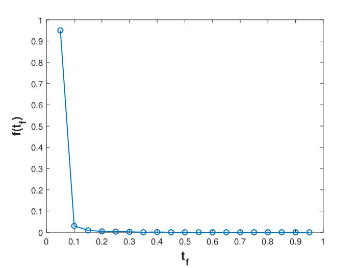
This means that the first-passage time is a deterministic event, occurring at CA​bC_{Ab} with probability 11; see the distribution of first passage time tft_{f} in Fig. 3. Furthermore, for 0<b<1<A0<b<1<A, CA​bC_{Ab} is monotonously increasing of bb but decreasing of AA, being the same as physical intuition.
Refer to caption
Figure 3: PDF of the first passage time of a particle in the box [−1,1][-1,1] starting at −b-b and reaching x=0x=0 for the first time. We simulate it with 10001000 trajectories and the total time T=10T=10. The parameters are b=1/2,A=2b=1/2,\,A=2, and then CA​b=0.0565C_{Ab}=0.0565, which is consistent with the curve that has a peak near 0.05650.0565 in the figure.

III.2 Area under the random walk curve

Now we turn to an application of the Langevin system containing a force field and non-Gaussian β\beta-stable noise. In this case, we take U⁡(x)=xU(x)=x and get the functional Ax=∫0tx⁡(t′)​d​t′A_{x}=\int_{0}^{t}x(t^{\prime})dt^{\prime}, denoting the total area under the curve of trajectory x⁡(t)x(t) [44, 45]. This functional AxA_{x} is also related to the phase accumulated by spins in an NMR experiment [45]. Since the analytical solutions of Gx0​(p,t)G_{x_{0}}(p,t) in (24) cannot be easily obtained due to the Riesz space fractional derivative operator ∇xβ\nabla_{x}^{\beta}, we resort to the forward Feynman-Kac equation (14) by integrating the solution G⁡(x,p,t)G(x,p,t) over xx with initial position x0x_{0} to get the marginal PDF of Gx0​(p,t)G_{x_{0}}(p,t).

In the case of a quadratic potential, where V⁡(x,t)=b​x2/2​(b>0)V(x,t)=bx^{2}/2\,(b>0), (f(x,t)=−∂V(x,t)/∂x=−bxf(x,t)=-\partial V(x,t)/\partial x=-bx) and g⁡(x,t)≡1g(x,t)\equiv 1, U⁡(x)=xU(x)=x, α=1\alpha=1, the forward Feynman-Kac equation (10) takes the form

∂G⁡(k,p,t)∂t+(b​k−p)​∂∂k​G​(k,p,t)=ϕ0​(k)​G​(k,p,t).\frac{\partial G(k,p,t)}{\partial t}+(bk-p)\frac{\partial}{\partial k}G(k,p,t)=\phi_{0}(k)G(k,p,t).

Its general solution is given by the following [46]:

G⁡(k,p,t)=exp⁡[∫0kϕ0​(z)b​z−p​dz+c1]⋅Ψ⁡[1b​ln⁡|b​k−p|−t+c2],\begin{split}G(k,p,t)=&~\exp\left[\int_{0}^{k}\frac{\phi_{0}(z)}{bz-p}dz+c_{1}\right]\\ &~\cdot\Psi\left[\frac{1}{b}\ln|bk-p|-t+c_{2}\right],\end{split} (38)

where c1,c2c_{1},c_{2} are constants and Ψ⁡(x)\Psi(x) is an arbitrary function. Using the initial condition G⁡(k,p,0)=1G(k,p,0)=1 (the particle starts at x0=0x_{0}=0), we get

Ψ[1bln|bk−p|+c2]=exp[−∫0kϕ0​(z)b​z−pdz−c1].\Psi\left[\frac{1}{b}\ln|bk-p|+c_{2}\right]=\exp\left[-\int_{0}^{k}\frac{\phi_{0}(z)}{bz-p}dz-c_{1}\right]. (39)

Then replacing kk by l⁡(k):=b​k−pb​eb​t+pbl(k):=\frac{bk-p}{be^{bt}}+\frac{p}{b} in (39) yields

Ψ[1bln|bk−p|−t+c2]=exp[−∫0l⁡(k)ϕ0​(z)b​z−pdz−c1].\Psi\left[\frac{1}{b}\ln|bk-p|-t+c_{2}\right]=\exp\left[-\int_{0}^{l(k)}\frac{\phi_{0}(z)}{bz-p}dz-c_{1}\right].

Substituting this result into (38), we obtain

G⁡(k,p,t)=exp⁡[∫l⁡(k)kϕ0​(z)b​z−p​𝑑z].G(k,p,t)=\exp\left[\int_{l(k)}^{k}\frac{\phi_{0}(z)}{bz-p}dz\right].

Letting k=0k=0, we get the PDF of functional AxA_{x} in Fourier space (Ax→p)(A_{x}\rightarrow p):

G⁡(p,t):=G⁡(k,p,t)|k=0=exp⁡[∫pb​(1−e−b​t)0ϕ0​(z)b​z−p​𝑑z].G(p,t):=G(k,p,t)|_{k=0}=\exp\left[\int_{\frac{p}{b}(1-e^{-bt})}^{0}\frac{\phi_{0}(z)}{bz-p}dz\right]. (40)

Now we discuss the specific dynamical behaviour of functional AxA_{x} with Lévy β\beta-stable noise (ϕ0​(k)=−|k|β\phi_{0}(k)=-|k|^{\beta}). Considering a variable substitution z=pb​(1−e−b​t)​yz=\frac{p}{b}(1-e^{-bt})y in (40), we obtain

ln⁡G⁡(p,t)=−Cb​(t)​(1−e−b​tb)β+1​|p|β,\ln G(p,t)=-C_{b}(t)\left(\frac{1-e^{-bt}}{b}\right)^{\beta+1}|p|^{\beta}, (41)

where Cb​(t)C_{b}(t) is independent of pp [47]:

Cb​(t)=∫01yβ1−(1−e−b​t)​y​𝑑y=B⁡(β+1,1)⋅F12​(1,β+1,β+2,1−e−b​t).\begin{split}C_{b}(t)&=\int_{0}^{1}\frac{y^{\beta}}{1-(1-e^{-bt})y}dy\\ &=B(\beta+1,1)\cdot{}_{2}F_{1}(1,\beta+1;\beta+2;1-e^{-bt}).\end{split}

It can be seen from (41) that the functional AxA_{x} also obeys Lévy β\beta-stable distribution. Next what we need to pay attention to is the coefficient in front of |p|β|p|^{\beta} in (41).

For long times t→∞t\rightarrow\infty, we find that

Cb​(t)=∫01yβ1−(1−e−b​t)​y​𝑑y≃b​t,C_{b}(t)=\int_{0}^{1}\frac{y^{\beta}}{1-(1-e^{-bt})y}dy\simeq bt,

since this integral scales as b​tbt in both two extreme cases (β=0\beta=0 and β=2\beta=2). Substituting it into (41), we get

G⁡(p,t)≃exp⁡(−b−β​t​|p|β)as​t→∞.G(p,t)\simeq\exp(-b^{-\beta}t|p|^{\beta})~~~~~~\textrm{as}~~~t\rightarrow\infty. (42)

For short times t→0t\rightarrow 0, F12​(1,β+1,β+2,1−e−b​t)∼1{}_{2}F_{1}(1,\beta+1;\beta+2;1-e^{-bt})\sim 1, and thus

G⁡(p,t)≃exp⁡(−tβ+1β+1​|p|β)as​t→0.G(p,t)\simeq\exp\left(-\frac{t^{\beta+1}}{\beta+1}|p|^{\beta}\right)~~~~~~\textrm{as}~~~t\rightarrow 0. (43)

For the special case β=2\beta=2, i.e., Gaussian white noise, by the formula

⟨Ax2⟩=∂2∂p2​G​(p,t)|p=0,\langle A_{x}^{2}\rangle=\left.\frac{\partial^{2}}{\partial p^{2}}G(p,t)\right|_{p=0},

we get

⟨Ax2⟩≃2​b−2​t,as​t→∞,\langle A_{x}^{2}\rangle\simeq 2b^{-2}t,~~~~~~\textrm{as}~~~t\rightarrow\infty, (44)

and

⟨Ax2⟩≃23​t3,as​t→0,\langle A_{x}^{2}\rangle\simeq\frac{2}{3}t^{3},~~~~~~\textrm{as}~~~t\rightarrow 0, (45)

which are verified by numerical simulations. In Fig. 4, the functional AxA_{x} exhibits a crossover between different scaling regimes (from t3t^{3} to tt). When the particle begins its movement from the origin, i.e., x≪1x\ll 1, the effect of force (f=−b​xf=-bx) can be omitted. As time goes on, this effect is getting bigger and bigger, and eventually produces the multi-scale phenomenon. On the contrary, for the case without the force field ff, i.e., b=0b=0, it is equivalent to that b→0b\rightarrow 0 for any tt from (41). Then only the single-scale phenomenon ⟨Ax2⟩≃23​t3\langle A_{x}^{2}\rangle\simeq\frac{2}{3}t^{3} can be observed, which is consistent with [25] by taking α=1\alpha=1 there.

Refer to caption
Figure 4: (Color online) Second moment ⟨Ax2⟩\langle A_{x}^{2}\rangle of the area under the trajectory curve with β=2\beta=2 and b=2b=2, generated with 10001000 trajectories and the total time T=100T=100. The circle-markers denote the simulation results. The dotted line denotes the theoretical result ⟨Ax2⟩≃23​t3\langle A_{x}^{2}\rangle\simeq\frac{2}{3}t^{3} for short time while the solid line represents ⟨Ax2⟩≃2b2​t\langle A_{x}^{2}\rangle\simeq\frac{2}{b^{2}}t for long time. This figure shows a crossover of scaling regimes from t3t^{3} to tt.

As for the general case 0<β<20<\beta<2, the mean squared displacement of AxA_{x} diverges [48]: ⟨Ax2⟩→∞\langle A_{x}^{2}\rangle\rightarrow\infty. But for a particle with non-diverging mass, a finite velocity of propagation exists, making long instantaneous jumps impossible. Their fractional moments can be written as

⟨|Ax|δ⟩∝t~δ/β,\langle|A_{x}|^{\delta}\rangle\propto\tilde{t}^{\delta/\beta}, (46)

where 0<δ<β<20<\delta<\beta<2. From (42) and (43), one can get that in (46) t~\tilde{t} should be tβ+1t^{\beta+1} for short times and tt for long times. So we rescale the fractional moments and get the pseudo second moment [Ax2]∝t~2/β[A_{x}^{2}]\propto\tilde{t}^{2/\beta}. An alternative method is to consider the (Ax−t)(A_{x}-t) scaling relations, or to measure the width of the PDF G⁡(Ax,t)G(A_{x},t) rather than its variance [48]. More precisely, enclose the particle in an imaginary growing box [19] and define

⟨Ax2⟩L:=∫L1​t1/βL2​t1/βAx2​G​(Ax,t)​d​Ax≃t~2/β,\langle A_{x}^{2}\rangle_{L}:=\int_{L_{1}t^{1/\beta}}^{L_{2}t^{1/\beta}}A_{x}^{2}G(A_{x},t)dA_{x}\simeq\tilde{t}^{2/\beta},

where L1L_{1} and L2L_{2} are chosen to adapt the scaling regimes in (42) and (43), i.e., for long time −L1=L2=2​b−β-L_{1}=L_{2}=\sqrt{2b^{-\beta}} while for short time −L1=L2=2/(1+β)-L_{1}=L_{2}=\sqrt{2/(1+\beta)}. This has been implemented numerically and can be seen in Fig. 5. We take β\beta to be 1.41.4 or 0.70.7 and b=2b=2. The markers denote simulation results while the solid lines are the theoretical ones

⟨Ax2⟩≃2​b−β​t2/β,as​t→∞,\langle A_{x}^{2}\rangle\simeq 2b^{-\beta}t^{2/\beta},~~~~~~\textrm{as}~~~t\rightarrow\infty,

and

⟨Ax2⟩≃2β+1​t2​(β+1)/β,as​t→0,\langle A_{x}^{2}\rangle\simeq\frac{2}{\beta+1}t^{2(\beta+1)/\beta},~~~~~~\textrm{as}~~~t\rightarrow 0,

which go back to (44) and (45), respectively, when β=2\beta=2.

Refer to caption
Figure 5: (Color online) Pseudo second moment ⟨Ax2⟩L\langle A_{x}^{2}\rangle_{L} by a cut-off approach, generated with 10001000 trajectories and the total time T=100T=100 with β=1.4, 0.7,\beta=1.4,\,0.7, and b=2b=2. The circle-markers and square-markers denote the simulation results of β=1.4\beta=1.4 and β=0.7\beta=0.7, respectively. The solid lines are the theoretical results with slope 2​(β+1)/β2(\beta+1)/\beta for short time and 2/β2/\beta for long time. It shows that for different Lévy β\beta-stable noise (0<β<20<\beta<2), there is a crossover of scaling regimes from t2​(β+1)/βt^{2(\beta+1)/\beta} to t2/βt^{2/\beta}.

IV Summary and discussion

The Feynman-Kac equations have striking advantages in characterizing the PDFs of various general statistical quantities. Under the CTRW framework, there have been a systematic derivations of the equations. But the CTRW models can not well describe the multiplicative noise and the arbitrary additive noise together with force field, being more conveniently modeled by the Langevin system.

The contributions of the paper are twofold: deriving the forward Feynman-Kac equation from the overdamped Langevin equation driven by an arbitrary Lévy noise together with a time-dependent multiplicative noise term and an arbitrary time-dependent external force field; and deriving the backward Feynman-Kac equation with an arbitrary additive Lévy noise or a multiplicative Gaussian white noise, together with an arbitrary force field. For some special noises and force fields, the obtained equations are consistent with the existing works. Two applications of the derived equations to solve PDFs of the occupation time T+T_{+} and the total area AxA_{x} under the curve of the particle trajectory are carefully provided. In the first application, we take a multiplicative Gaussian white noise and restrict the particle in a box [−L,L][-L,L] with reflecting boundary conditions. Then we find a new phenomenon that for long times the PDF of occupation fraction is a δ\delta-function. In the second application, we take an additive Lévy β\beta-stable noise and find that the AxA_{x} also obeys Lévy stable distribution but experiences a crossover between different scaling regimes.

Using the techniques of subordinator in deriving Feynman-Kac equations presented in [32], we also derive the forward Feynman-Kac equations from the coupled Langevin equation with α\alpha-stable subordinator and arbitrary Lévy noise based on the Langevin framework.

Acknowledgements.
This work was supported by the National Natural Science Foundation of China under grant no. 11671182, and the Fundamental Research Funds for the Central Universities under grants no. lzujbky-2018-ot03 and no. lzujbky-2017-ot10.

Appendix A Forward Feynman-Kac equation with subordinator

Since the forward Feynman-Kac equation in the case of Gaussian white noise ξ⁡(s)\xi(s) has been derived in [32], we can make the best of some techniques of subordinator in that paper and extend its result to arbitrary Lévy noise ξ⁡(s)\xi(s) in the Langevin framework. Some of the calculations about subordinator may be omitted for simplicity; see [32] for the details.

Since y⁡(t)=x⁡(S⁡(t))y(t)=x(S(t)), we can build the Langevin equation of y⁡(t)y(t) from model (11) as:

y˙​(t)=f⁡(y⁡(t),t)​S˙​(t)+g⁡(y⁡(t),t)​ξ​(S⁡(t))​S˙​(t).\dot{y}(t)=f(y(t),t)\dot{S}(t)+g(y(t),t)\xi(S(t))\dot{S}(t).

Being similar to (2), with the Itô interpretation, the increment of y⁡(t)y(t) reads

δ​y​(t)=f⁡(y⁡(t),t)​δ​S​(t)+g⁡(y⁡(t),t)​δ​η​(S⁡(t)),\delta y(t)=f(y(t),t)\delta S(t)+g(y(t),t)\delta\eta(S(t)), (47)

where δ​S​(t)=S⁡(t+τ)−S⁡(t)\delta S(t)=S(t+\tau)-S(t) and δ​η​(S⁡(t))=η⁡(S⁡(t+τ))−η⁡(S⁡(t))\delta\eta(S(t))=\eta(S(t+\tau))-\eta(S(t)). Next, similar to (6), we obtain the increment of G⁡(y,W,t)G(y,W,t) in Fourier space (y→k,W→p)(y\rightarrow k,W\rightarrow p):

δ​G​(k,p,t)=⟨e−i​k​y​(t)−i​p​W​(t)​(e−i​k​g​(y⁡(t),t)​δ​η​(S⁡(t))−1)⟩−i​k​⟨e−i​k​y​(t)−i​p​W​(t)​f​(y⁡(t),t)​δ​S​(t)⟩−i​p​τ​⟨e−i​k​y​(t)−i​p​W​(t)​U​(y⁡(t))⟩,\begin{split}\delta G(k,p,t)=&~\langle e^{-iky(t)-ipW(t)}(e^{-ikg(y(t),t)\delta\eta(S(t))}-1)\rangle\\ &-ik\langle e^{-iky(t)-ipW(t)}f(y(t),t)\delta S(t)\rangle\\ &-ip\tau\langle e^{-iky(t)-ipW(t)}U(y(t))\rangle,\end{split} (48)

where the first term on the right hand side can be reduced to

⟨e−i​k​y​(t)−i​p​W​(t)​ϕ0​(k​g​(y⁡(t),t))​δ​S​(t)⟩\langle e^{-iky(t)-ipW(t)}\phi_{0}(kg(y(t),t))\,\delta S(t)\rangle

as usual by the characteristic function of δ​η​(t)\delta\eta(t) in (3). So dividing (48) by τ\tau and taking the limit τ→0\tau\rightarrow 0, we obtain

∂∂t​G​(k,p,t)=⟨e−i​k​y​(t)−i​p​W​(t)​ϕ0​(k​g​(y⁡(t),t))​S˙​(t)⟩−i​k​⟨e−i​k​y​(t)−i​p​W​(t)​f​(y⁡(t),t)​S˙​(t)⟩−i​p​⟨e−i​k​y​(t)−i​p​W​(t)​U​(y⁡(t))⟩=:Q1+Q2+Q3.\begin{split}\frac{\partial}{\partial t}G(k,p,t)=&~\langle e^{-iky(t)-ipW(t)}\phi_{0}(kg(y(t),t))\dot{S}(t)\rangle\\ &-ik\langle e^{-iky(t)-ipW(t)}f(y(t),t)\dot{S}(t)\rangle\\ &-ip\langle e^{-iky(t)-ipW(t)}U(y(t))\rangle\\ =&:~Q_{1}+Q_{2}+Q_{3}.\end{split} (49)

It is obvious that the inverse Fourier transform (k→yk\rightarrow y) of Q3Q_{3} is −i​p​U​(y)​G​(y,p,t)-ipU(y)G(y,p,t). But for Q1Q_{1} and Q2Q_{2}, they look a little bit difficult due to the new term S˙​(t)\dot{S}(t) compared with (6). Note that the angle bracket in Q1Q_{1} denotes the average of two kinds of independent stochastic processes with the joint PDF G⁡(y⁡(t),W⁡(t),t)G(y(t),W(t),t) and Lévy α\alpha-stable noise θ⁡(t)\theta(t) on which S⁡(t)S(t) depends. To deal with the term Q1Q_{1}, we first add a technical delta function δ⁡(y−y⁡(t))\delta(y-y(t)) in it and get

Q1=∫−∞∞e−i​k​y​ϕ0​(k​g​(y,t))​⟨e−i​p​W​(t)​δ​(y−y⁡(t))​S˙​(t)⟩​𝑑y.Q_{1}=\int_{-\infty}^{\infty}e^{-iky}\phi_{0}(kg(y,t))\langle e^{-ipW(t)}\delta(y-y(t))\dot{S}(t)\rangle dy.

Then applying the technique in [32] of rewriting the functional W⁡(t)W(t) as a subordinated process:

W⁡(t)=V⁡(S⁡(t)),V⁡(s)=∫0sU⁡(x⁡(s′))​θ​(s′)​d​s′.W(t)=V(S(t)),\qquad V(s)=\int_{0}^{s}U(x(s^{\prime}))\theta(s^{\prime})ds^{\prime}.

Substituting y⁡(t)=x⁡(S⁡(t))y(t)=x(S(t)) and W⁡(t)=V⁡(S⁡(t))W(t)=V(S(t)) into Q1Q_{1} gives the middle term of Q1Q_{1} as

⟨e−i​p​V​(S⁡(t))​δ​(y−x⁡(S⁡(t)))​S˙​(t)⟩=∫0∞⟨e−i​p​V​(s)​δ​(y−x⁡(s))​δ​(t−T⁡(s))⟩​ds.\begin{split}&\langle e^{-ipV(S(t))}\delta(y-x(S(t)))\dot{S}(t)\rangle\\ &=\int_{0}^{\infty}\langle e^{-ipV(s)}\delta(y-x(s))\delta(t-T(s))\rangle ds.\end{split} (50)

Taking Laplace transform (t→ut\rightarrow u) of (50), we obtain

Q1​(u)=∫−∞∞e−i​k​y​ϕ0​(k​g​(y,t))⋅∫0∞⟨e−i​p​V​(s)−u​T​(s)​δ​(y−x⁡(s))⟩​ds​dy.\begin{split}Q_{1}(u)=&~\int_{-\infty}^{\infty}e^{-iky}\phi_{0}(kg(y,t))\\ &\cdot\int_{0}^{\infty}\langle e^{-ipV(s)-uT(s)}\delta(y-x(s))\rangle dsdy.\end{split} (51)

On the other hand, G⁡(y,p,t)G(y,p,t) can be rewritten as:

G⁡(y,p,t)=⟨e−i​p​V​(S⁡(t))​δ​(y−x⁡(S⁡(t)))⟩=∫0∞⟨e−i​p​V​(s)​δ​(s−S⁡(t))​δ​(y−x⁡(s))⟩​ds.\begin{split}G(y,p,t)&=\langle e^{-ipV(S(t))}\delta(y-x(S(t)))\rangle\\ &=\int_{0}^{\infty}\langle e^{-ipV(s)}\delta(s-S(t))\delta(y-x(s))\rangle ds.\end{split}

So its Laplace transform (t→ut\rightarrow u) is

G⁡(y,p,u)=∫0∞⟨e−i​p​V​(s)−u​T​(s)​θ​(s)​δ​(y−x⁡(s))⟩​𝑑s.G(y,p,u)=\int_{0}^{\infty}\langle e^{-ipV(s)-uT(s)}\theta(s)\delta(y-x(s))\rangle ds. (52)

The characteristic function of the Lévy process T⁡(s)T(s) in (11) is

⟨e−u​T​(s)⟩=e−s​uα,\langle e^{-uT(s)}\rangle=e^{-su^{\alpha}},

which yields an important equality in [32] from (52):

G⁡(y,p,u)=[u+i​p​U​(y)]α−1⋅∫0∞⟨e−i​p​V​(s)−u​T​(s)​δ​(y−x⁡(s))⟩​ds.\begin{split}G(y,p,u)=&[u+ipU(y)]^{\alpha-1}\\ &\cdot\int_{0}^{\infty}\langle e^{-ipV(s)-uT(s)}\delta(y-x(s))\rangle ds.\end{split} (53)

Comparing (51) with (53), we find that

Q1​(u)=∫−∞∞e−i​k​y​ϕ0​(k​g​(y,t))​[u+i​p​U​(y)]1−α​G​(y,p,u)​𝑑y.Q_{1}(u)=\int_{-\infty}^{\infty}e^{-iky}\phi_{0}(kg(y,t))[u+ipU(y)]^{1-\alpha}G(y,p,u)dy.

Taking the inverse Laplace transform (u→tu\rightarrow t), we obtain

Q1=∫−∞∞e−i​k​y​ϕ0​(k​g​(y,t))​𝒟t1−α​G​(y,p,t)​𝑑y.Q_{1}=\int_{-\infty}^{\infty}e^{-iky}\phi_{0}(kg(y,t))\mathcal{D}_{t}^{1-\alpha}G(y,p,t)dy. (54)

As for Q2Q_{2}, it can be obtained by the procedure similar to Q1Q_{1}, i.e.,

Q2=−ik∫−∞∞e−i​k​yf(y,t)𝒟t1−αG(y,p,t)dy.Q_{2}=-ik\int_{-\infty}^{\infty}e^{-iky}f(y,t)\mathcal{D}_{t}^{1-\alpha}G(y,p,t)dy. (55)

Finally, substituting (54) and (55) into (49), we obtain the forward Feynman-Kac equation in Fourier space:

∂G⁡(k,p,t)∂t=ℱy​{ϕ0​(k​g​(y,t))​𝒟t1−α​G​(y,p,t)}−ℱy​{∂∂y​f​(y,t)​𝒟t1−α​G​(y,p,t)+i​p​U​(y)​G​(y,p,t)}.\begin{split}&\frac{\partial G(k,p,t)}{\partial t}=\mathcal{F}_{y}\{\phi_{0}(kg(y,t))\mathcal{D}_{t}^{1-\alpha}G(y,p,t)\}\\ &~~-\mathcal{F}_{y}\left\{\frac{\partial}{\partial y}f(y,t)\mathcal{D}_{t}^{1-\alpha}G(y,p,t)+ipU(y)G(y,p,t)\right\}.\end{split}

Appendix B Backward Feynman-Kac equation with multiplicative noise

If g⁡(x)g(x) is not a constant in (15), then the Fourier transform of ⟨Tη⟩\langle T_{\eta}\rangle becomes

ℱy​{⟨Tη⟩}=⟨∫−∞∞e−i​k0​x​(τ)​Tη​ei​k0​(f⁡(x0)​τ+g⁡(x0)​η​(τ))​d​x0⟩.\mathcal{F}_{y}\{\langle T_{\eta}\rangle\}=\left\langle\int_{-\infty}^{\infty}e^{-ik_{0}x(\tau)}T_{\eta}e^{ik_{0}(f(x_{0})\tau+g(x_{0})\eta(\tau))}dx_{0}\right\rangle.

We turn d​x0dx_{0} into d​x​(τ)dx(\tau) and get

ℱx0​{⟨Tη⟩}=⟨∫−∞∞e−i​k0​x​(τ)​Tη​ei​k0​(f⁡(x0)​τ+g⁡(x0)​η​(τ))​𝑑x​(τ)⟩−⟨∫−∞∞e−i​k0​x​(τ)​Tη​ei​k0​(f⁡(x0)​τ+g⁡(x0)​η​(τ))​d​f​(x0)d​x0​τ​d​x0⟩−⟨∫−∞∞e−i​k0​x​(τ)​Tη​ei​k0​(f⁡(x0)​τ+g⁡(x0)​η​(τ))​d​g​(x0)d​x0​η​(τ)​d​x0⟩.\begin{split}\mathcal{F}_{x_{0}}\{\langle T_{\eta}\rangle\}=&~\Big\langle\int_{-\infty}^{\infty}e^{-ik_{0}x(\tau)}T_{\eta}e^{ik_{0}(f(x_{0})\tau+g(x_{0})\eta(\tau))}dx(\tau)\Big\rangle-\Big\langle\int_{-\infty}^{\infty}e^{-ik_{0}x(\tau)}T_{\eta}e^{ik_{0}(f(x_{0})\tau+g(x_{0})\eta(\tau))}\frac{df(x_{0})}{dx_{0}}\tau dx_{0}\Big\rangle\\ &-\Big\langle\int_{-\infty}^{\infty}e^{-ik_{0}x(\tau)}T_{\eta}e^{ik_{0}(f(x_{0})\tau+g(x_{0})\eta(\tau))}\frac{dg(x_{0})}{dx_{0}}\eta(\tau)dx_{0}\Big\rangle.\end{split} (56)

Letting τ→0\tau\rightarrow 0, the second term of ℱx0​{⟨Tη⟩}\mathcal{F}_{x_{0}}\{\langle T_{\eta}\rangle\} is the same as (21), i.e.,

−τ​ℱx0​{∂f⁡(x0)∂x0​Gx0​(p,t)}.-\tau\mathcal{F}_{x_{0}}\Big\{\frac{\partial f(x_{0})}{\partial x_{0}}G_{x_{0}}(p,t)\Big\}. (57)

Though η⁡(τ)→0\eta(\tau)\rightarrow 0 as τ→0\tau\rightarrow 0, how fast it tends to 00 is not specific, which arises the challenge of dealing with the first and third terms (56). To make this point clear, we should define

Mn​(k,τ)=⟨e−i​k​η​(τ)​ηn​(τ)⟩.M_{n}(k,\tau)=\langle e^{-ik\eta(\tau)}\eta^{n}(\tau)\rangle.

When n=0n=0, M0M_{0} is the characteristic function of η⁡(τ)\eta(\tau), given in (3). When n≥1n\geq 1, Mn→0M_{n}\rightarrow 0 as τ→0\tau\rightarrow 0. For the case of Gaussian white noise: M0=e−τ​k2M_{0}=e^{-\tau k^{2}}, by some calculations, we have, as τ→0\tau\rightarrow 0,

M1∼−2ikτ,M2∼2τ,Mn∼τ2∼0∀n≥3;\begin{split}&M_{1}\sim-2ik\tau,\qquad M_{2}\sim 2\tau,\\ &M_{n}\sim\tau^{2}\sim 0\qquad\forall~n\geq 3;\end{split} (58)

since Mn​(n≥3)M_{n}\,(n\geq 3) are all higher order terms of τ\tau, it can be omitted. But for Lévy β\beta-stable noise, M0=e−τ​|k|βM_{0}=e^{-\tau|k|^{\beta}} and all Mn​(n≥1)M_{n}\,(n\geq 1) contain the first order term of τ\tau. Here we focus on the case that η⁡(τ)\eta(\tau) is Gaussian white noise, and use the property (58) to deal with the first and third terms in (56).

Denoting the first term as T1T_{1} for convenient and using ei​k0​f​(x0)​τ≃1+i​k0​f​(x0)​τe^{ik_{0}f(x_{0})\tau}\simeq 1+ik_{0}f(x_{0})\tau as before, we get

T1=⟨∫−∞∞e−i​k0​x​(τ)​Tη​ei​k0​g​(x0)​η​(τ)​𝑑x​(τ)⟩+i​k0​τ​⟨∫−∞∞e−i​k0​x​(τ)​Tη​f​(x⁡(τ))​𝑑x​(τ)⟩,T_{1}=\Big\langle\int_{-\infty}^{\infty}e^{-ik_{0}x(\tau)}T_{\eta}e^{ik_{0}g(x_{0})\eta(\tau)}dx(\tau)\Big\rangle+ik_{0}\tau\Big\langle\int_{-\infty}^{\infty}e^{-ik_{0}x(\tau)}T_{\eta}f(x(\tau))dx(\tau)\Big\rangle, (59)

where the latter term equals to

τ​ℱx0​{∂∂x0​f​(x0)​Gx0​(p,t)}.\tau\mathcal{F}_{x_{0}}\Big\{\frac{\partial}{\partial x_{0}}f(x_{0})G_{x_{0}}(p,t)\Big\}.

Turn g⁡(x0)g(x_{0}) into g⁡(x⁡(τ))g(x(\tau)) in (59) by Taylor expansion g⁡(x0)=g⁡(x⁡(τ))+Rgg(x_{0})=g(x(\tau))+R_{g}, where

Rg=−(f⁡(x0)​τ+g⁡(x0)​η​(τ))​g′​(x⁡(τ))+12​(f⁡(x0)​τ+g⁡(x0)​η​(τ))2​g′′​(x⁡(τ))+⋯,\begin{split}R_{g}=-(f(x_{0})\tau+g(x_{0})\eta(\tau))g^{\prime}(x(\tau))+\frac{1}{2}(f(x_{0})\tau+g(x_{0})\eta(\tau))^{2}g^{\prime\prime}(x(\tau))+\cdots,\end{split}

and here for convenient, we use the notation ′ to denote the first order derivative. Then the former term of (59), denoted as T11T_{11}, becomes

T11=⟨∫−∞∞e−i​k0​x​(τ)​Tη​ei​k0​g​(x⁡(τ))​η​(τ)​ei​k0​Rg​η​(τ)​𝑑x​(τ)⟩,T_{11}=\Big\langle\int_{-\infty}^{\infty}e^{-ik_{0}x(\tau)}T_{\eta}e^{ik_{0}g(x(\tau))\eta(\tau)}e^{ik_{0}R_{g}\eta(\tau)}dx(\tau)\Big\rangle, (60)

where ei​k0​Rg​η​(τ)=1+i​k0​Rg​η​(τ)+⋯e^{ik_{0}R_{g}\eta(\tau)}=1+ik_{0}R_{g}\eta(\tau)+\cdots. Considering Mn∼0​(n≥3)M_{n}\sim 0\,(n\geq 3) in (58), the second term of RgR_{g} and all the latter terms can be omitted since these terms contribute to η2​(τ)\eta^{2}(\tau) and then yields Mn​(n≥3)M_{n}\,(n\geq 3) when substituted into (60). Therefore, we have

T11=⟨∫−∞∞e−i​k0​x​(τ)​Tη​ei​k0​g​(x⁡(τ))​η​(τ)​e−i​k0​g​(x0)​g′​(x⁡(τ))​η2​(τ)​𝑑x​(τ)⟩=⟨∫−∞∞e−i​k0​x​(τ)​Tη​ei​k0​g​(x⁡(τ))​η​(τ)​𝑑x​(τ)⟩−i​k0​⟨∫−∞∞e−i​k0​x​(τ)​Tη​ei​k0​g​(x⁡(τ))​η​(τ)​g​(x0)​g′​(x⁡(τ))​η2​(τ)​𝑑x​(τ)⟩=ℱx0​{⟨ei​k0​g​(x0)​η​(τ)⟩​Gx0​(p,t)}−i​k0​ℱx0​{⟨ei​k0​g​(x0)​η​(τ)​η2​(τ)⟩​g​(x0)​g′​(x0)​Gx0​(p,t)},\begin{split}T_{11}&=\Big\langle\int_{-\infty}^{\infty}e^{-ik_{0}x(\tau)}T_{\eta}e^{ik_{0}g(x(\tau))\eta(\tau)}e^{-ik_{0}g(x_{0})g^{\prime}(x(\tau))\eta^{2}(\tau)}dx(\tau)\Big\rangle\\ &=\Big\langle\int_{-\infty}^{\infty}e^{-ik_{0}x(\tau)}T_{\eta}e^{ik_{0}g(x(\tau))\eta(\tau)}dx(\tau)\Big\rangle-ik_{0}\Big\langle\int_{-\infty}^{\infty}e^{-ik_{0}x(\tau)}T_{\eta}e^{ik_{0}g(x(\tau))\eta(\tau)}g(x_{0})g^{\prime}(x(\tau))\eta^{2}(\tau)dx(\tau)\Big\rangle\\ &=\mathcal{F}_{x_{0}}\{\langle e^{ik_{0}g(x_{0})\eta(\tau)}\rangle G_{x_{0}}(p,t)\}-ik_{0}\mathcal{F}_{x_{0}}\{\langle e^{ik_{0}g(x_{0})\eta(\tau)}\eta^{2}(\tau)\rangle g(x_{0})g^{\prime}(x_{0})G_{x_{0}}(p,t)\},\end{split}

where we replace g⁡(x0)g(x_{0}) by g⁡(x⁡(τ))g(x(\tau)) in the latter term and omit the high order term M3M_{3}. Substituting M2M_{2} in (58) and T11T_{11} into (59) gives

T1=ℱx0​{⟨ei​k0​g​(x0)​η​(τ)⟩​Gx0​(p,t)}−2​i​k0​τ​ℱx0​{g⁡(x0)​g′​(x0)​Gx0​(p,t)}+τ​ℱx0​{∂∂x0​f​(x0)​Gx0​(p,t)}.T_{1}=\mathcal{F}_{x_{0}}\{\langle e^{ik_{0}g(x_{0})\eta(\tau)}\rangle G_{x_{0}}(p,t)\}-2ik_{0}\tau\mathcal{F}_{x_{0}}\{g(x_{0})g^{\prime}(x_{0})G_{x_{0}}(p,t)\}+\tau\mathcal{F}_{x_{0}}\Big\{\frac{\partial}{\partial x_{0}}f(x_{0})G_{x_{0}}(p,t)\Big\}. (61)

Similarly, still using the property Mn∼0,n≥3M_{n}\sim 0,\,n\geq 3, we get the third term in (56),

T3=−2​τ​ℱx0​{g⁡(x0)​g′​(x0)​∂Gx0​(p,t)∂x0}.T_{3}=-2\tau\mathcal{F}_{x_{0}}\Big\{g(x_{0})g^{\prime}(x_{0})\frac{\partial G_{x_{0}}(p,t)}{\partial x_{0}}\Big\}. (62)

Combining (61), (62) and (57), we finally get

ℱx0​{⟨Tη⟩}=ℱx0​{⟨ei​k0​g​(x0)​η​(τ)⟩​Gx0​(p,t)}−2​τ​ℱx0​{∂∂x0​g​(x0)​g′​(x0)​Gx0​(p,t)}+τ​ℱx0​{f⁡(x0)​∂Gx0​(p,t)∂x0}−2​τ​ℱx0​{g⁡(x0)​g′​(x0)​∂Gx0​(p,t)∂x0}.\begin{split}\mathcal{F}_{x_{0}}\{\langle T_{\eta}\rangle\}=&~\mathcal{F}_{x_{0}}\{\langle e^{ik_{0}g(x_{0})\eta(\tau)}\rangle G_{x_{0}}(p,t)\}-2\tau\mathcal{F}_{x_{0}}\Big\{\frac{\partial}{\partial x_{0}}g(x_{0})g^{\prime}(x_{0})G_{x_{0}}(p,t)\Big\}\\ &+\tau\mathcal{F}_{x_{0}}\Big\{f(x_{0})\frac{\partial G_{x_{0}}(p,t)}{\partial x_{0}}\Big\}-2\tau\mathcal{F}_{x_{0}}\Big\{g(x_{0})g^{\prime}(x_{0})\frac{\partial G_{x_{0}}(p,t)}{\partial x_{0}}\Big\}.\end{split} (63)

Using the characteristic function of Lévy noise (3) leads to

⟨ei​k0​g​(x0)​η​(τ)⟩−1≃τ​ϕ0​(−k0​g​(x0))=−τ​k02​g2​(x0)as​τ→0.\langle e^{ik_{0}g(x_{0})\eta(\tau)}\rangle-1\simeq\tau\phi_{0}(-k_{0}g(x_{0}))=-\tau k_{0}^{2}g^{2}(x_{0})\qquad\textrm{as}~\tau\rightarrow 0. (64)

Combining (63) and (64), by some calculations, we obtain

ℱx0​{⟨Tη⟩}−ℱx0​{Gx0​(p,t)}=τ​ℱx0​{g2​(x0)​∂2Gx0​(p,t)∂x02}+τ​ℱx0​{f⁡(x0)​∂Gx0​(p,t)∂x0}.\mathcal{F}_{x_{0}}\{\langle T_{\eta}\rangle\}-\mathcal{F}_{x_{0}}\{G_{x_{0}}(p,t)\}=\tau\mathcal{F}_{x_{0}}\Big\{g^{2}(x_{0})\frac{\partial^{2}G_{x_{0}}(p,t)}{\partial x_{0}^{2}}\Big\}+\tau\mathcal{F}_{x_{0}}\Big\{f(x_{0})\frac{\partial G_{x_{0}}(p,t)}{\partial x_{0}}\Big\}.

Substituting this formula into (19), dividing (19) by τ\tau, taking the limit τ→0\tau\rightarrow 0 and making the inverse Fourier transform (k0→x0k_{0}\rightarrow x_{0}), we obtain the backward Feynman-Kac equation:

∂Gx0​(p,t)∂t=g2​(x0)​∂2Gx0​(p,t)∂x02+f⁡(x0)​∂Gx0​(p,t)∂x0−i​p​U​(x0)​Gx0​(p,t).\frac{\partial G_{x_{0}}(p,t)}{\partial t}=g^{2}(x_{0})\frac{\partial^{2}G_{x_{0}}(p,t)}{\partial x_{0}^{2}}+f(x_{0})\frac{\partial G_{x_{0}}(p,t)}{\partial x_{0}}-ipU(x_{0})G_{x_{0}}(p,t). (65)

References

  • [1] M. Kac, Trans. Amer. Math. Soc. 65, 1 (1949).
  • [2] H. Geman and M. Yor, Math. Finance 3, 349 (1993).
  • [3] A. Comtet, J. Desbois, and C. Texier, J. Phys. A 38, R341 (2005).
  • [4] S. N. Majumdar, Current Sci. 89, 2076 (2005).
  • [5] S. N. Majumdar and A. J. Bray, Phys. Rev. E 65, 051112 (2002).
  • [6] P. Langevin, C. R. Acad. Sci. 146, 530 (1908).
  • [7] W. T. Coffey, Y. P. Kalmykov, and J. T. Waldron, The Langevin Equation (World Scientific, Singapore, 2004).
  • [8] D. Applebaum, Lévy Processes and Stochastic Calculus (Cambridge University Press, Cambridge, 2009).
  • [9] N. G. V. Kampen, Stochastic Processes in Physics and Chemistry (North-Holland, Amsterdam, 1992).
  • [10] W. Horsthemke and R. Lefever, Noise-Induced Transitions (Springer-Verlag, Berlin, 1984).
  • [11] P. Hänggi and H. Thomas, Phys. Rep. 88, 207 (1982).
  • [12] H. Risken, The Fokker-Planck Equation (Springer-Verlag, Berlin, 1989).
  • [13] S. I. Denisov, W. Horsthemke, and P. Hänggi, Phys. Rev. E 77, 061112 (2008).
  • [14] S. I. Denisov, W. Horsthemke, and P. Hänggi, Eur. Phys. J. B 68, 567 (2009).
  • [15] H. C. Fogedby, Phys. Rev. E 50, 1657 (1994).
  • [16] H. C. Fogedby, Phys. Rev. E 58, 1690 (1998).
  • [17] K. M. Kolwankar and A. D. Gangal, Phys. Rev. Lett. 80, 214 (1998).
  • [18] R. Metzler, E. Barkai, and J. Klafter, Phys. Rev. Lett. 82, 3563 (1999).
  • [19] S. Jespersen, R. Metzler, and H. C. Fogedby, Phys. Rev. E 59, 2736 (1999).
  • [20] A. V. Chechkin, V. Y. Gonchar, J. Klafter, and R. Metzler, Adv. Chem. Phys. 133, 439 (2006).
  • [21] S. A. Adelman, J. Chem. Phys. 64, 124 (1976).
  • [22] M. Magdziarz and A. Weron, Phys. Rev. E 75, 016708 (2007).
  • [23] L. Turgeman, S. Carmi, and E. Barkai, Phys. Rev. Lett. 103, 190201 (2009).
  • [24] S. Carmi and E. Barkai, Phys. Rev. E 84, 061104 (2011).
  • [25] S. Carmi, L. Turgeman, and E. Barkai, J. Stat. Phys. 141, 1071 (2010).
  • [26] X. C. Wu, W. H. Deng, and E. Barkai, Phys. Rev. E 93, 032151 (2016).
  • [27] R. Hou and W. H. Deng, J. Phys. A 51, 155001 (2018).
  • [28] W. L. Wang and W. H. Deng, J. Phys. A 51, 015001 (2018).
  • [29] P. B. Xu and W. H. Deng, Math. Model. Nat. Phenom 13, 10 (2018).
  • [30] D. Selmeczi, L. Li, L. I. I. Pedersen, S. F. Nrrelykke, P. H. Hagedorn, S. Mosler, N. B. Larsen, E. C. Cox, and H. Flyvbjerg, Eur. Phys. J. Special Topics 157, 1 (2008).
  • [31] A. Cairoli and A. Baule, Phys. Rev. Lett. 115, 110601 (2015).
  • [32] A. Cairoli and A. Baule, J. Phys. A 50, 164002 (2017).
  • [33] K. Ito, Nagoya Math. J. 1, 35 (1950).
  • [34] A. Piryatinska, A. I. Saichev, and W. A. Woyczynski, Physica A 349, 375 (2005).
  • [35] M. Magdziarz, A. Weron, and J. Klafter, Physica A 367, 1 (2006).
  • [36] M. Magdziarz, A. Weron, and J. Klafter, Phys. Rev. Lett. 101, 210601 (2008).
  • [37] E. Heinsalu, M. Patriarca, I. Goychuk, and P. Hänggi, Phys. Rev. Lett. 99, 120602 (2007).
  • [38] R. Friedrich, F. Jenko, A. Baule, and S. Eule, Phys. Rev. Lett. 96, 230601 (2006).
  • [39] I. M. Sokolov and R. Metzler, Phys. Rev. E 67, 010101(R) (2003).
  • [40] J. Klafter and I. M. Sokolov, First Steps in Random Walks From Tools to Applications (Oxford University Press, New York, 2011).
  • [41] C. Godrèche and J. M. Luck, J. Stat. Phys. 104, 489 (2001).
  • [42] S. Redner, A Guide to First-Passage Processes (Cambridge University Press, Cambridge, 2001).
  • [43] M. Kac, On Some Connections between Probability Theory and Differential and Integral Equations (University of California Press, Berkeley, 1951) p. 189.
  • [44] A. Baule and R. Friedrich, Phys. Lett. A 350, 167 (2006).
  • [45] D. S. Grebenkov, Rev. Mod. Phys. 79, 1077 (2007).
  • [46] A. D. Polyanin, V. F. Zaitsev, and A. Moussiaux, Handbook of First-order Partial Differential Equations (Taylor & Francis, London, 2002).
  • [47] I. S. Gradshteyn, I. M. Ryzhik, Y. V. Geraniums, and M. Y. Tseytlin, Table of Integrals, Series, and Products (Academic Press, USA, 1980).
  • [48] R. Metzler and J. Klafter, Phys. Rep. 339, 1 (2000).