Sparse Over-complete Patch Matching
Abstract
Image patch matching, which is the process of identifying corresponding patches across images, has been used as a subroutine for many computer vision and image processing tasks. State -of-the-art patch matching techniques take image patches as input to a convolutional neural network to extract the patch features and evaluate their similarity. Our aim in this paper is to improve on the state of the art patch matching techniques by observing the fact that a sparse-overcomplete representation of an image posses statistical properties of natural visual scenes which can be exploited for patch matching. We propose a new paradigm which encodes image patch details by encoding the patch and subsequently using this sparse representation as input to a neural network to compare the patches. As sparse coding is based on a generative model of natural image patches, it can represent the patch in terms of the fundamental visual components from which it has been composed of, leading to similar sparse codes for patches which are built from similar components. Once the sparse coded features are extracted, we employ a fully-connected neural network, which captures the non-linear relationships between features, for comparison. We have evaluated our approach using the Liberty and Notredame subsets of the popular UBC patch dataset and set a new benchmark outperforming all state-of-the-art patch matching techniques for these datasets. 11 1 This paper is under consideration at Pattern Recognition Letters.
1 Introduction
Image patch matching is a fundamental process used in many image processing applications such as image classification [1], object recognition [41] image stitching [2], and correspondence estimation required for structure from motion [3]. Depending on the application, a patch matching technique may have to deal with different challenges such as intra class variations, different lighting conditions, shadings and occlusions [33]. Patch matching techniques have evolved through decades while trying to tackle these challenges [11, 24, 25].
In the process of patch matching, two key components can be identified: the patch descriptor and the matching function. The patch descriptor is extracted to represent the features of the image patch which are then subjected to the matching function to estimate their similarity. The patch matching techniques have evolved from early stages across both of these components. In the early stages the pixel values were used as the patch features and the distance among pixel values were used to measure the similarity. These types of early stage approaches have been heavily sensitive to slight transformations of the patches [34]. The state-of-the-art patch matching techniques are based on deep learning where the patch descriptor identification and similarity estimation is performed using deep neural networks [4, 5]. These techniques aim to tackle the challenging nature of patch matching including viewpoint change, illuminations variations and different shadings. However the state-of-the-art patch matching techniques predominately focus on visual elements that are present in the current image and they do not effectively consider the composition of underlying object shapes and structures that have contributed to the current image.
Sparse coding is an important concept that is used for the sensory coding in the human brain [6]. In human visual cortex, for each information captured by human eye a neural code is formed by activating a selected set of neurons from a large neural population. Sparse coding has revealed how the human brain can process a new image through the relations it can determine with images it has already come across so far. In this paper, we draw inspiration from this to propose a mechanism where sparse coding is utilised to produce a patch descriptor. In contrast to the state-of-the-art patch matching techniques which use visual deep features of the patch image [4, 5], we consider the statistical representation of the patch image in deducing the descriptor. The study carried out by Gregory Shakhnarovich [34] has concluded that in overcomplete sparse coding a small variation in an image can cause a significant change in the resulting coefficients. Therefore a hand engineered similarity measure may be inadequate for comparing the resultant sparse codes. To accommodate for these nonlinear relationships we use a neural network based mechanism to determine the patch similarity as a neural network is capable of dealing with the heavy variations in the input [35].
2 Related work
The previous work related to image patch matching can be categorized under three categories: approaches using image intensities, approaches using hand engineered features and approaches using deep learned features. Traditional patch matching techniques start with using pixel based distance to identify patch correspondence, where distance was used to compare pixel values of two patch images. The next stage of this category image patch matching has used normalized correlation between patches to identify their correspondence [7, 8]. Calculating image descriptors such as Scale-invariant feature transform (SIFT) [9] and DAISY [10] and estimating the descriptor distance is the main concept behind the hand engineered feature based methods .


In the most recent literature, there are two main approaches which have been motivated by the recent advances in neural networks and deep learning [4, 5]. The aim of these deep learning based patch matching techniques are to generate more robust descriptors which can overcome the drawbacks of hand crafted features such that the descriptors and the matching algorithms are not vulnerable to challenging factors in the patches such as illumination changes , occlusions and shadings.
In the approach suggested by Zagoruyko and Komodakis [5] they have evaluated three main neural network architectures for the patch matching. The architectures they have suggested are 1) Siamese, 2) Pseudo-siamese and 3) 2-channel. The siamese and pseudo-siamese architectures contain two branches and as the input each branch takes one of the two patches to be compared. The output of these two branches are analogous to the feature descriptors in the traditional approaches and the branches are merged at the top to make the comparison. In contrast to the siamese architecture where the weights of the two branches are shared in the pseudo siamese architecture the weights are uncoupled. In 2-channel architecture two patches are considered as a 2 channel image where there is no explicit separation on feature descriptor generation and matching. The evaluations on these architectures have been carried out on UBC dataset [11]. Their evaluations conclude that when the convolution layer was divided into small kernels of size , 2 channel architecture performs the best.
Matchnet [4] is a convolution neural network (CNN) based approach where the architecture consists of two sub components as feature network - to extract the features of the patches and metric network - to model the similarity between the patches. To train the networks they have used cross entropy error. Their evaluations are also based on the standard UBC dataset [11].
Coefficients of an encoding mechanism for a set of images such that the accuracy of reconstruction and the sparseness of coefficient are maximized, can possess statistical properties of natural visual scenes [12, 13]. Sparse coded coefficients have successfully been used in computer vision applications as well as in signal processing applications in general. While some applications of this concept are image classification [22], image reconstruction [23] and audio analysis [27, 28], this concept has not been adopted for patchmatching processes. In the previous approaches of image patch matching visual features have majorly been used. In our approach we use coefficient resulted from over-complete sparse coding of patches (Figure 1, Figure 2) as the feature representation and to estimate the patch similarity we use a neural network while tolerating non linear dependencies in input images.
3 The proposed patch matching framework
The overall flow of our patch matching framework is depicted in Figure 3. First we learn a set of basis (dictionary) based on a randomly selected sample of training data. This dictionary is used to encode the training data as well as the test data. Once the training data has been encoded we use that data to train a neural network in a supervised manner. Then at the testing phase we encode the test data and feed them to the trained model to examine the patch similarity. Section 3.1 elaborates the encoding technique that we used including dictionary learning phase (Section 3.1) and coefficient learning phase (Section 3.1). The details on the neural network architecture that we used for patch matching is elaborated in Section 3.2.

3.1 Patch descriptor
As discussed in the related work section, our approach use over complete sparse representation of image patch as the patch descriptor. In the sparse coding, the dictionary is also denoted as the basis vector and the representation of the image patch with respect to the basis is denoted as the coefficient vector. The term sparse enforces the number of non zero elements in the coefficient vector to be minimized while offering a good discriminative power [30, 31]. The problem of learning the basis vector and the coefficients can be formed as Equation 1 :
| (1) |
where is the data matrix, is the basis vector such that and is the coefficient vector such that . When it is known as undercomplete , complete and overcomplete.
To ensure the minimized reconstruction error, the Equation 2
| (2) |
has to be solved and to ensure the overcompleteness should be greater than . In this work we employ ‘overcomplete’ representation as it has been identified overcomplete representation is better able of capturing patterns that are present in the input image while ensuring a better robustness at the presence for factors such as image degradations, scale changes, translations and rotations [12].
To solve the sparse coding problem we used the method similar to the method used by Cia et al. [14]. The methods that were used to construct the basis vector and coefficient vector are discussed in detail in next two subsections, Subsection 3.1 and Subsection 3.1 respectively.
Learning the basis vector (Dictionary learning)
The objective of basis learning is to identify the underlying structure of the data. Many algorithms have been devised to obtain this dictionary [16, 17] and they have used nearest neighbour graphs to model the geometric structure of the images. In our approach to model the underline structure we used a graph where the heat kernel function was used as the edge weights [18]. For the graph construction we used the Equation
| (3) |
where stands for the set of nearest neighbours of .
We defined a diagonal matrix D such that and based on that we define the graph Laplacian [19] as
| (4) |
To find the a flat embedding of data points we formulate the generalized eigenvector problems as [16],
| (5) |
Let be the solutions of Equation 5, we consider a subset of eigenvectors denoted by , such that contains the k eigen vectors with the largest magnitude eigen values among . Following the definition by Belkin and Niyogi [16] we consider this as the flat embedding of image data. To obtain which fits the data best we solved the optimization function
| (6) |
where is used as regularization parameter to reduce overfitting.
Learning the coefficient vector
Once the basis vector, is obtained, to find the coefficient vector we used the cost function
| (7) |
which can be interpreted using two terms as Reconstruction term and Sparsity penalty term. The aim of the reconstruction term is to yield a good representation of data while minimizing the reconstruction error and the aim of the sparsity penalty term is to enforce the sparsity. In Equation 7 refers to the image and refers to the coefficient vector corresponding to .
3.2 Patch matching network
The features encoded through sparse coding are used to train a neural network in the supervised manner by minimizing the binary cross entropy error (Equation 8) using Adam optimizer [21] which is an improved version of Stochastic gradient decent. In Equation 8, which is the label for each patch pair can have the values 1/0, and stands for the output of the neural network where is the number of patch pairs that was subjected to training.
| (8) |
To compare the patches we evaluated two neural network architectures while trading off between processing power, flexibility with complexity. The two architectures we evaluated referred as Architecture 1 and Architecture 2 here on wards where the first one contains three hidden layers with 500, 80 and 4 neurons followed by a sigmoid neuron and the second one contains one hidden layer with 1000 neurons followed by a sigmoid neuron. The use of neural network in the patch matching enables to model the nonlinear relations between the input and output with the used of hidden neurons. Convolutional Neural Network(CNN) based architectures were not considered in our work due to the fact that they work with 2D inputs [36] where as in this task our input is a 1D coefficient vector. In addition, Recurrent Neural Network(RNN) and Long Short Term Memory(LSTM) based architectures were not considered as they are targeted for sequence predictions [37] where as patch matching is not a sequential process.
4 Experiments
Dataset: For the evaluation we used the standard UBC patch dataset [11] which contains of three subsets named as Liberty, Notredame and Yosemite, which contain image patches captures at the Liberty statue, Notredame cathedral and Yosemite valley. Each of these subsets contained anotated patches so that there are 50% of matching pairs. This dataset has been used as the bench mark for many patch matching frameworks [4, 5, 11, 29]. For the evaluations we used the first two subsets as the groundtruth annotation of those two subsets are publicly available.
Evaluation protocol: We used the commonly used evaluation protocol where training was carried out on a set patches retrieved from one subset of the dataset and the testing was carried out on a set of patches retrieved from the other subset. To measure the accuracy the false positive rate at 95% true positive rate (TPR, Recall) which is also known as Error@95% was used.
Experimental setting: We learnt a dictionary for the sparse coding for Liberty and Notredame datasets separately. For the dictionary learning we randomly picked 50k patch pairs (100k patch images) on each subset and the value of was changed to evaluate how the accuracy get affected by the change of the overcompleteness. We have evaluated our method for 3 values of as 4097, 5000, 6000 and 7000 where the original dimension was 4096. The resultant dictionaries were in the size of , , and . For the dictionary encoding process regularization parameter was set to 0.1.
For the training we use 500k patch pairs for each subset and encoded it using the created dictionary for that particular subset. Once the patch images are encoded, the corresponding patch images of each pair was concatenated. This was used for the training and validation of the neural network with a validation, training split ratio of 1:4, with a batch size of 64. The training accuracy related to these settings are depicted in Figure 5 and Figure 5 while the and validation accuracy are depicted in Figure 7 and Figure 7.


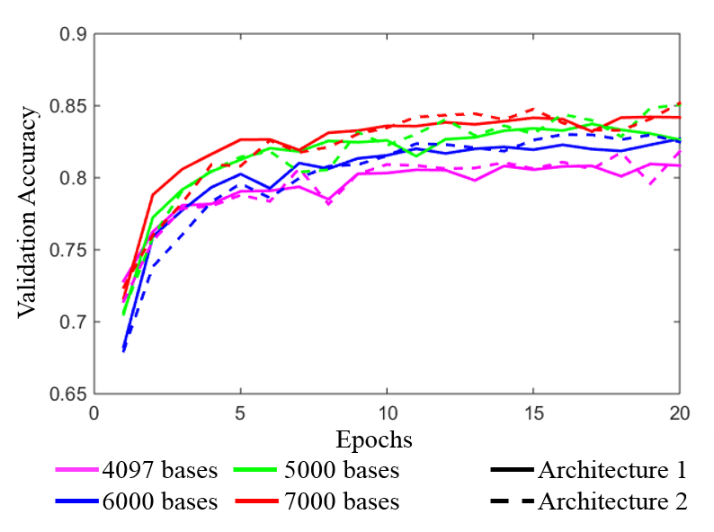


From these observations it can be seen that an higher training accuracy a has been obtained for the experiments where the number of basis has been set to 7000 for both subsets of data as well as both neural network architectures. The highest accuracy values obtained at the validation time is indicated in Table 1 and it can be seen that the recorded highest validation accuracy has been obtained for the experiments with 7000 bases. Furthermore when the results from two network architectures are analyzed it can be seen that the architecture 2 has yielded better training and validation accuracy values.
As the test data, we used 100k patch pairs from each of Liberty and Notredame datasets, which were not subjected to training. In order to evaluate our approach, we used the dictionary learnt for the Notredame dataset to encode the Liberty test dataset and used it as the input to the neural network trained for the Notredame dataset. Similarly we tested the Notredame test set using the Liberty dictionary and the trained model. The Receiver operating characteristic (ROC) curve related to the experiments are illustrated in Figure 9 and Figure 9 where the values of error@95% with related to different overcompleteness levels are indicated.
| Number of bases | Architecture 1 | Architecture 2 | ||
|---|---|---|---|---|
| Liberty dataset | Notredame dataset | Liberty dataset | Notredame dataset | |
| 4097 | 0.8096 | 0.6126 | 0.8175 | 0.6634 |
| 5000 | 0.8264 | 0.6669 | 0.8300 | 7605 |
| 6000 | 0.8373 | 0.7961 | 0.8506 | 0.8818 |
| 7000 | 0.8423 | 0.8357 | 0.8578 | 0.8970 |
| Training | Liberty | Notredame |
| Test | Notredame | Liberty |
| nSIFT + L2 | 22.53 | 29.84 |
| nSIFT + NNet | 14.35 | 20.44 |
| Trzcinski et al [24] | 14.15 | 18.05 |
| Brown et al [11] | - | 16.85 |
| Simonyan et al [25] | 9.88 | 16.56 |
| Han et al [4] | 3.87 | 6.90 |
| Zagoruyko and Komodakis [5] | 4.56 | 2.01 |
| Our method ( k = 4097, Architecture 1) | 13.52 | 16.17 |
| Our method ( k = 5000, Architecture 1) | 7.78 | 10.39 |
| Our method ( k = 6000,Architecture 1) | 4.26 | 5.69 |
| Our method ( k = 7000, Architecture 1) | 3.59 | 4.36 |
| Our method ( k = 4097, Architecture 2) | 9.69 | 12.11 |
| Our method ( k = 5000, Architecture 2) | 6.45 | 7.12 |
| Our method ( k = 6000, Architecture 2) | 3.19 | 4.13 |
| Our method ( k = 7000, Architecture 2) | 2.67 | 1.89 |
To compare our results with the previous approaches we used the evaluations carried out by the previous comparisons in the work by Han et al. [4] and in the work by Zagoruyko and Komodakis [5]. The obtain results are available in Table 2. The settings of the baseline methods used for the comparison are described in the following paragraph.
To compare SIFT feature’s [9] patch matching ability we used the same experimental results which have been obtained in [4]. They have used the SIFT features implemented by VL Feat [26] with the bin size of 16. Normalized SIFT (nSIFT) has been obtained by scaling the original SIFT feature such that its L2 norm is 1. In Table 2 the patch comparison based on nSIFT and L2 distance is denoted by nSIFT + L2. nSIFT + NNet stands for a framework where nSIFT features have been used as the input for a neural network with the 2 fully connected with 512 neurons in each. 150k iterations have been used to train this network. To compare the work by Trzcinski et al [24], Brown et al [11], Han et al [4] and Zagoruyko and Komodakis [5] we used their results which have been obtained under the best configuration.
When the results are compared it can be identified that our setting of using 7000 bases with the Architecture 2 has yielded better results when compared with the results obtained in the state-of-the-art methods [4, 5] for both datasets. Moreover when considering Liberty dataset, our setting with 6000 bases has outperformed the method by Zagoruyko and Komodakis [5] for the setting of 6000 bases with the Architecture 1 and Architecture 2 and for the setting with 7000 bases with Architecture 1. In addition for the Liberty dataset our setting with 6000 bases with Architecture 2 and 7000 bases with Architecture 1 has outformed the method by Han et al. [4]. When considering the Notredame dataset our method has outperformed the method by Han et al. [4] for the setting of 6000 bases with Architecture 1 and Architecture 2 and 7000 bases with Architecture 1 as well. From these results it can be observed that increasing overcompleteness has yeilded better results.
5 Conclusion
In this paper we have introduced and evaluated a novel patch descriptor by encoding patches using a dictionary and a neural network to compare the generated descriptor. To this end we studied two main neural network architectures and our model has outperformed the state-of-the-art accuracy on the standard UBC patch dataset. Among the architectures we suggest the architecture with one hidden layer which is shown to yield the best results. In contrast to previous patch descriptors which use visual information of the patch images, we use coefficients of sparse coding representation of the patch images capturing the statistical information in the patches . The use of neural network based patch comparison enables the technique to effectively match the obtained coefficient by capturing the non linear relationships across them. Furthermore we identified that increasing overcompleteness can result in better accuracy due to the fact that overcomplete representation is better able to capture the structures and patterns that are present in the original input image.
References
- [1] Yao, B., Bradski, G.,& Fei-Fei, L. (2012, June). A codebook-free and annotation-free approach for fine-grained image categorization. In Computer Vision and Pattern Recognition (CVPR), 2012 IEEE Conference on (pp. 3466-3473). IEEE.
- [2] Brown, M., & Lowe, D. G. (2007). Automatic panoramic image stitching using invariant features. International journal of computer vision, 74(1), 59-73.
- [3] Molton, N., Davison, A. J., & Reid, I. D. (2004, September). Locally Planar Patch Features for Real-Time Structure from Motion. In Bmvc (pp. 1-10).
- [4] Han, X., Leung, T., Jia, Y., Sukthankar, R., & Berg, A. C. (2015, June). Matchnet: Unifying feature and metric learning for patch-based matching. In Computer Vision and Pattern Recognition (CVPR), 2015 IEEE Conference on (pp. 3279-3286). IEEE.
- [5] Zagoruyko, S., & Komodakis, N. (2015, June). Learning to compare image patches via convolutional neural networks. In Computer Vision and Pattern Recognition (CVPR), 2015 IEEE Conference on (pp. 4353-4361). IEEE.
- [6] Field, D. J. (1994). What is the goal of sensory coding?. Neural computation, 6(4), 559-601.
- [7] Nakhmani, A., & Tannenbaum, A. (2013). A new distance measure based on generalized image normalized cross-correlation for robust video tracking and image recognition. Pattern recognition letters, 34(3), 315-321.
- [8] Bart, E., & Ullman, S. (2004, June). Class-based matching of object parts. In Computer Vision and Pattern Recognition Workshop, 2004. CVPRW’04. Conference on (pp. 173-173). IEEE.
- [9] Lowe, D. G. (2004). Distinctive image features from scale-invariant keypoints. International journal of computer vision, 60(2), 91-110.
- [10] Tola, E., Lepetit, V., & Fua, P. (2008, June). A fast local descriptor for dense matching. In Computer Vision and Pattern Recognition, 2008. CVPR 2008. IEEE Conference on (pp. 1-8). IEEE.
- [11] Brown, M., Hua, G., & Winder, S. (2011). Discriminative learning of local image descriptors. IEEE transactions on pattern analysis and machine intelligence, 33(1), 43-57.
- [12] Olshausen, B. A., & Field, D. J. (1997). Sparse coding with an overcomplete basis set: A strategy employed by V1?. Vision research, 37(23), 3311-3325.
- [13] Hyvärinen, A., & Hoyer, P. O. (2001). A two-layer sparse coding model learns simple and complex cell receptive fields and topography from natural images. Vision research, 41(18), 2413-2423.
- [14] Cai, D., Bao, H., & He, X. (2011, June). Sparse concept coding for visual analysis. In Computer Vision and Pattern Recognition (CVPR), 2011 IEEE Conference on (pp. 2905-2910). IEEE.
- [15] Perrault-Joncas, D., & Meila, M. (2014). Improved graph Laplacian via geometric self-consistency. arXiv preprint arXiv:1406.0118.
- [16] Belkin, M., & Niyogi, P. (2002). Laplacian eigenmaps and spectral techniques for embedding and clustering. In Advances in neural information processing systems (pp. 585-591).
- [17] Tenenbaum, J. B., De Silva, V., & Langford, J. C. (2000). A global geometric framework for nonlinear dimensionality reduction. science, 290(5500), 2319-2323.
- [18] Li, Y., Chen, J., Zhao, Y., & Lu, H. (2016, July). Adaptive affinity matrix for unsupervised metric learning. In Multimedia and Expo (ICME), 2016 IEEE International Conference on (pp. 1-6). IEEE.
- [19] Chung, F. R. (1997). Spectral graph theory (No. 92). American Mathematical Soc..
- [20] Efron, B., Hastie, T., Johnstone, I., & Tibshirani, R. (2004). Least angle regression. The Annals of statistics, 32(2), 407-499.
- [21] Kingma, D. P., & Ba, J. (2014). Adam: A method for stochastic optimization. arXiv preprint arXiv:1412.6980.
- [22] Yang, J., Yu, K., Gong, Y., & Huang, T. (2009, June). Linear spatial pyramid matching using sparse coding for image classification. In Computer Vision and Pattern Recognition, 2009. CVPR 2009. IEEE Conference on (pp. 1794-1801). IEEE.
- [23] Shang, L. (2008, September). Image reconstruction using a modified sparse coding technique. In International Conference on Intelligent Computing (pp. 220-226). Springer, Berlin, Heidelberg.
- [24] Trzcinski, T., Christoudias, M., Lepetit, V., & Fua, P. (2012). Learning image descriptors with the boosting-trick. In Advances in neural information processing systems (pp. 269-277).
- [25] Simonyan, K., Vedaldi, A., & Zisserman, A. (2014). Learning local feature descriptors using convex optimisation. IEEE Transactions on Pattern Analysis and Machine Intelligence, 36(8), 1573-1585.
- [26] Vedaldi, A., & Fulkerson, B. (2010, October). VLFeat: An open and portable library of computer vision algorithms. In Proceedings of the 18th ACM international conference on Multimedia (pp. 1469-1472). ACM.
- [27] Adiloglu, K., Annies, A., Wahlen, E., Purwins, H., & Obermayer, K. (2012). A graphical representation and dissimilarity measure for basic everyday sound events. IEEE Transactions on Audio, Speech, and Language Processing, 20(5), 1542-1552.
- [28] Scholler, S., & Purwins, H. (2011). Sparse approximations for drum sound classification. IEEE Journal of Selected Topics in Signal Processing, 5(5), 933-940.
- [29] Jia, Y., & Darrell, T. (2011). Heavy-tailed distances for gradient based image descriptors. In Advances in Neural Information Processing Systems (pp. 397-405).
- [30] Ballard, D. H., & Wixson, L. E. (1993, June). Object recognition using steerable filters at multiple scales. In Qualitative Vision, 1993., Proceedings of IEEE Workshop on (pp. 2-10). IEEE.
- [31] Ren, L., Shakhnarovich, G., Hodgins, J. K., Pfister, H., & Viola, P. (2005). Learning silhouette features for control of human motion. ACM Transactions on Graphics (ToG), 24(4), 1303-1331.
- [32] Lowe, D. G. (1999). Object recognition from local scale-invariant features. In Computer vision, 1999. The proceedings of the seventh IEEE international conference on (Vol. 2, pp. 1150-1157). IEEE.
- [33] Nowak, E., & Jurie, F. (2007, June). Learning visual similarity measures for comparing never seen objects. In Computer Vision and Pattern Recognition, 2007. CVPR’07. IEEE Conference on (pp. 1-8). IEEE.
- [34] Shakhnarovich, G. (2005). Learning task-specific similarity (Doctoral dissertation, Massachusetts Institute of Technology).
- [35] Tu, J. V. (1996). Advantages and disadvantages of using artificial neural networks versus logistic regression for predicting medical outcomes. Journal of clinical epidemiology, 49(11), 1225-1231.
- [36] O’Shea, K., & Nash, R. (2015). An introduction to convolutional neural networks. arXiv preprint arXiv:1511.08458.
- [37] Le, Q. V. (2015). A tutorial on deep learning part 2: autoencoders, convolutional neural networks and recurrent neural networks. Google Brain, 1-20.
- [38] Belongie, S., Malik, J., & Puzicha, J. (2002). Shape matching and object recognition using shape contexts. IEEE transactions on pattern analysis and machine intelligence, 24(4), 509-522.
- [39] Burl, M. C., Weber, M., & Perona, P. (1998, June). A probabilistic approach to object recognition using local photometry and global geometry. In European conference on computer vision (pp. 628-641). Springer, Berlin, Heidelberg.
- [40] Fergus, R., Perona, P., & Zisserman, A. (2003, June). Object class recognition by unsupervised scale-invariant learning. In Computer Vision and Pattern Recognition, 2003. Proceedings. 2003 IEEE Computer Society Conference on (Vol. 2, pp. II-II). IEEE.
- [41] Keysers, D., Deselaers, T., & Breuel, T. M. (2007). Optimal geometric matching for patch-based object detection. ELCVIA: electronic letters on computer vision and image analysis, 6(1), 44-54.