Hierarchical Clustering with Prior Knowledge
Abstract.
Hierarchical clustering is a class of algorithms that seeks to build a hierarchy of clusters. It has been the dominant approach to constructing embedded classification schemes since it outputs dendrograms, which capture the hierarchical relationship among members at all levels of granularity, simultaneously. Being greedy in the algorithmic sense, a hierarchical clustering partitions data at every step solely based on a similarity / dissimilarity measure. The clustering results oftentimes depend on not only the distribution of the underlying data, but also the choice of dissimilarity measure and the clustering algorithm. In this paper, we propose a method to incorporate prior domain knowledge about entity relationship into the hierarchical clustering. Specifically, we use a distance function in ultrametric space to encode the external ontological information. We show that popular linkage-based algorithms can faithfully recover the encoded structure. Similar to some regularized machine learning techniques, we add this distance as a penalty term to the original pairwise distance to regulate the final structure of the dendrogram. As a case study, we applied this method on real data in the building of a customer behavior based product taxonomy for an Amazon service, leveraging the information from a larger Amazon-wide browse structure. The method is useful when one want to leverage the relational information from external sources, or the data used to generate the distance matrix is noisy and sparse. Our work falls in the category of semi-supervised or constrained clustering.
Keywords:
hierarchical clustering, semi-supervised clustering, ultrametric distance, regularization1. Introduction
Hierarchical clustering is a a prominent class of clustering algorithms. It has been the dominant approach to constructing embedded classification schemes (Murtagh and Contreras, 2012). Compared with partition-based methods (flat clustering) such as K-means, a hierarchical clustering offers several advantages. First, there is no need to pre-specify the number of clusters. Hierarchical clustering outputs dendrogram (tree), which the user can then traverse to obtain the desired clustering. Second, the dendrogram structure provides a convenient way of exploring entity relationships at all levels of granularity. Because of that, for some applications such as taxonomy building, the dendrogram itself, not any clustering found in it, is the desired outcome. For example, hierarchical clustering has been widely employed and explored within the context of phylogenetics, which aims to discover the relationships among individual species, and reconstruct the tree of biological evolution. Furthermore, when dataset exhibits multi-scale structure, hierarchical clustering is able to generate a hierarchical partition of the data at different levels of granularity, while any standard partition-based algorithm will fail to capture the nested data structure.
In a typical hierarchical clustering problem, the input is a set of data points and a notion of dissimilarity between the points, which can also be represented as a weighted graph whose vertices are data points, and edge weights represent pairwise dissimilarities between the points. The output of the clustering is a dendrogram, a rooted tree where each leaf node represents a data point, and each internal node represents a cluster containing its descendant leaves. As the internal nodes get deeper in the tree, the points within the clusters become more similar to each other, and the clusters become more refined. Algorithms for hierarchical clustering generally fall into two types: Agglomerative (“bottom up”) approach: each observation starts in its own cluster, at every step a pair of most similar clusters are merged. Divisive (“top down”) approach: all observations start in one cluster, and splits are performed recursively, dividing a cluster into two clusters that will be further divided.
As a popular data analysis method, hierarchical clustering has been studied and used for decades. Despite its widespread use, it has rather been studied at a more procedural level in terms of practical algorithms. There are many hierarchical algorithms. Oftentimes, different algorithms produce dramatically different results on the same dataset. Compared with partition-based methods such as K-means and K-medians, hierarchical clustering has a relatively underdeveloped theoretical foundation. Very recently, Dasgupta (Dasgupta, 2015) introduced an objective function for hierarchical clustering, and justified it for several simple and canonical situations. A theoretical guarantee for this objective was further established (Moseley and Wang, 2017) on some of the widely used hierarchical clustering algorithms. Their works give insight into what those popular algorithms are optimizing for. Another route of theoretical research is to study the clustering schemes under an axiomatic view (Meilǎ, 2005; Carlsson and Mémoli, 2013; Eldridge et al., 2015; Zadeh and Ben-David, 2009; Ackerman et al., 2010; Ben-David and Ackerman, 2009), charactering different algorithms by the significant properties they satisfy. One of the influential works is Kleinberg’s impossibility theorem (Kleinberg, 2002), where he proposed three axioms for partitional clustering algorithms, namely scale-invariance, richness and consistency. He proved that no clustering function can simultaneously satisfy all three. It is showed (Carlsson and Memoli, 2010), however, if a nested family of partitions instead of fixed single partition is allowed, which is the case for hierarchical clustering, single linkage hierarchical clustering is the unique algorithm satisfying the properties. The stability and convergence theorems for single link algorithm are further established. Ackerman (Ackerman and Ben-David, 2016) proposed two more desirable properties, namely, locality and outer consistency, and showed that all linkage-based hierarchical algorithms satisfy the properties. Those property-based analyses provide a better understanding of the techniques, and guide users in choosing algorithms for their crucial tasks.
Based on similarity information alone, clustering is inherently an ill-posed problem where the goal is to partition the data into some unknown number of clusters so that within cluster similarity is maximized while between cluster similarity is minimized (Jain, 2010). It’s very hard for a clustering algorithm to recover the data partitions that satisfies various criteria of a concrete task. Therefore, any external or side information from other sources can be extremely useful in guiding clustering solutions. Clustering algorithms that leverage external information fall into the category of semi-supervised or constrained clustering (Basu et al., 2008). There are many ways to incorporate external information (Bair, 2013; Wagstaff et al., 2001; Liu et al., 2007; Xing et al., 1986). Starting from instance-level constraints such as must-link constraints and cannot-link constraints, many approaches try to modify the objective function of the algorithms to incorporate pairwise constraints. Beyond pairwise constraints, external knowledge has been used as the seeds for clustering, cluster size constraints, or as prior probabilities of cluster assignment. However, the majority of existing semi-supervised clustering methods are based on partition-based clustering. Comparatively few methods on hierarchical clustering have been proposed. In fact, human is very good at summarizing and extracting high level relational information between entities. Human built taxonomies, such as WordNet, Wikipedia, 20 newsgroup dataset etc. are high quality sources of ontological information that a hierarchical clustering algorithm can leverage. Several factors contributed to the underdevelopment in the semi-supervised hierarchical clustering algorithms. One is the lack of global objective functions. Only very recently an objective function for hierarchical clustering was proposed (Dasgupta, 2015). Another reason is that simple must-link and cannot-link constraints used in flat clustering are not suitable in hierarchical clustering since entities are linked at different level of granularity. Furthermore, the output of hierarchical clustering is a dendrogram which is harder to represent than the result from a flat clustering.
In this paper, we focus on agglomerative hierarchical clustering algorithms since divisive algorithms can be considered as a repeated partitional clustering (bisectioning). We describe a method of incorporating prior ontological knowledge into agglomerative hierarchical clustering by using a distance function in ultrametric space representing the complete or partial tree structure. The constructed ultrametic distance is combined with the original task-specific distance to form a new distance measure between the data points. The weight between the two distance components, which reflects the confidence of prior knowledge, is a hyper-parameter that can be tuned in a cross-validation manner, by optimizing an external task-specific metric. We then use a property-based approach to select algorithms to solve the semi-supervised clustering problem. We note that there are several pioneer works on constrained hierarchical clustering (Huang and Ribeiro, 2016; Heller and Ghahramani, 2005; Bade and Nürnberger, 2007; Jose, 2000). Davidson (Davidson and Ravi, 2005) explored the feasibility problem of incorporating 4 different instance and cluster level constraints into hierarchical clustering. Zhao (Zhao and Qi, 2010) studied hierarchical clustering with order constraints in order to capture the ontological information. Zheng (Zheng and Li, 2011) represented triple-wise relative constraints in a matrix form, and obtained the ultrametric representation by solving a constrained optimization problem. Compared with previous studies, our goal is to recover the hierarchical structure of the data which resembles existing ontology and yet provides new insight into entity relationships based on a task-specific distance measure. The external ontological knowledge serves as soft constraints in our approach, which is different from the hard constraints used in the previous works. Our constructed distance measure also fits naturally with the global object function (Dasgupta, 2015) recently proposed for hierarchical clustering.
The paper is organized as follows: In Section 2, we state the problem and introduce the concepts used in this paper. In Section 3, we discuss our approach to solving the semi-supervised hierarchical clustering problem. In Section 4, we present a case study of applying the proposed method on real data to the building of a customer behavior based product taxonomy for an Amazon service. Finally, we summarize the results in Section 5.
2. Problem Setting
In this section we define the context and the problem we want to solve, i.e. the semi-supervised hierarchical clustering problem.
Given a set of data points , a pairwise dissimilarity measure , a task-specific performance measure , and a complete or partial tree structure contains external ontological information, whose leaf nodes are instances of , and whose internal nodes are clusters containing descendant leaves. The goal of the semi-supervised hierarchical clustering problem is to output a dendrogram over represented as a pair , where is the set of data points, , is a partition of , such that the dendrogram resembles and performs best in terms of .
Two important concepts related to the above problem setting are the notion of dissimilarity and the dendrogram.
Definition 2.1.
A dissimilarity measure is usually represented as a pair , where X is a set, and such that for any :
| , non-negativity | |||
| if and only if , identity | |||
| , symmetry |
As an example, cosine dissimilarity is a commonly used dissimilarity measure in high-dimensional positive space.
Definition 2.2.
If the dissimilarity also satisfies the following triangle inequality, for any :
| (1) |
then we have a distance measurement in the metric space.
Euclidean distance and manhattan distance are popular metric space distances.
Definition 2.3.
A dendrogram is a tree that satisfies the following conditions (Carlsson and Memoli, 2010):
| There exists such that contains only one cluster for . | |||
| If , then refines | |||
| For all , there exists such that for . |
Condition 1 ensures that the initial partition is the finest possible, each data point forms a cluster. Condition 2 tells that for large enough , the partition becomes trivial. The whole space is one cluster. Condition 3 ensures that the structure of dendrogram is nested. Condition 4 requires that the partition is stable under small perturbation of size . The parameter of dendrogram is a measure of scale, and reflected in the height of different levels. The notion of resemblance between dendrograms will be discussed more in Section 3.3.
3. Proposed Method
In order to incorporate prior knowledge into hierarchical clustering, we need a way to faithfully represent prior relational information between entities. Since relational knowledge such as hyponymy and synonymy relations in WordNet, class taxonomy in the 20-newsgroups dataset can usually be represented as a tree, this suggests that it is convenient to define a distance function that leverages the tree structure. In fact, Resnik’s approach (arXiv preprint Cmp-lg/9511007 and undefined 1995, [n. d.]) to semantic similarity between words was the first attempt to brings together the ontological information in WordNet with the corpus information. Figure 1 shows a fragment of structured lexicons defined in WordNet.

To encode a tree structure, we first introduce the concept of ultrametric space.
Definition 3.1.
A metric space is an ultrametric if and only if,
| (2) |
The ultrametric condition requires that every triangle formed by any three data points has to be an acute isosceles triangle, which is a stronger condition than the triangle inequality in Equation 1.
It is well known that a dendrograms can be represented as ultrametrics. The relationship between dendrograms and ultrametric has been discussed in several works (Roy and Pokutta, 2016; Jardine and Sibson, 1971; Hartigan, 1985; Jain and Dubes, 1988). The equivalence between dendrograms and ultrametrics was further established by Carlsson in (Carlsson and Memoli, 2010). A hierarchical clustering algorithm essentially outputs a map from finite metric space into finite ultrametric space .
3.1. An ultrametic function to encode prior relational information
We now propose an ultrametric distance function to encode the tree structure between entities.
Definition 3.2.
Let be a rooted tree of entity relationship. For any node in , let be a subtree rooted at , be the leaves of the subtree, and be the number of leaf nodes. For any leaf node , the expression denotes their lowest common ancestor in T. We define a distance function between any leaf node as follows:
| (3) |
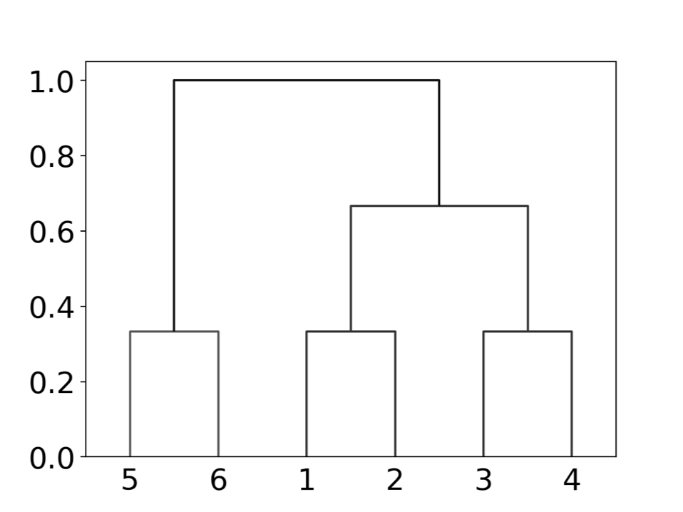
In the above definition, is the total number of leaf nodes in the tree . It is a normalization constant to ensure the distance is between . As an example, Figure 2 shows a small tree consisting of leaf nodes. According to Definition 3.2, the distances between pairs are and , respectively. Although the tree structure in Figure 2 doesn’t specify the exact distance values, it encodes the hierarchical relations between data points. It is easy to see that point is more similar to point than to point or .

Lemma 3.3.
The distance function defined in Definition 3.2 is an ultrametric.
Proof.
For any leaf node in , is either in the subtree or not in the subtree . If is in the subtree , then . If is not in the subtree , we have , then . Therefore, in either case, . ∎
Because of the equivalence between dendrograms and ultrametrics, once we encode the tree using an ultrametric distance, there is a unique dendrogram corresponding to it.
A pairwise distance function quantifies the dissimlarity between any pair of points. However, it doesn’t define the distance between clusters of points.
Linkage-based hierarchical clustering algorithms calculate distance between clusters based on different heuristics. Let be a linkage function that assigns a non-negative value to each pair of non-empty clusters based on a pairwise distance function . Some choices of linkage functions are:
| , single linkage | |||
| , complete linkage | |||
| , average linkage |
All three linkage functions lead to a popular hierarchical clustering algorithm. However, it is known that the results from average link and complete link algorithms depend on the ordering of points, while single link is exempted from this undesirable feature. The cause lies in the way that an algorithm deals with situation when more than two points are equally good candidates for merging next. Since we merge the data points two at a time, then the merge order will determine the final structure of the dendrogram. However, it can be shown that when an ultrametric distance is used, all three linkage-based algorithms will output the same dendrogram.
Theorem 3.4.
The dendrogram structure from a complete linkage or average linkage hierarchical algorithm is independent of the merge order of equally good candidates when the distance measure is an ultrametric. (The proof is in Appendix A.)
As an example, for the small tree defined in Figure 2 and the distance function defined in Equation 3, all three linkage-based algorithms produce the same dendrogram presented in Figure 3. The dendrogram faithfully encodes all the grouping relations between leaf nodes from the original tree.
3.2. Combine the two distance components
To incorporate the external ontological information into the hierarchical clustering, we combine the as-defined ultrametric distance function with the problem-specific distance measure using a weighted sum of the two components. Let be the problem-specific distance (we normalize it so that its value is between ), and be the ultrametric distance encoding the prior ontological knowledge. The new distance function to be fed into a hierarchical clustering algorithm can be constructed as follows:
| (4) |
Similar to some regularized machine learning techniques, the ultrametric distance is added as a penalty term to the original pairwise distance. When , we go back to the unregulated hierarchical clustering case, in which only the problem-specific distance is used. When , we recover the relational structure from the external source. Essentially, measures the minimal effort that a hierarchical clustering algorithm needs to make in order to join and . The hyper-parameter determines the proportion that the prior knowledge contribute to the clustering. It reflects our confidence in each component. Since the ultrametric term is added pair-wisely, the new distance function fits naturally with the global object function proposed in (Dasgupta, 2015). In that context, the ultrametic term is a soft constraint added to the object function.
The tuning of the hyper-parameter can be achieved in different ways depending on the availability of external labels or performance metric. Without external gold standard, the tuning can be conducted by maximizing some internal quality measures such as Davies-Bouldin index or Dunn index. With the availability of external labels, parameter can be tuned in a cross-validation manner. Various performance measures have been proposed to evaluate clustering results given a gold standard (Zhao et al., [n. d.]). It should be noted that some performance metrics require conversion of a dendrogram into a flat partition. In those cases, the number of the clusters is also hyper-parameter to tune. If the dendrogram itself, not any clustering found in it, is the desired outcome, we can aggregate the performance metric across different for a given , and choose the dendrogram corresponding to the with the best overall performance.
3.3. Property based approach for clustering algorithm selection
In Equation 4, the overall distance function is no longer ultrametric if the problem-specific distance is not ultrametric. To remediate the problem, one could convert the problem-specific distance function into an ultrametric distance. However, finding the closest ultrametric to a noisy metric data is -complete. We also need to specify a measure of distortion between the original metric and the approximated ultrametric (Di Summa et al., 2015). One could also try to feed the problem-specific distance into a hierarchical clustering algorithm, and let the algorithm output an ultrametric for us. In fact, it is shown in (Carlsson and Memoli, 2010) that single linkage hierarchical clustering produces ultrametric outputs exactly as those from a maximal sub-dominant ultrametric construction, which is a canonical construction from metric to ultrametric.
In addition to the above property, single linkage algorithm also enjoys other properties that are important to applications such as taxonomy building. In (Ackerman and Ben-David, 2016), Ackerman shows that all linkage-based hierarchical algorithms satisfying the locality and outer consistency properties. However, it is observed that both complete linkage and average linkage are not stable under small perturbation, and not invariant under permutation of data label (Carlsson and Memoli, 2010). It is shown that only single linkage algorithm is stable in the Gromov-Hausdorff sense and has nice convergence property (Eldridge et al., 2015) . Gromov-Hausdorff distance measures how far two finite spaces are from being isometric. The stability property is critical to our distance function defined in Equation 4 since we’d like a continuous map from metric spaces into dendrograms as we change the hyper-parameter . Based on the stability property, we can define the structure resemblance discussed in the problem statement Section 2. We’d like the dendrogram from our semi-supervised method to be similar to the dendrogram encoding prior domain knowledge as measured by Gromov-Hausdorff distance. It can be shown that for two dendrograms generated from single linkage algorithm defined on the same data set , their Gromov-Hausdorff distance is bounded above by the norm of the difference between two underlying metric spaces .
One drawback of single linkage algorithm is that it is not sensitive to variations in the data density, which can cause “chaining effect”. However, we believe that this “chaining effect”is alleviated in our semi-supervised approach since we use a prior tree to regulate the dendrogram structure from clustering. Based on the above reasons, we choose to use single linkage algorithm to solve our semi-supervised hierarchical clustering problem.
3.4. Computational complexity
All agglomerative hierarchical clustering methods need to compute the distance between all pairs in the dataset. The complexity of this step, in general, is , where is the number of data points. In each of the subsequent merging iterations, the algorithm needs to compute the distance between the most recently created cluster and all other existing clusters. Therefore, the overall complexity is if implemented naively. If done more cleverly, the complexity can be reduced to .
In our approach, the most computationally expensive step is the calculation of pairwise ultrametric distance based on Equation 3 since it requires finding the lowest common ancestor of two leaf nodes within a tree. The complexity of finding the lowest common ancestor is , where is the height of the tree (length of longest path from a leaf to the root). In the worst case is equivalent to , but if the tree is balanced, can be achieved. It also requires space. Fast algorithm exists that can provide constant-time queries of lowest common ancestor by first processing a tree in linear time.
For large datasets, one way to speed up the computation is pre-cluster the data points into clusters by either leveraging external ontological information (cutting the tree at high levels) or by using a partition-based clustering algorithm. Each of the clusters is then treated separately, and single-link hierarchical clustering algorithm is employed to build a dendrogram for each sub-cluster. Finally, the dendrograms are combined into one dendrogram by applying single-link algorithm which treats each of the dendrograms as an internal node. The overall complexity in this case is . For reasonably large , the computation time can be greatly reduced. Within each sub-cluster, the search for optimal is conducted in a cross-validation manner by evaluating a task-specific metric. The full algorithm including hyper-parameter tuning is presented in Algorithm 1.
4. Case Study: A Customer Behavior Based Product Taxonomy
In this session, we apply the proposed method to the construction of a customer behavior based product taxonomy for an Amazon service. The goal here is to build a taxonomy that captures substitution effects among different products and product groups.
To achieve this goal, we could define a dissimilarity measure between products based on a customer behavior metric, and group products using a hierarchical clustering algorithm. However, due to the huge size of Amazon selection and customer base, customer behavior data is usually sparse and noisy. Furthermore, for taxonomy building purpose, we’d like the grouping to be consistent across all levels, and the resulting hierarchy to be logical as perceived by a human reader. As discussed in the introduction, clustering with only a dissimilarity measure is an ill-posed problem. It’s hard for a clustering algorithm to recover the data partitions that satisfies various criteria of a concrete task. On the other hand, human-designed taxonomies usually perform well in terms of consistency and human readability. In this work, we employ a semi-supervised approach for the building of a product taxonomy, leveraging the ontological information from existing Amazon-wide browse hierarchy.
4.1. Amazon browse hierarchy
Amazon Browse enables customers’ discovery experience by organizing Amazon’s product selection into a discovery taxonomy. The browse hierarchy is loaded every time a customer visits Amazon website. The leaf nodes of Amazon browse hierarchy represent a group of products of the same type such as coffee-mug, dvd-player etc. The internal nodes represent higher levels of product groupings. While being important in influencing customer searches, Amazon browse trees are not built to reflect program-specific product substitution effects. They determines what customer see but not their following decisions after seeing the search results.
4.2. Customer behavior based dissimilarity measure
To construct a customer behavior based dissimilarity measurement between leaf nodes, we first use Latent Dirichlet Allocation (LDA) (Blei et al., 2003; Blei David, Carin Lawrence, 2010) to obtain an embedding for each leaf node based on customers’ click, cart-add and purchase actions for the Amazon service. To apply LDA to customer searches, we treat each search keyword as a document, and each leaf node as a word in the vocabulary. Each element in the document-word matrix stores the frequency of certain customer actions such as clicks, cart-adds, purchases performed on a particular leaf node within the context that customer search for a given keyword. Provided with the number of topics, LDA outputs the probability of word appears in each topic. We use the vector of topic probabilities for each leaf node as the embedding. LDA essentially is used here as a dimensionality reduction method similar to matrix factorization.
We then calculate the cosine dissimilarity between pairs of leaf nodes using the embeddings. Since each element in the embedding is a probability, a positive number, the cosine dissimilarity is between and . The cosine dissimilarity between two leaf nodes and , is calculated as:
| (5) |
4.3. Hyper-parameter tuning by maximizing the performance of substitution group
Given the problem-specific distance measure, and the ultrametric distance encoding Amazon browse node hierarchy, we can combine the two components to form the new distance measure in our semi-supervised hierarchical clustering problem. As discussed in section 3, the weighting parameter can be tuned in a cross-validation manner by optimizing a task-specific performance metric.

For evaluation, we optimize the performance of using the resulting clusters as substitution groups, within which products are substitutable with each other. It’s reasonable to assume that customers who search for the same keyword share similar type of demand. If all the customers search for the same keyword end up purchasing items from the same substitution group, then our definition of the substitution group captures all the substitution effect for that demand. If customers search for the same keyword end up purchasing items from the many different substitution groups, then our grouping of products does a poor job in capturing product substitution. Based on the above rationale, we define three metrics to capture of the substitution performance. “Purity”, which is defined as the average percentage of customer purchases falling within the top substitution group for each search keyword. “Entropy”, for each search keyword, there is a categorical distribution of customer purchases from different substitution groups. The average entropy of the categorical distribution for each search keyword defines the entropy metric. “Weighted entropy”, this metric is similar to the Entropy metric except that each keyword is weighted by the number of customer purchases. For Purity metric, high values are preferred. For Entropy metrics, low values are better.
Based on the performance metrics, our experiment was conducted as follows: A full month of customers’ search data was used as the training data to obtain the LDA embedding for the leaf nodes. A grid search of hyper-parameter and the number of clusters was conducted using cross-validation on the data from the first half of the following month. Figure 4 shows the cross-validation result as a heat map of the normalized purity metric. The lighter the color, the higher the purity. Due to the discrete nature of the tree structure, certain numbers of flat clusters can not be formed from the dendrograms. Those cases are shown as black squares in the heatmap. As we can see from the figure, our semi-supervised approach achieves consistently better performance than both the pure customer behavior based dissimilarity and pure browse taxonomy . Similar trends can be observed for entropy-based metrics (not shown in this paper). It can be noted from the figure that using the pure browse structure based taxonomy is not flexible in terms of number of clusters. By mixing the two distance components, we can create hierarchy of leaf nodes at different levels of granularity. Based on the cross-validation result, we select the best and test it on the data from the second half of the month. The test result is presented in Table 1. To facilitate the comparison with pure browse node based taxonomy, we choose the cluster numbers of 46 and 69 for testing. As we can see from the table, the semi-supervised approach performs best during the testing period across all three metrics (highest in Purity, lowest in Entropy metrics).
| Clusters | Purity | Entropy | Weighted Entropy | |
|---|---|---|---|---|
| 46 | 0.0 | 0.93 | 1.0 | 1.0 |
| 46 | 0.85 | 1.0 | 0.68 | 0.72 |
| 46 | 1.0 | 0.96 | 0.72 | 0.80 |
| 69 | 0.0 | 0.92 | 1.0 | 1.0 |
| 69 | 0.7 | 1.0 | 0.69 | 0.71 |
| 69 | 1.0 | 0.96 | 0.77 | 0.79 |
Figure 5 presents the evolution of dendrogram structure for the segment of “Coffee, Tea and Cocoa”. As we decrease (increase mixing), one can observe mixing of coffee and tea at lower level of the dendrograms, which reflects a notion of substitution between the two product groups. In another example, figure 6 presents the dendrogram evolution for Beans, Grains and Rice segment. In that case, we can observe a finer grouping of products within either rice group or beans group as we decrease . However, products from different groups don’t mix, which means the substitution effect is not as significant as that between Coffee and Tea products.


5. Conclusion
Hierarchical clustering is a a prominent class of clustering algorithms. It has been the dominant approach to constructing embedded classification schemes. In this paper, we propose a novel method of incorporating prior domain knowledge about entity relations into hierarchical clustering. By encoding the prior relational information using an ultrametric distance function, we have shown that the popular linkage based hierarchical clustering algorithms can faithfully recover the prior relational structure between entities. We construct the semi-supervised clustering problem by applying the ultrametric distance as a penalty term to the original task-specific distance measure. We choose to use single link algorithm to solve the problem due to its favorable stability and convergence properties. As an example, we apply the proposed method to the construction of a customer behavior based product taxonomy for an Amazon service leveraging an Amazon-wide browse structure. Our experiment results show that the semi-supervised approach achieves better performance than the clustering purely based on task-specific distance and the clustering purely based on external ontological structure.
Appendix A Complete linkage hierarchical clustering with ultrametric distance
It is known that in a metric space, when there are two or more equally good candidates for merging at a certain step, the results from complete link hierarchical clustering algorithms depend on the ordering of merging. In this section, we show that if the distance function is ultrametric, the dendrogram structure from complete linkage does not depend on the merging order.
Proof.
We first show under complete link and ultrametric assumptions, the ultrametric condition also holds among clusters. Let represent three disjoint clusters (can be singletons), we want to show .
Under complete linkage, without loss of generality, we assume , and
| (6) | ||||
Then we have,
| (7) | ||||
We now show for any disjoint clusters , if at a certain stage are smaller than other cluster-cluster distances, which means and are equally good candidates for merge next. Regardless of merging order between and , cluster will always merge last.
In fact, due to ultrametric condition, if , then . It means will merge before or . Then, there is no ambiguity about merging order. merges first, then . will always merge last to the cluster. ∎
In a similar manner, we can show the same result for average link hierarchical clustering with ultrametric distance.
References
- Ackerman and Ben-David (2016) Margareta Ackerman and Shai Ben-David. 2016. A Characterization of Linkage-Based Hierarchical Clustering. Journal of Machine Learning Research 17 (2016), 1–17.
- Ackerman et al. (2010) Margareta Ackerman, Shai Ben-David, and David Loker. 2010. Towards Property-Based Classification of Clustering Paradigms. Nips 2010 (2010), 1–9. https://papers.nips.cc/paper/4101-towards-property-based-classification-of-clustering-paradigms.pdf
- arXiv preprint Cmp-lg/9511007 and undefined 1995 ([n. d.]) P Resnik arXiv preprint Cmp-lg/9511007 and undefined 1995. [n. d.]. Using information content to evaluate semantic similarity in a taxonomy. arxiv.org ([n. d.]). https://arxiv.org/abs/cmp-lg/9511007
- Bade and Nürnberger (2007) Korinna Bade and Andreas Nürnberger. 2007. Personalized hierarchical clustering. Proceedings - 2006 IEEE/WIC/ACM International Conference on Web Intelligence (WI 2006 Main Conference Proceedings), WI’06 June (2007), 181–187. https://doi.org/10.1109/WI.2006.131
- Bair (2013) Eric Bair. 2013. Semi-supervised clustering methods. (2013), 1–28. https://doi.org/10.1002/wics.1270 arXiv:1307.0252
- Basu et al. (2008) Sugato Basu, Ian Davidson, and Kiri Wagstaff. 2008. Constrained Clustering: Advances in Algorithms, Theory, and Applications, 1 edition. Vol. 45. 961–970 pages. https://doi.org/10.1007/BF02884971
- Ben-David and Ackerman (2009) Shai Ben-David and Margareta Ackerman. 2009. Measures of Clustering Quality: A Working Set of Axioms for Clustering. Advances in Neural Information Processing Systems 21 (2009), 121–128. http://books.nips.cc/nips21.html
- Blei et al. (2003) David M Blei, Andrew Y Ng, and Michael I Jordan. 2003. Latent Dirichlet Allocation. J. Mlr 3 (2003), 993–1022.
- Blei David, Carin Lawrence (2010) Dunson David Blei David, Carin Lawrence. 2010. Probabilistic Topic Models. IEEE Signal Processing Magazine 27, 6 (2010), 55–65. https://doi.org/10.1109/MSP.2010.938079 arXiv:1003.4916
- Carlsson and Memoli (2010) G Carlsson and F Memoli. 2010. Characterization, Stability and Convergence of Hierarchical Clustering Methods. Journal of Machine Learning Research 11 (2010), 1425–1470.
- Carlsson and Mémoli (2013) Gunnar Carlsson and Facundo Mémoli. 2013. Classifying Clustering Schemes. Foundations of Computational Mathematics 13, 2 (2013), 221–252. https://doi.org/10.1007/s10208-012-9141-9 arXiv:1011.5270
- Dasgupta (2015) Sanjoy Dasgupta. 2015. A cost function for similarity-based hierarchical clustering. Section 2 (2015), 1–18. https://doi.org/10.1145/2897518.2897527 arXiv:1510.05043
- Davidson and Ravi (2005) Ian Davidson and S S Ravi. 2005. Agglomerative Hierarchical Clustering with Constraints: Theory and Empirical Resutls. 9th European Conference on Principles and Practice of Knowledge Discovery in Databases, PKDD 2005 (2005), 59–70. http://citeseerx.ist.psu.edu/viewdoc/download?doi=10.1.1.62.2314{&}rep=rep1{&}type=pdf
- Di Summa et al. (2015) Marco Di Summa, David Pritchard, and Laura Sanità. 2015. Finding the closest ultrametric. Discrete Applied Mathematics 180 (2015), 70–80. https://doi.org/10.1016/j.dam.2014.07.023
- Eldridge et al. (2015) Justin Eldridge, Mikhail Belkin, and Yusu Wang. 2015. Beyond Hartigan Consistency: Merge Distortion Metric for Hierarchical Clustering. 40, 1981 (2015), 1–19. arXiv:1506.06422 http://arxiv.org/abs/1506.06422
- Hartigan (1985) J. A. Hartigan. 1985. Statistical theory in clustering. Journal of Classification 2, 1 (dec 1985), 63–76. https://doi.org/10.1007/BF01908064
- Heller and Ghahramani (2005) Katherine a. Heller and Zoubin Ghahramani. 2005. Bayesian hierarchical clustering. Proceedings of the 22nd international conference on Machine learning (2005), 297–304. https://doi.org/10.1145/1102351.1102389
- Huang and Ribeiro (2016) Weiyu Huang and Alejandro Ribeiro. 2016. Hierarchical Clustering Given Confidence Intervals of Metric Distances. (2016), 1–13. arXiv:1610.04274 http://arxiv.org/abs/1610.04274
- Jain (2010) Anil K Jain. 2010. Data Clustering: 50 Years Beyond K-Means. 19th International Conference in Pattern Recognition (ICPR) (2010), 651–666. https://doi.org/10.1016/j.patrec.2009.09.011
- Jain and Dubes (1988) Anil K. Jain and Richard C. Dubes. 1988. Algorithms for clustering data. Prentice Hall. 320 pages. https://dl.acm.org/citation.cfm?id=46712
- Jardine and Sibson (1971) Nicholas. Jardine and Robin Sibson. 1971. Mathematical taxonomy. Wiley. 286 pages. https://books.google.com/books/about/Mathematical{_}Taxonomy.html?id=ka4KAQAAIAAJ
- Jose (2000) San Jose. 2000. Model-Based Hierarchical Clustering. (2000), 599–608.
- Kleinberg (2002) Jon Kleinberg. 2002. An impossibility theorem for clustering. Advances in Neural Information Processing Systems (2002), 446–453. https://doi.org/10.1103/PhysRevE.90.062813 arXiv:arXiv:physics/0607100v2
- Liu et al. (2007) Yi Liu, Rong Jin, and Anil K Jain. 2007. BoostCluster: boosting clustering by pairwise constraints. Proceedings of the 13th {ACM} {SIGKDD} international conference on Knowledge discovery and data mining (2007), 450–459. https://doi.org/10.1145/1281192.1281242
- Meilǎ (2005) Marina Meilǎ. 2005. Comparing clusterings. Proceedings of the 22nd international conference on Machine learning - ICML ’05 (2005), 577–584. https://doi.org/10.1145/1102351.1102424
- Moseley and Wang (2017) Benjamin Moseley and Joshua R Wang. 2017. Approximation Bounds for Hierarchical Clustering: Average Linkage, Bisecting K-means, and Local Search. Nips Nips (2017).
- Murtagh and Contreras (2012) Fionn Murtagh and Pedro Contreras. 2012. Algorithms for hierarchical clustering: An overview. Wiley Interdisciplinary Reviews: Data Mining and Knowledge Discovery 2, 1 (2012), 86–97. https://doi.org/10.1002/widm.53 arXiv:1105.0121
- Roy and Pokutta (2016) Aurko Roy and Sebastian Pokutta. 2016. Hierarchical Clustering via Spreading Metrics. (2016), 1–35. arXiv:1610.09269 http://arxiv.org/abs/1610.09269
- Wagstaff et al. (2001) Kiri Wagstaff, Claire Cardie, Seth Rogers, and Stefan Schroedl. 2001. Constrained K-means Clustering with Background Knowledge. International Conference on Machine Learning (2001), 577–584. https://doi.org/10.1109/TPAMI.2002.1017616
- Xing et al. (1986) Eric P Xing, Andrew Y Ng, Michael I Jordan, and Stuart Russell. 1986. Distance metric learning, with application to clustering with side-information. Transportation Research Record (1986).
- Zadeh and Ben-David (2009) RB Zadeh and S Ben-David. 2009. A uniqueness theorem for clustering Clustering. Proceedings of the twenty-fifth conference on (2009).
- Zhao and Qi (2010) Haifeng Zhao and Zi Jie Qi. 2010. Hierarchical agglomerative clustering with ordering constraints. 3rd International Conference on Knowledge Discovery and Data Mining, WKDD 2010 (2010), 195–199. https://doi.org/10.1109/WKDD.2010.123
- Zhao et al. ([n. d.]) Y Zhao, G Karypis of the eleventh international conference on …, and undefined 2002. [n. d.]. Evaluation of hierarchical clustering algorithms for document datasets. dl.acm.org ([n. d.]). https://dl.acm.org/citation.cfm?id=584877
- Zheng and Li (2011) Li Zheng and Tao Li. 2011. Semi-supervised hierarchical clustering. Proceedings - IEEE International Conference on Data Mining, ICDM (2011), 982–991. https://doi.org/10.1109/ICDM.2011.130