Cooper instability generated by attractive fermion-fermion interaction in the two-dimensional semi-Dirac semimetals

Yao-Ming Dong Affiliation: Department of Physics, Tianjin University, Tianjin 300072, P.R. China Dong-Xing Zheng Affiliation: Department of Physics, Tianjin University, Tianjin 300072, P.R. China Jing Wang Affiliation: Corresponding author: jing

\textunderscore

wang@tju.edu.cn Affiliation: Department of Physics, Tianjin University, Tianjin 300072, P.R. China Affiliation: Department of Modern Physics, University of Science and Technology of China, Hefei, Anhui 230026, P.R. China

August 24, 2026

Abstract

Cooper instability associated with superconductivity in the two-dimensional semi-Dirac semimetals is attentively studied in the presence of attractive Cooper-pairing interaction, which is the projection of an attractive fermion-fermion interaction. Performing the standard renormalization group analysis shows that the Cooper theorem is violated at zero chemical potential but instead Cooper instability can be generated only if the absolute strength of fermion-fermion coupling exceeds certain critical value and transfer momentum is restricted to a confined region, which is determined by the initial conditions. Rather, the Cooper theorem would be instantly restored once a finite chemical potential is introduced and thus a chemical potential-tuned phase transition is expected. Additionally, we briefly examine the effects of impurity scatterings on the Cooper instability at zero chemical potential, which in principle are harmful to Cooper instability although they can enhance the density of states of systems. Furthermore, the influence of competition between a finite chemical potential and impurities upon the Cooper instability is also simply investigated. These results are expected to provide instructive clues for exploring unconventional superconductors in the kinds of semimetals.

pacs

74.20.Fg, 74.40.Kb,64.60.-i,74.62.En

I Introduction

Accompanying with the remarkable developments in the Dirac fermions [4, 1, 5, 6, 7, 2, 3, 8, 9, 10, 11, 12, 13, 17, 14, 15, 16, 18, 19, 20, 21, 22, 23, 24] that own a number of discrete Dirac points and a linear dispersion in two or three directions irrespective of their microscopic details [1, 2, 3, 13, 14, 15, 16], the two-dimensional (2D) semi-Dirac (SD) electronic semimetals, one cousin of Dirac-like family, have recently been attracting many studies [28, 31, 29, 30, 32, 34, 33, 25, 26, 27, 38, 39, 35, 36, 37, 42, 40, 41, 43] attesting to the unique dispersion around their Dirac points, namely parabolic in one direction and linear in the other. To be concrete, they were widely presented in distinct circumstances, for instance, the quasi-two dimensional organic conductor $\alpha-(\mathrm{BEDT-TTF)_{2}I_{3}}$ salt under uniaxial pressure [29], tight-binding honeycomb lattices for the presence of a magnetic field [30], and the $\mathrm{VO_{2}-TiO_{2}}$ multilayer systems (nanoheterostructures) [31] as well as photonic systems consisting of a square array of elliptical dielectric cylinders [27]. In principle, there are at least three major ingredients, which are expected to be intimately associated with the low-energy fates of physical properties of fermionic systems, for instance the ground states, transport quantities and so on [49, 46, 47, 1, 48, 2, 45, 3, 44]. Specifically, the first ingredient is the dispersion of low-energy excitations and the second one is the kind of fermion-fermion interactions that glues these low-energy excitations. Lastly, the potential impurity scattering serves as the third ingredient, which is always present in real systems.

It is therefore of considerable significance to explore how these physical facets influence the low-energy properties of 2D SD materials. One of the most interesting phenomena is the development of superconductivity. The well-known Bardeen-Cooper-Schrieffer (BCS) theory [50] tells us that an arbitrarily weak attractive force can glue a pair of electrons and induce the Cooper pairing instability in normal metals, which is directly linked to the superconductivity. This process can be expressed alternatively by virtue of the language of modern renormalization group theory, namely the absolute strength of attractive interaction is (marginally) relevant with respect to the corresponding effective model, which eventually runs to the strong (infinite) coupling no matter how small its starting value is [52, 53, 51]. Recently, the Cooper pairing of Dirac fermions, in particular intrinsic Dirac semimetals, has been paid a multitude of attentions [1, 56, 57, 64, 58, 59, 60, 61, 62, 63, 54, 55]. One of the most important points addressed by previous works is that the Cooper pairing only forms once the absolute value of attractive interaction exceeds certain critical value owing to the vanishing density of states (DOS) and linear dispersions at the Dirac points of Dirac semimetals (DSM). This implies the Cooper theorem does not work and there may exist some quantum phase transition tuned by the strength of attractive interaction [56, 57, 54, 55].

In comparison with the DSM, the 2D SD semimetals possess even more unconventional features in that they harbor unusually anisotropic dispersions besides the zero DOS at the discrete Dirac points [34, 32, 25]. Motivated by all these considerations, it is consequently of remarkable interest to explore whether the superconductivity accompanied by the Cooper instability can be triggered once certain attractive fermion-fermion interaction is switched on in the 2D SD materials and pin down the necessary requirements for this instability as well as the influence caused by impurity scatterings, which are always inevitable and bring out two converse contributions, namely both shortening lifetimes of quasi particles and enhancing the DOS of fermions? Unambiguously elucidating these questions would be of remarkable help for us to further fathom the unusual behaviors of 2D SD materials and even profitable to seek new Dirac-like materials [67, 68, 69, 70, 72, 73, 74, 65, 66, 71, 75, 76, 77].

In order to capture more physical information, we, on one hand, need to involve more physical ingredients and on the other hand, take into account them unbiasedly in the low-energy regime. To this end, a good candidate is the powerful renormalization group (RG) approach [52, 53, 51]. To be specific, we within this work, besides the non-interacting Hamiltonian, will bring out the Cooper-pairing interaction, which is obtained via performing the projection of an attractive fermion-fermion interaction [54, 55, 78]. To proceed, we carefully investigate the effects of this Cooper-pairing interaction and impurities as well as a nonzero chemical potential on the emergence of Cooper instability in the low-energy regime of 2D SD systems by virtue of the RG approach.

In brief, our central focus is on whether and how the Cooper instability can be generated. For completeness, we explicitly study this problem at both zero and a finite chemical potential. At first, we consider the $\mu=0$ case. Conventionally, there are in all three types of one-loop diagrams, namely ZS, $\mathrm{ZS}^{\prime}$ , and BCS [51], contributing to the Cooper-pairing coupling $\lambda$ (5), whose divergence is directly related to the Cooper instability. In the 2D DSM systems, the BCS diagram is dominant and primarily responsible for the Cooper instability (usually dubbed as the BCS instability due to its leading contribution). In a sharp contrast, the particular distinction from the 2D DSM materials is that the BCS contribution vanishes for 2D SD systems at $\mu=0$ . Unlike the BCS subchannel, the RG running of parameter $\lambda$ can collect the corrections from both ZS and $\mathrm{ZS}^{\prime}$ diagrams once the internal transfer momentum $\mathbf{Q}$ is nonzero. After carrying out both analytical and numerical analysis, we find that the Cooper theorem is invalid, i.e., Cooper instability cannot be activated by any weak attractive fermioic interaction in 2D SD materials. However, once the starting value of fermion-fermion coupling $\lambda$ goes beyond certain critical value, it can be produced by the summation of ZS plus $\mathrm{ZS}^{\prime}$ , which is intimately dependent upon the strength and direction of the transfer momentum $\mathbf{Q}$ . To be concrete, the Cooper instability cannot be ignited within some directions of $\mathbf{Q}$ even its strength is large. However, it can be successfully induced once the strength and direction of $\mathbf{Q}$ belong to a confined region and the initial strength of $|\lambda(0)|$ exceeds the certain critical strength. Next, we turn to the $\mu\neq 0$ circumstance. The one-loop RG analysis indicates that the chemical potential $\mu$ is a relevant parameter, which is increased quickly via lowering the energy scale. As a result, any weak Cooper-pairing interaction can induce the Cooper instability, namely the Cooper theorem being restored [50]. With this respect, one can expect a $\mu$ -tuned phase transition associated with the Cooper instability. Furthermore, the impurities play significant roles in determining the low-energy properties of the real fermionic systems [80, 81, 83, 84, 85, 86, 87, Nandkishore2013PRB, Potirniche2014PRB, 88, 82, 89, 90, 91, 92, 93, 94, 95, 79]. Concretely, they can both generate fermion excitations to suppress the superconductivity and enhance the DOS of system to be helpful for the superconductivity. As the Cooper instability is directly linked to the superconductivity, it is tempting to ask how the impurity influences the stability of Cooper instability. Concretely, we firstly study the influence of three primary types of impurities on the Cooper instability at $\mu=0$ , which are named as random chemical potential, random mass, and random gauge potential, respectively [81, 82, 79, 96] and distinguished by their distinct couplings with fermions presented in Eq. (7). As the chemical potential and impurities scatterings contribute distinctly to the Cooper instability, we, for completeness, also briefly examine whether and how the fate of the Cooper instability is influenced by the competition between the impurities and a finite chemical potential.

We organize the rest parts of this work as follows. The Cooper-pairing interaction is introduced and effective theory is constructed in Sec. II. We within Sec. III compute the evaluations of one-loop diagrams and perform the standard RG analysis to derive the coupled flow equations of interaction parameters. The Sec. IV is accompanied to investigate whether and how the Cooper instability can be generated by the attractive Cooper-pairing interaction at $\mu=0$ as well as the effects of a finite chemical potential. In Sec. V, we present a brief discussion on the stability of Cooper instability against the impurity scatterings at $\mu=0$ . The Sec. VI is followed to the effects of competition between impurities and a nonzero chemical potential. Finally, a short summary is provided in Sec. VII.

II Effective theory

II.1 Non-interacting model and Cooper-pairing interaction

We employ the following non-interacting model to capture the low-energy information of a 2D SD system [34, 33, 32, 38]

\displaystyle\mathcal{H}_{0}(\mathbf{k})=(\alpha k^{2}_{x}-\delta)\sigma_{1}+vk_{y}\sigma_{2},

(1)

with the parameters $\alpha$ and $v$ being respectively the inverse of quasiparticle mass along $x$ and Dirac velocity along $y$ , as well as $\delta$ the gap parameter. Here $\sigma_{1}$ and $\sigma_{2}$ are Pauli matrixes. Attesting to its unusual energy eigenvalues derived from Eq. (1), $E^{\pm}=\pm\sqrt{(\alpha k^{2}_{x}-\delta)^{2}+v^{2}k^{2}_{y}}$ , one can realize that the spectrum and ground state intimately rely upon the value of parameter $\delta$ . To be concrete, there exists two gapless Dirac points at $(\pm\frac{\delta}{\alpha},0)$ while $\delta>0$ and the system becomes a trivial insulator with a finite energy gap if $\delta<0$ . In a sharp contrast, the spectrum is gapless with the linear dispersion along $k_{y}$ and parabolical for $k_{x}$ directions at $\delta=0$ .

Without loss of generality, we within this work focus on the first case ( $\delta=0$ ) due to the peculiarly anisotropic dispersion along $k_{x}$ and $k_{y}$ orientations. Additionally, the effects of chemical potential on the low-energy states would be examined. Gathering these considerations together, we expand the dispersion in the vicinity of the Dirac point and accordingly arrive at the non-interacting effective action [38, 39, 41]

	$\displaystyle S_{0}$	$\displaystyle=$	$\displaystyle\int\frac{d\omega}{(2\pi)}\frac{d^{2}\mathbf{k}}{(2\pi)^{2}}\Psi^{\dagger}(i\omega,\mathbf{k})(-i\omega+\alpha k^{2}_{x}\sigma_{1}$		(2)
			$\displaystyle+vk_{y}\sigma_{2}-\mu)\Psi(i\omega,\mathbf{k}).$		(2)

Here, the $\sigma_{i}$ , with $i=1,2,3$ again corresponds to the Pauli matrices, which satisfy the algebra $\{\sigma_{i},\sigma_{j}\}=2\delta_{ij}$ . In addition, the spinors $\Psi^{\dagger}(i\omega,\mathbf{k})$ and $\Psi(i\omega,\mathbf{k})$ specify the low-energy excitations of fermionic degrees from the Dirac point. In accordance with this non-interacting model (2), the free fermionic propagator can be straightforwardly extracted as

\displaystyle G_{0}(i\omega,\mathbf{k})

\displaystyle=

\displaystyle\frac{1}{-i\omega+\alpha k^{2}_{x}\sigma_{1}+vk_{y}\sigma_{2}-\mu}.

(3)

Further, we stress that the parameter $\mu$ refers to the chemical potential whose effects on the low-energy physics will be studied in next sections.

Refer to caption — Figure 1: One-loop corrections to the fermionic propagator at clean limit due to the Cooper-pairing interaction. The wave lines denote the Cooper-pairing interaction. Notice that one-loop corrections from the fermion-impurity interaction can be obtained via replacing the wave lines with dashed lines describing the fermion-impurity interaction explicitly shown in Fig 2.

We would like to point out one of the main purposes within this work is to explore the distinct behaviors of low-energy states in the 2D SD semimetals between zero and finite chemical potential as the density of states at Dirac point is qualitatively changed. In this respect, one can directly let $\mu=0$ and utilize the corresponding propagator while it is necessary.

II.2 Cooper-pairing interaction

Besides the non-interacting action, we subsequently bring out an attractive fermion-fermion interaction [54, 55, 78],

\displaystyle\mathcal{H}_{\mathrm{int}}

\displaystyle=

\displaystyle\int d^{2}{\mathbf{r}}\frac{\lambda(\mathbf{r})}{4}\Psi^{\dagger}(\mathbf{r})\Psi(\mathbf{r})\Psi^{\dagger}(\mathbf{r})\Psi(\mathbf{r}),

(4)

with the coupling strength function $\lambda(\mathbf{r})<0$ . To simplify our analyses, we assume $\lambda(\mathbf{r})$ to be a constant initially and run upon lowering the energy scale after taking into account the higher-order corrections.

Figure 2: One-loop corrections to the fermion-impurity strength. Subfigures (i)-(v) denote distinct sorts of topological structures. The dashed lines specify fermion-impurity interaction.

To proceed, we are going to start manifestly from an effective Cooper-pairing interaction (only focusing on the singlet pairing here), which involves only the pairing between two fermions that carry both opposite momenta and spin directions. In order to realize this, we, referring to the approach by Nandkishore et al. [54], try to perform the projection of the full interaction (4) onto the Cooper-pairing channel. To be specific, one needs to firstly translate the interaction (4) into its momentum-space version via performing a Fourier transformation and next bring out a delta function $\delta^{2}(\mathbf{k}_{1}+\mathbf{k}_{2})$ to the updated interaction and finally integrate the momenta $\mathbf{k}_{2}$ out. After fulfilling these procedures, the Cooper-pairing interaction can be formally achieved, namely

\displaystyle\mathcal{H}_{\mathrm{Coop}}\!=\!\!\!\sum_{\mathbf{k}_{1},\mathbf{k}_{2}}\!\!\frac{\lambda\Lambda^{2}}{4}\Psi^{\dagger}_{\mathbf{k}_{1},\uparrow}(-i\sigma_{2})\Psi^{\dagger}_{-\mathbf{k}_{1},\downarrow}\Psi_{-\mathbf{k}_{2},\downarrow}(i\sigma_{2})\Psi_{\mathbf{k}_{2},\uparrow},

(5)

which will be regarded as our starting point of effective interaction. However, one central point we have to highlight is that the delta function $\delta^{2}(\mathbf{k})$ scales like $\mathbf{k}^{-2}$ , which is added by hand during the process for deriving the Cooper interaction. Consequently, the dimension of fermionic coupling $\lambda$ would be changed. To remedy this, we bring about an UV cutoff $\Lambda$ to above effective interaction, which can be understood as a scaling to provide the corresponding dimensions. Without loss of generality, we will make the transformation $\lambda\Lambda^{2}/4\rightarrow\lambda$ in our analyses of next sections.

II.3 Fermion-impurity interaction and effective theory

We hereby only focus the study on a quenched, Gauss-white potential under the conditions [81, 82, 79, 83, 98, 97], whose impurity field $\mathcal{I}$ satisfies the following restrictions

\displaystyle\langle\mathcal{I}(\mathbf{x})\rangle=0,\hskip 14.22636pt\langle\mathcal{I}(\mathbf{x})\mathcal{I}(\mathbf{x^{\prime}})\rangle=\Delta\delta^{2}(\mathbf{x}-\mathbf{x^{\prime}}),

(6)

where the parameter $\Delta$ specifies the concentration of the impurity and can be taken as a constant controlled by the experiments.

We bring out the fermion-impurity interaction (scattering) via adopting the replica technique [99, 80, 83, 100] to average over the random impurity potential $\mathcal{I}(\mathbf{x})$ ,

	$\displaystyle S_{\mathcal{I}}\!\!$	$\displaystyle=$	$\displaystyle\!\!\sum_{\mathrm{I}}\frac{\Delta_{I}}{2}\int\prod^{l=2,l^{\prime}=3}_{l=1,l^{\prime}=1}\frac{d\omega_{l}d^{2}\mathbf{k}_{l}^{\prime}}{(2\pi)^{8}}\Psi^{\dagger}_{m}(\omega_{1},\mathbf{k}_{1})\gamma_{\mathrm{I}}\Psi_{m}(\omega_{1},\mathbf{k}_{2})$		(7)
			$\displaystyle\times\Psi^{\dagger}_{n}(\omega_{2},\mathbf{k}_{3})\gamma_{\mathrm{I}}\Psi_{n}(\omega_{2},\mathbf{k}_{1}+\mathbf{k}_{2}-\mathbf{k}_{3}),$		(7)

where the parameters $m$ and $n$ describe the two replica indexes and the parameter $\Delta_{I}=\Delta v^{2}_{\mathrm{I}}$ with $\mathrm{I}$ being $C$ , $M$ , $G_{1,3}$ to distinguish different sorts of impurities one by one, which will be utilized to specify the strength of impurity scattering and the coupling $v_{\mathrm{I}}$ characterizing the strength of a single impurity [81, 97]. The Pauli matrix $\gamma_{\mathrm{I}}$ respectively corresponds three typical sorts of impurities, which are dubbed by random chemical potential ( $\gamma=\sigma_{0}$ ), random mass ( $\gamma=\sigma_{2}$ ), and random gauge potential ( $\gamma=\sigma_{1,3}$ ) [81, 82].

Gathering non-interacting Hamiltonian and attractive Cooper-pairing interaction as well as fermion-impurity interaction together, we subsequently arrive at the effective theory that contains the Cooper channel and the fermion-impurity interactions,

	$\displaystyle S_{\mathrm{eff}}$	$\displaystyle=$	$\displaystyle\int\frac{d\omega}{2\pi}\int\frac{d^{2}\mathbf{k}}{(2\pi)^{2}}\Psi^{\dagger}(i\omega,\mathbf{k})\left(-i\omega+\alpha k^{2}_{x}\sigma_{1}+vk_{y}\sigma_{2}-\mu\right)\Psi(i\omega,\mathbf{k})+\left(\frac{\lambda\Lambda^{2}}{4}\right)\int\frac{d\omega_{1}d\omega_{2}d\omega_{3}}{(2\pi)^{3}}\int\frac{d^{2}\mathbf{k}_{1}d^{2}\mathbf{k}_{2}}{(2\pi)^{4}}$		(8)
			$\displaystyle\times\Psi^{\dagger}(i\omega_{1},\mathbf{k}_{1},\uparrow)(-i\sigma_{2})\Psi^{\dagger}(i\omega_{2},-\mathbf{k}_{1},\downarrow)\Psi(i\omega_{3},-\mathbf{k}_{2},\downarrow)(i\sigma_{2})\Psi(i\omega_{1}+i\omega_{2}-i\omega_{3},\mathbf{k}_{2},\uparrow)+S_{\mathcal{I}}.$		(8)

To be consistent, we at the moment address short comments on the possibility of this attractive Cooper channel interaction (5). Generally, electron-electron interaction is repulsive owing to the Coulomb interaction. Fortunately, the attractive interactions can be switched on via either phonons or plasmons [101, 1]. As a result, an essential problem is to reduce or screen the Coulomb interaction. Despite the full screening of repulsive Coulomb interaction in 2D SD system is hardly realized at $\mu=0$ [102], one can partially or even substantially suppress the Coulomb interaction via adopting some metallic substrate to increase the dielectric constant [1, 44, 45]. Further, the chemical potential that qualitatively changes the Dirac point and generates a finite DOS at fermi surface may also greatly suppresses the Coulomb interaction. Therefore, a net attractive interaction is allowed once the absolute strength of Coulomb interaction is smaller than its attractive counterpart. With these respects, it is in principle possible to form a net attractive interaction for our system. Our impeding study will be based on the assumption that a net attractive force is realized.

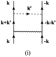
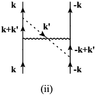
Reading off our effective theory (8), it is of remarkable interest to stress that the attractive Cooper channel interaction (5) can generate three sorts of one-loop diagrams, namely, ZS, $\mathrm{ZS}^{\prime}$ and BCS, which all contribute to the coupling strength $\lambda$ and together play an important role in determining low-energy behaviors [51, 54, 55]. Accordingly, the low-energy properties of 2D SD semimetals, in particular whether the Cooper instability can be ignited, are primarily governed by these one-loop corrections from fermionic attractive interaction together with the chemical potential $\mu$ . In order to examine this within a wide energy regime, we are suggested to derive energy-dependent evolutions of interaction parameters and investigate the low-energy behaviors by virtue of unbiased renormalization group approach, which can treat all potential facets on the same footing and thus capture the mutual effects among all interaction parameters. In this work, we concentrate on one-loop corrections, which are related to Feynman diagrams provided in Figs. 1-4 respectively stemming from Cooper-pairing (Figs. 1, 3) and fermion-impurity interaction (Figs. 1, 2, 4).

III Renormalization-group analysis at clean limit

In this section, we only concentrate on the clean-limit case, namely neglecting $S_{\mathcal{I}}$ in Eq. (8), and leave the analysis in presence of impurity in Sec. V. To be specific, we complete the one-loop RG analysis of effective theory (8) to construct the coupled running equations of all correlated parameters upon lowering the energy scales via adopting the momentum-shell RG method [52, 53, 51]. Along with the standard steps of this RG framework, one integrates out the fast modes of fermionic fields characterized by the momentum shell $b\Lambda<k<\Lambda$ with the variable parameter $b=e^{-l}<1$ and a running energy scale $l$ , then incorporates these fast-mode contributions to the slow modes, and finally rescales the slow modes to new “fast modes” [104, 105, 106, 107, 108, 109, 110, 111, 79, 96, 103]. After performing all these procedures, the coupled flow RG equations of interaction parameters can be derived via comparing new “fast modes” with old “fast modes” in the effective theory.

These coupled flow equations of all interaction parameters are generally pivotal to determine the low-energy physical behaviors. Before moving further, we need to derive the RG rescaling transformations of fields and momenta, which connect two continuous steps of RG processes. In accordance with the spirit of the momentum-shell RG, the non-interacting parts $(-i\omega+\alpha k^{2}_{x}\sigma_{1}+vk_{y}\sigma_{2})$ can be conventionally selected as a starting fixed point, which is invariant during the RG transformations. Under these respects, the RG re-scaling transformations can be extracted as [51, 104, 79],

$\displaystyle k_{x}$	$\displaystyle=$	$\displaystyle k^{\prime}_{x}e^{-\frac{1}{2}l},$	(9)
$\displaystyle k_{y}$	$\displaystyle=$	$\displaystyle k^{\prime}_{y}e^{-l},$	(10)
$\displaystyle\omega$	$\displaystyle=$	$\displaystyle\omega^{\prime}e^{-l},$	(11)
$\displaystyle\Psi(i\omega,\mathbf{k})$	$\displaystyle=$	$\displaystyle\Psi^{\prime}(i\omega^{\prime},\mathbf{k}^{\prime})e^{\frac{1}{2}\int^{l}_{0}dl\left(\frac{7}{2}-\eta\right)},$	(12)

where the parameter $\eta$ is closely linked to the higher-level corrections due to the fermioinc interactions, which characterizes the potentially anomalous dimension of fermionc spinor. It is worth pointing out that these re-scalings can be understood as the bridge between the “old” and “new” fast modes of the effective theory, which would play a vital role in building the coupled RG evolutions of all related interaction parameters.

At this stage, we consequently can concentrate on our RG analyses. As delineated in Eq. (8), there are in all four parameters that we need to care about, namely $\alpha$ , $v$ , $\mu$ , and $\lambda$ . To proceed, we begin with the tree-level case at which we turn off the higher-order corrections. After considering the re-scalings from Eq. (9)-Eq. (12), one can straightforwardly find the evolutions as follows

	$\displaystyle\frac{d\mu}{dl}$	$\displaystyle=$	$\displaystyle\mu,$		(13)
	$\displaystyle\frac{d\lambda}{dl}$	$\displaystyle=$	$\displaystyle-\lambda,$		(14)

and the parameters $d\alpha/dl=dv/dl=0$ . Under this situation, the interaction parameters are evolving independently with decreasing the energy scale. As a result, the correlated low-energy physical behaviors of 2D SD systems cannot be extracted and displayed. In particular, the Cooper instability is directly forbidden by the RG equation of coupling $\lambda$ (14).

In order to capture more physical information and pin down the fate of attractive interaction $\lambda$ in the low-energy regime, we are forced to study the one-loop corrections to the fermionic propagator and strength of fermionic interaction owing to the attractive fermionic interaction. Before going further, we measure the momenta and energy with the cutoff $\Lambda_{0}$ , which is associated with the lattice constant, namely $k\rightarrow k/\Lambda_{0}$ and $\omega\rightarrow\omega/\Lambda_{0}$ [51, 104, 107, 79]. According to one-loop corrections as depicted in Fig. 1 to fermionic propagator, there exists no anomalous fermionic dimension, namely, $\eta=0$ .

In addition, we turn to the one-loop corrections to interaction parameter $\lambda$ , which contain three distinct types of subchannels, namely ZS, $\mathrm{ZS}^{\prime}$ , and BCS subchannels [51] as delineated in Fig. 3. Although both ZS and $\mathrm{ZS}^{\prime}$ diagrams own a finite transfer momentum $\mathbf{Q}=\mathbf{q}-\mathbf{k}$ and $\mathbf{Q}^{\prime}=-\mathbf{q}-\mathbf{k}$ , it is of particular interest for Cooper interaction to point out that $|\mathbf{Q}|\ll|\mathbf{Q}^{\prime}|$ once two external momenta $\mathbf{q}$ and $\mathbf{k}$ possess the same sign (or $|\mathbf{Q}^{\prime}|\ll|\mathbf{Q}|$ if they own opposite signs). For simplicity, we can approximately let $\mathbf{Q}=0$ and take a finite value of $\mathbf{Q}^{\prime}$ or vice versa [51, 78]. Within this work, we also adopt this approximation to simplify our analyses. To be specific, we assume $\mathbf{Q}=0$ and $\mathbf{Q}^{\prime}$ acquires a finite value, which is characterized by two parameters $Q$ and $\varphi$ to measure its strength and direction, respectively. Carrying out several tedious but straightforward calculations gives rise to the following corrections,

$\displaystyle\delta\lambda_{\mathrm{ZS}}\!$	$\displaystyle=$	$\displaystyle\!\frac{\lambda^{2}l(8\mathcal{D}_{1}-4\mu^{2}\mathcal{D}_{0})}{4\pi^{2}},$	(15)
$\displaystyle\delta\lambda_{\mathrm{ZS^{\prime}}}\!$	$\displaystyle=$	$\displaystyle\!\frac{\lambda^{2}l\left[8(\mathcal{D}_{2}-\mathcal{D}_{1}-\sum^{5}_{i=3}\mathcal{D}_{i})+4\mu^{2}\mathcal{D}_{0}\right]}{4\pi^{2}},$	(16)
$\displaystyle\delta\lambda_{\mathrm{BCS}}\!$	$\displaystyle=$	$\displaystyle\!\frac{2\lambda^{2}l\mu^{2}\mathcal{D}_{0}}{4\pi^{2}},$	(17)

where the related coefficients $\mathcal{D}_{i}$ with $i=0$ to $5$ are designated in Eqs. (57)-(60). We hereby emphasize the one-loop corrections at $\mu=0$ can be calculated analogously, which will be studied in details in Sec. IV.1. Based on these one-loop corrections, we derive the coupled RG evolutions at $\mu\neq 0$ :

	$\displaystyle\frac{d\mu}{dl}\!\!$	$\displaystyle=$	$\displaystyle\!\!\!\mu,$		(18)
	$\displaystyle\frac{d\lambda}{dl}\!\!$	$\displaystyle=$	$\displaystyle\!\!\!\left[-1-\frac{\lambda\left(4\mathcal{D}_{2}-4\sum^{5}_{i=3}\mathcal{D}_{i}+\mu^{2}\mathcal{D}_{0}\right)}{4\pi^{2}}\right]\!\!\lambda,$		(19)

where the interaction parameters $d\alpha/dl=dv/dl=0$ .

Before moving further, we now would like to present brief remarks on these coupled RG evolutions of interaction parameters. At first, one-loop RG evolution (19) is qualitatively distinct from their tree-level counterpart (14), namely an additional term is generated no matter $\mu=0$ or $\mu\neq 0$ , which may totally change its low-energy behaviors. This implies that these couplings are not independent and hence their low-energy fates are intimately associated with each other. Accordingly, the low-energy behaviors, compared to their tree-level situations, may be revised or even qualitatively changed. In particular, the fate of parameter $\lambda$ may be changed and Cooper instability may be triggered under certain circumstance. In addition, the coupled RG running equations are of remarkable distinction between zero and a finite chemical potential as the values of DOS at the Dirac point are qualitatively different. One therefore can expect the distinct fates of the interaction coupling $\lambda$ between these two cases, which may correspond to some phase transition. Moreover, what about the behaviors of physical quantities while the system undergoes a potentially tuned phase transition? Whether the Cooper instability can be generated? In the impending sections, we are going to study and response to these questions.

IV Cooper instability and $\mu$ -tuned phase transition at clean limit

Within this section, we endeavor to investigate the effects of attractive Cooper-pairing interaction and chemical potential on the low-energy behaviors of interaction coupling $\lambda$ by virtue of both theoretical and numerical analyses of the one-loop RG evolutions, which are established in Sec. III and intertwine all related interaction parameters together and . Based on these information, we would examine whether the Cooper instability can be triggered at $\mu=0$ and what conditions are required to trigger the Cooper instability for our 2D SD systems. In addition, since the DOS at Fermi surface (Dirac point) is qualitatively distinct between $\mu=0$ and $\mu\neq 0$ in 2D SD semimetals [1, 34, 25], one may expect a chemical potential-tuned ( $\mu$ -tuned) phase transition, which is conventionally accompanied by unique behaviors in the vicinity of the critical point, for instance, the Cooper instability attesting to its sensitivity to the Dirac point.

IV.1 Cooper instability at $\mu=0$

At the outset, we recall the tree-level results on the interaction coupling $\lambda$ depicted in Eq. (14). In particular, we highlight that it flows independently with parameters $\alpha$ and $v$ upon decreasing the energy scales. Accordingly, once the parameter $\lambda$ is taken an initially attractive value, we can easily find that Cooper instability cannot be activated as $\lambda$ goes towards zero upon lowering energy scale. This indicates that the Cooper theorem is manifestly violated. One may mainly ascribe this unusual feature to the vanish of density of states at the Dirac point [34, 32, 25].

In the spirit of RG theory, the higher-order corrections are required to be involved to judge the stability of tree-level conclusion and further pin down the fate of $\lambda$ at the low-energy region. To this end, we calculate the one-loop contributions to the parameter $\lambda$ , which are consist of three subtypes, i.e., ZS, $\mathrm{ZS}^{\prime}$ and BCS channels [51] as listed in Eqs. (15)-(17). To be concrete, These one-loop corrections at $\mu=0$ are derived as

$\displaystyle\delta\lambda_{\mathrm{ZS}}$	$\displaystyle=$	$\displaystyle\frac{8\lambda^{2}l\mathcal{D}_{1}}{4\pi^{2}},$	(20)
$\displaystyle\delta\lambda_{\mathrm{ZS^{\prime}}}$	$\displaystyle=$	$\displaystyle\frac{8\lambda^{2}l\left(\mathcal{D}_{2}-\mathcal{D}_{1}-\sum^{5}_{i=3}\mathcal{D}_{i}\right)}{4\pi^{2}},$	(21)
$\displaystyle\delta\lambda_{\mathrm{BCS}}$	$\displaystyle=$	$\displaystyle 0.$	(22)

One needs to bear in mind during the derivations that there are qualitative distinctions between 2D DSM, which possess linear dispersions for both $k_{x}$ and $k_{y}$ directions, and our 2D SD semimetals. Accordingly, the coupled evolutions of interaction parameters are derived as follows,

	$\displaystyle\frac{d\alpha}{dl}$	$\displaystyle=$	$\displaystyle\frac{dv}{dl}=0,$		(23)
	$\displaystyle\frac{d\lambda}{dl}$	$\displaystyle=$	$\displaystyle\left[-1-\frac{\lambda\left(4\mathcal{D}_{2}-4\sum^{5}_{i=3}\mathcal{D}_{i}\right)}{4\pi^{2}}\right]\lambda.$		(24)

Before moving further, we again stress that both one-loop corrections (20)-(22) and RG equations (23)-(24) are calculated and derived separately.

Learning from Eqs. (20)-(22), it is of particular interest to point out that the BCS subchannel of Cooper-pairing interaction does not contribute any corrections to the interaction coupling $\lambda$ . As a consequence, this subchannel does not participate in the coupled RG evolutions and contribute to potential emergence of Cooper instability. This exhibits a sharp contrast to the situation of 2D DSM materials, at which the BCS subchannel plays a central role in igniting the Cooper instability (also dubbed as the BCS instability owing to its leading contribution) if the initial value of Cooper coupling exceeds certain critical value [54, 78]. We would like to pause hereby and remark on the underline logic that is responsible for their differences. In brief, the cardinal facet is ascribed to the distinct dispersions of low-energy fermionic excitations. In the BCS subchannel, the transfer momentum is zero, namely $\mathbf{Q}=0$ and thus its correction is proportional to $\mathrm{Tr}(\sigma_{2}G(i\omega,\mathbf{k})\sigma_{2}G(i\omega,-\mathbf{k}))$ . With respect to the 2D DSM systems, their dispersions are linear for both $k_{x}$ and $k_{y}$ directions, i.e., $G^{-1}(i\omega,\mathbf{k})\sim(-i\omega+c_{1}k_{x}\sigma_{1}+c_{2}k_{y}\sigma_{2})$ with $c_{1}$ and $c_{2}$ being some constants. As a result, corrections from $k_{x}$ and $k_{y}$ parts are mutually neutralized each other and thus the $\omega$ term gains a finite contribution. Compared manifestly to the 2D DSM’s dispersion, our 2D SD semimetals possess anisotropic excitations along $k_{x}$ and $k_{y}$ orientations, namely $G^{-1}_{\mathrm{SD}}(i\omega,\mathbf{k})\sim(-i\omega+c_{1}k^{2}_{x}\sigma_{1}+c_{2}k_{y}\sigma_{2})$ . This consequently renders that $k_{x}$ and $k_{y}$ corrections support each other and finally their summation counteracts with the correction from $(-i\omega)$ part. It therefore leads to the vanish of BCS subchannel at $\mu=0$ .

We next turn to the contributions from the ZS and $\mathrm{ZS}^{\prime}$ subchannels. Specifically, we find that both ZS and $\mathrm{ZS}^{\prime}$ diagrams can contribute to the RG running of parameter $\lambda$ once the transfer momentum $\mathbf{Q}$ is nonzero. An exception is that the summation of ZS and $\mathrm{ZS}^{\prime}$ subchannels can be neutralized exactly in the case of $\mathbf{Q}=0$ . According to the information above, we obtain that the coupling $\lambda$ ’s flow equation (24) at $\mu=0$ only collects the contributions from ZS and $\mathrm{ZS}^{\prime}$ diagrams. This indicates that, at zero chemical potential, the energy-dependent evolution of coupling $\lambda$ primarily hinges upon the ZS plus $\mathrm{ZS}^{\prime}$ not BCS subchannels, to be more specifically, the transfer momenta $\mathbf{Q}$ . As a consequence, it is tempting to ask whether the one-loop corrections from ZS and $\mathrm{ZS}^{\prime}$ diagrams due to the Cooper-pairing interaction can produce the Cooper instability and how it is related to the transfer momentum $\mathbf{Q}$ .

To proceed, we initially endeavor to study $\lambda$ ’s evolution (24) analytically. One can infer the critical strength of starting value of $\lambda$ via assuming Eq. (24)’s left hand side equals to zero, namely

\displaystyle\lambda_{c}(0)

\displaystyle=

\displaystyle\frac{\pi^{2}}{\left(\sum^{5}_{i=3}\mathcal{D}_{i}-\mathcal{D}_{2}\right)}.

(25)

This forthrightly singles out that the Cooper instability can be formally ignited once the initial strength $|\lambda(0)|$ exceeds the critical value $|\lambda_{c}(0)|$ while the parameters $\mathcal{D}_{i}$ are regarded as constants. However, it is of particular interest to point out that $\lim_{\mathbf{Q}\rightarrow 0}|\lambda_{c}(0)|\rightarrow\infty$ attesting to the defined functions $\mathcal{D}_{i}(\mathbf{Q}=0)\rightarrow 0$ with $i=2$ to $5$ . Therefore, the Cooper instability is unable to be generated and this is consistent with our previous analyses that the transfer momentum $\mathbf{Q}$ plays a crucial role. In order to explicitly show the tendencies of parameter $\lambda$ upon decreasing the energy scale, we are suggested to calculate the RG equation numerically by adopting several representatively beginning values of correlated parameters. Particularly, as the low-energy fate of $\lambda$ is closely linked to the momentum $\mathbf{Q}$ , we introduce two variables, i.e., $Q$ and $\varphi$ , to denote its strength and direction, respectively. As the parameter $Q$ carries the property of momentum, we also measure it with the cutoff $\Lambda_{0}$ in the following numerical calculations. The corresponding results are gathered in Fig. 5 and Fig. 6. We next address them in details.

At first, we make our focus on two special angles, at which the $(\sum^{5}_{i=3}\mathcal{D}_{i}-\mathcal{D}_{2})=0$ (independent of the value of $Q$ ), namely $\varphi_{1}=\pi/2$ and $\varphi_{2}=3\pi/2$ . Hence, they are equivalent to the case of $Q=0$ and directly reduce to the tree level case (the lines are overlapped, namely independent of $Q$ ). Therefore, the Cooper instability cannot be triggered as depicted in Fig. 5(a) (the results for $\varphi_{2}=3\pi/2$ are the same to $\varphi_{1}=\pi/2$ ’s and thus are not shown in the figure). For convenient reference, we hereby name these two special points as $\varphi\in\mathrm{Zone-O}$ .

Subsequently, all other angles cluster into two groups. We call them Zone-I and Zone-II determined by $\alpha$ , $v$ , and $Q$ , at which $(\sum^{5}_{i=3}\mathcal{D}_{i}-\mathcal{D}_{2})$ would be positive and negative respectively, namely

	$\displaystyle\varphi\in\mathrm{Zone-I}:\,\,\,\left(\sum^{5}_{i=3}\mathcal{D}_{i}-\mathcal{D}_{2}\right)>0,$		(26)
	$\displaystyle\varphi\in\mathrm{Zone-II}:\,\,\,\left(\sum^{5}_{i=3}\mathcal{D}_{i}-\mathcal{D}_{2}\right)<0.$		(27)

We then consider them one by one. At Zone-I, we find that the Cooper instability cannot be activated although it is sensitive to the transfer momentum $\mathbf{Q}$ upon increasing $Q$ and $|\lambda_{0}|$ as shown in Fig. 5(b) for a representative angle $\varphi=\pi/3$ . To be concrete, this can be understood strictly. Compared to the tree-level flow, it behaviors as $d\lambda/dl=-(1+C)\lambda$ with the constant $C>0$ at Zone-I, which therefore cannot produce the Cooper instability. In a sharp contrast, the Cooper instability can be generated at Zone-II with the same initial conditions of Fig. 5. Choosing two representative angles $\varphi=0$ and $\varphi=\pi/3$ at Zone-II and carrying out the numerical evaluations give rise to the results delineated in Fig. 6. Studying from Fig. 6, we find the Cooper instability can be manifestly triggered by virtue of increasing $Q$ at a fixed $\lambda(0)$ delineated in Fig. 6(a) or enlarging $|\lambda(0)|$ at a fixed $Q$ illuminated in Fig. 6(b) for two representative Zone-II angles $\varphi=5\pi/6$ and $\varphi=\pi$ , respectively. It is worth pointing out that the basic results of Fig. 6 are insensitive to the initial values of parameters, for instance $\alpha$ and $v$ (we assume that they are small compared to the cutoff), which would only determine the critical energy scale at which the Cooper instability sets in. All these numerical results are in line with our above analytical analyses.

Before going further, we hereby stop to present several discussions on the ranges of both $\mathrm{Zone-I}$ and $\mathrm{Zone-II}$ , which are closely associated with the sign of $\left(\sum^{5}_{i=3}\mathcal{D}_{i}-\mathcal{D}_{2}\right)$ . To proceed, we nominate the $\mathcal{F}(\varphi)$ as

	$\displaystyle\mathcal{F}(\varphi)$	$\displaystyle\equiv$	$\displaystyle\sum^{5}_{i=3}\mathcal{D}_{i}-\mathcal{D}_{2}=(\mathcal{M}\cos^{3}\varphi+\mathcal{N}\cos^{2}\varphi$		(28)
			$\displaystyle+\mathcal{O}\cos\varphi+\mathcal{P})\cos\varphi.$		(28)

Then the slope of function $\mathcal{F}(\varphi)$ with respect to $\varphi$ can be derived as

	$\displaystyle\mathcal{F}^{\prime}(\varphi)$	$\displaystyle=$	$\displaystyle\frac{d\mathcal{F}(\varphi)}{d\varphi}=-(4\mathcal{M}\cos^{3}\varphi+3\mathcal{N}\cos^{2}\varphi$		(29)
			$\displaystyle+2\mathcal{O}\cos\varphi+\mathcal{P})\sin\varphi,$		(29)

where the coefficients $\mathcal{M}$ , $\mathcal{N}$ , $\mathcal{O}$ , and $\mathcal{P}$ are defined in Eqs. (61)-(64).

To facilitate our discussions, we then divide the full region of $\varphi$ into Zone-O plus four subregions, namely $\mathrm{Region-A}\in[0,\frac{\pi}{2})$ , $\mathrm{Region-B}\in(\frac{\pi}{2},\pi)$ , $\mathrm{Region-C}\in(\pi,\frac{3\pi}{2})$ , and $\mathrm{Region-D}\in(\frac{3\pi}{2},2\pi]$ . For $\varphi\in\mathrm{Region-A}$ , we can straightforwardly get $\mathcal{F}(\varphi=0)>0$ and $\lim_{\varphi\rightarrow\frac{\pi}{2}}\mathcal{F}(\varphi)=0$ . In addition, in order to make the two-dimensional semi-Dirac systems stable, the distinction between the values of $\alpha$ and $v$ is very small (if we assume $\alpha\gg v$ or $v\gg\alpha$ , the dispersion of our system would directly reduce to the full parabolic or linear situations). Moveover, the value of transfer momenta $|\mathbf{Q}|$ is much smaller than other parameters. Gather all these factors together, we can obtain that the slope of function $\mathcal{F}(\varphi)$ satisfies $\mathcal{F}^{\prime}(\varphi)<0$ . Therefore, $\mathcal{F}(\varphi)$ monotonically decreases and gradually evolves from a positive value towards zero, namely $\mathrm{Region-A}\in\mathrm{Zone-I}$ . Similarly, one can obtain $\mathrm{Region-D}$ also belongs to $\mathrm{Zone-I}$ . On the contrary, one can get $\lim_{\varphi\rightarrow\frac{\pi}{2}}\mathcal{F}(\varphi)=0$ and $\mathcal{F}^{\prime}(\varphi)<0$ for $\varphi\in\mathrm{Region-B}$ . Analogously, for $\varphi\in\mathrm{Region-C}$ , it reads that $\mathcal{F}(\varphi=\pi)<0$ and $\lim_{\varphi\rightarrow\frac{3\pi}{2}}\mathcal{F}(\varphi)=0$ as well as $\mathcal{F}^{\prime}(\varphi)>0$ . Consequently, these analyses can tell us that $\mathcal{F}(\varphi)<0$ for $\mathrm{Region-B}$ and $\mathrm{Region-C}$ , namely, $\mathrm{Zone-II}$ consisting of both $\mathrm{Region-B}$ and $\mathrm{Region-C}$ . Before closing the discussions, we stress again that the sign of function $\mathcal{F}$ strongly depends upon $\varphi$ although its value is slightly sensitive to $Q$ . Based on both analytical and numerical analysis above, one can find that the overall structures and signs of $\mathcal{F}(\varphi)$ are very insensitive to $Q$ but are even solely determined by $\varphi$ as long as $Q$ is small (this can be always satisfied as $Q$ is a transfer momentum) as manifestly shown in Fig. 7 and Fig. 8.

In order to verify our analytical discussions, we perform the numerical calculations via taking several representative values of $Q$ , $v$ , and $\alpha$ and obtain the the results shown in Fig. 7, which are well consistent with above analyses. Based on above discussions, we can draw a conclusion that the Cooper instability can be generated while $\varphi$ is restricted to $\mathrm{Zone-II}$ with a nonzero value of $|\mathbf{Q}|$ . Additionally, we would like to stress that $\mathrm{Zone-II}$ including both $\mathrm{Region-B}$ and $\mathrm{Region-C}$ is not small but nearly takes half of full directions (regions) ( $\frac{\pi}{2}$ and $\frac{3\pi}{2}$ do not belong to $\mathrm{Zone-II}$ ) as schematically shown in Fig. 8. Before closing this section, let us hereby address some comments on possibly physical pictures for the ranges of $\mathrm{Zone-I}$ and $\mathrm{Zone-II}$ . Specifically, if we consider the regions $\varphi\in(\frac{\pi}{2},\frac{3\pi}{2})$ and $\varphi\in[0,\frac{\pi}{2}]\mathrm{U}[\frac{3\pi}{2},2\pi]$ as the so called “forward-alike scattering” and “back-alike scattering”, respectively, one may realize that above analysis implies that only the“forward-alike scattering” associated with the transfer momentum $\mathbf{Q}_{\varphi_{\mathrm{II}}}$ can contribute to the Cooper instability as schematically shown in Fig. 8. On the contrary, the “back-alike scattering” can not provide useful corrections to Cooper instability. This picture should be also physically reasonable.

To recapitulate, we have examined how the Cooper-pairing interaction influences the low-energy states of 2D SD materials at $\mu=0$ , in particular the possibility of Cooper instability. Table 1 and Fig. 8 summarize our main results for both $\mu=0$ and $\mu\neq 0$ . In next subsection, we are going to investigate the situation in the presence of a finite chemical potential.

Table 1: Collections of basic conclusions for Cooper instability (CI) due to one-loop corrections of Cooper-pairing interaction for both zero and a finite chemical potential. The terminology “CI always generated” means that the CI can be triggered at an arbitrarily weak Cooper-pairing coupling strength

\lambda

. The “Zone-O” corresponds to

\varphi=\frac{\pi}{2},\frac{3\pi}{2}

and “Zone-I” and “Zone-II” are designated in Eq. (26) and Eq. (27), respectively.

$\mu=0$ , $Q=0$ or $\varphi\in\mathrm{Zone-O}$ No CI $\mu=0$ , $Q\neq 0$ , $\varphi\in\mathrm{Zone-I}$ No CI $\mu=0$ , $Q\neq 0$ , $\varphi\in\mathrm{Zone-II}$ CI triggered at $|\lambda(0)|>|\lambda_{c}(0)|$ $\mu\neq 0$ CI always generated

IV.2 $\mu$ -tuned phase transition

As addressed at the beginning of this section, the $\mu$ -tuned phase transition is expected in that the DOS at Fermi surface for zero chemical potential is qualitatively distinct from a finite- $\mu$ situation’s [1, 34, 25]. Under such circumstance, one naturally concerns the question whether and how this phase transition is linked to the Cooper instability.

To response these, paralleling the analysis for $\mu=0$ part, we can initially derive the formal $\lambda_{c}(0)$ with hypothesizing all other parameters to be constants by virtue of referring to Eq. (19),

\displaystyle\lambda_{c}(0)

\displaystyle=

\displaystyle\frac{4\pi^{2}}{4\left(\sum^{5}_{i=3}\mathcal{D}_{i}-\mathcal{D}_{2}\right)-\mu^{2}\mathcal{D}_{0}}.

(30)

Before going further, we recall pieces of useful information obtained in Sec. IV.1: $D_{i}(Q\rightarrow 0)=0$ or $D_{i}(\varphi=\pi/2)=D_{i}(\varphi=3\pi/2)=0$ with $i=2$ to $5$ and the sign of $(\sum^{5}_{i=3}\mathcal{D}_{i}-\mathcal{D}_{2})$ is positive or negative respectively corresponding to $\varphi\in\mathrm{Zone-I}$ and $\varphi\in\mathrm{Zone-II}$ . With respect to this information, this critical coupling, at the first sight, is very analogous to the case with $\mu=0$ , $Q\neq 0$ , and $\varphi\in\mathrm{Zone-II}$ , indicating the Cooper instability being produced at $|\lambda(0)|>|\lambda_{c}(0)|$ as listed in Table 1. However, we would like to emphasize that these two circumstances are qualitatively distinct. In the former, the coupling $\lambda_{c}(0)$ are constants that determined by the values of $\alpha$ , $v$ , and $Q$ . Conversely, the $\lambda_{c}(0)$ for the latter evolves towards zero in that the chemical potential $\mu$ is a relevant quantity by means of RG term as characterized in Eq. (18), which climbs up upon lowering the energy scales. As a result, it implies any weak attractive interaction can ignite the Cooper pairing once a finite $\mu$ is introduced, namely the Cooper theorem [50]. This result is well consistent with the mean-field analysis of 2D Dirac semimetals [112, 113], which can be generally understood as follows. As a finite $\mu$ changes the Dirac point and the DOS is nonzero at Fermi surface, this causes the BCS diagram also contributes to the parameter $\lambda$ , which becomes the very dominant subchannel. To explicitly display the process, the numerical evolutions of $\lambda$ for the presence of a representative $\mu$ are provided in Fig. 9(a) at $D_{i}=0$ . To proceed, an intriguing question is raised whether the outcome above is sufficiently robust against a finite $Q$ at Zone-II, namely the fate of competition between $4(\sum^{5}_{i=3}\mathcal{D}_{i}-\mathcal{D}_{2})$ and $\mu$ . In order to response this, we would like to select out several representatively starting values of parameters at Zone-II, which are the same to their counterparts in Fig. 6. Additionally, we bring out a very small starting value of $\mu$ , for instance $\mu=10^{-5}$ and numerically evaluate the running evolutions of $\mu$ and $\lambda$ (18)-(19), leading to the corresponding results in Fig. 9(b). To reiterate, we stress that the basic results of Fig. 9 are insensitive to the concrete beginning values of $\mu$ .

Reading off the information in Fig. 9 and gathering all these analyses and discussions together, we therefore come to a conclusion that a finite $\mu$ indeed play an essential role in triggering the Cooper instability and a $\mu$ -tuned phase transition associated with the Cooper instability can be expected [49, 114].

V Cooper instability influenced by the impurity scattering at $\mu=0$

It is well known that the impurities are present in nearly all fermionic systems, whose effects on the low-energy behaviors of physical quantities are widely investigated [80, 81, 83, 84, 85, 86, 87, Nandkishore2013PRB, Potirniche2014PRB, 88, 82, 89, 90, 91, 92, 93, 94, 115, 95]. Generally, impurity scatterings can induce the damping rate of fermions, which can both promote fermionic excitations with shortening their lifetimes to be harmful for the superconductivity and enhance the DOS of fermionic systems to be helpful for the superconductivity. Accordingly, it is worth asking how the impurity influences the Cooper instability under the competition between these two adverse sorts of contributions.

As addressed in previous section, we attentively investigate the emergence of Cooper instability for the presence of both zero and a finite chemical potential at clean limit. One of most significant points in this situation is that a finite chemical potential $\mu$ plays a central role in low-energy regime and can always induce the Cooper instability. Therefore, we here focus on the situation at $\mu=0$ and briefly discuss the effects of impurities on the formation of Cooper instability.

Based on one-loop corrections provided in Appendix B, we arrive at the updated RG equations of interaction parameters for the presence of multi types of impurities,

$\displaystyle\frac{d\alpha}{dl}$	$\displaystyle=$	$\displaystyle\frac{[-(\Delta_{C}+\Delta_{G_{1}})\mathcal{E}_{0}]\alpha}{4\pi^{2}},$	(31)
$\displaystyle\frac{dv}{dl}$	$\displaystyle=$	$\displaystyle\frac{[-(\Delta_{C}+\Delta_{M})\mathcal{E}_{0}]v}{4\pi^{2}},$	(32)
$\displaystyle\frac{d\Delta_{C}}{dl}$	$\displaystyle=$	$\displaystyle\frac{\Bigl[\sum_{I\neq C}\Delta_{I}\mathcal{E}_{1}-\Delta_{C}\mathcal{E}_{2}\Bigr]\Delta_{C}}{4\pi^{2}},$	(33)
$\displaystyle\frac{d\Delta_{G_{1}}}{dl}$	$\displaystyle=$	$\displaystyle\frac{1}{4\pi^{2}}\Bigl[-(\Delta_{G_{3}}+\Delta_{M})\mathcal{E}_{1}-\Delta_{G_{1}}\mathcal{E}_{2}$	(34)
		$\displaystyle+\Delta_{C}(\mathcal{E}_{1}-2\mathcal{E}_{2})\Bigr]\Delta_{G_{1}},$	(34)
$\displaystyle\frac{d\Delta_{G_{3}}}{dl}$	$\displaystyle=$	$\displaystyle\frac{1}{4\pi^{2}}\Bigl[(\Delta_{G_{1}}+\Delta_{M})\mathcal{E}_{1}-\Delta_{G_{3}}\mathcal{E}_{2}$	(35)
		$\displaystyle+\Delta_{C}(\mathcal{E}_{1}-2\mathcal{E}_{0})\Bigr]\Delta_{G_{3}},$	(35)
$\displaystyle\frac{d\Delta_{M}}{dl}$	$\displaystyle=$	$\displaystyle\frac{1}{4\pi^{2}}\Bigl[(\Delta_{G_{1}}+\Delta_{G_{3}})(\mathcal{E}_{1}-2\mathcal{E}_{2})-\Delta_{C}\mathcal{E}_{1}$	(36)
		$\displaystyle-\Delta_{M}\mathcal{E}_{2}+4\lambda(\mathcal{E}_{1}-\mathcal{E}_{2})\Bigr]\Delta_{M},$	(36)

combined together with

\displaystyle\frac{d\lambda}{dl}\!=\!\left[\!-1-\frac{\lambda\left(4\mathcal{D}_{2}-4\sum^{5}_{i=3}\mathcal{D}_{i}\right)}{4\pi^{2}}-\frac{\sum_{I}\Delta_{I}\mathcal{E}_{2}}{4\pi^{2}}\!\right]\!\!\lambda.

(37)

where the parameters again $C$ , $G_{1,3}$ , and $M$ denote the random chemical potential, random gauge potential and random mass, respectively.

Subsequently, we examine the influence of impurity on the Cooper instability. At first, we can derive the formally critical value of $\lambda$ via paralleling the analyses in Sec. IV.1. Reading off Eq. (37), the $\lambda_{c}(0)$ can be extracted as,

\displaystyle\lambda_{c}(0)

\displaystyle=

\displaystyle\frac{\pi^{2}\left(1+\frac{\sum_{I}\Delta_{I}\mathcal{E}_{2}}{4\pi^{2}}\right)}{\left(\sum^{5}_{i=3}\mathcal{D}_{i}-\mathcal{D}_{2}\right)}.

(38)

In comparison with its clean-limit and $\mu=0$ counterpart (25), one can directly find that the critical strength $\lambda_{c}(0)$ is manifestly increased due to the impurity scatterings as long as the parameters $\alpha$ and $v$ are constants. However, we need to emphasize that Eqs. (31)-(37) unambiguously exhibit that all parameters are not independent but intimately coupled with each others. With this respect, it is necessary to perform the numerical calculation along these coupled flow equations to explicitly show the fate of parameter $\lambda$ at low-energy scales.

As it is of particular interest to examine the effects of impurity scatterings on the Cooper instability, we hereby only focus on the situations at which the Cooper instability can be ignited potentially at the clean limit, namely $\varphi\in\mathrm{Zone-II}$ . For completeness, the presence of single and multi sorts of impurities will be both investigated. At the outset, we assume only one type of impurity exists in the system. To proceed, we derive the reduced RG equations for the presence of random chemical potential via assuming $\Delta_{I\neq C}=0$ in Eqs. (31)-(37),

$\displaystyle\frac{d\alpha}{dl}$	$\displaystyle=$	$\displaystyle\frac{-\Delta_{C}\mathcal{E}_{0}}{4\pi^{2}}\alpha,$	(39)
$\displaystyle\frac{dv}{dl}$	$\displaystyle=$	$\displaystyle\frac{-\Delta_{C}\mathcal{E}_{0}}{4\pi^{2}}v,$	(40)
$\displaystyle\frac{d\Delta_{C}}{dl}$	$\displaystyle=$	$\displaystyle\frac{-\Delta^{2}_{C}\mathcal{E}_{2}}{4\pi^{2}},$	(41)
$\displaystyle\frac{d\lambda}{dl}$	$\displaystyle=$	$\displaystyle\left(-1-\lambda_{\mathcal{D}}-\frac{\Delta_{C}\mathcal{E}_{2}}{4\pi^{2}}\right)\lambda,$	(42)

with designating $\lambda_{\mathcal{D}}\equiv\lambda\left(\mathcal{D}_{2}-\sum^{5}_{i=3}\mathcal{D}_{i}\right)/(\pi^{2})$ .

One can obviously read that the random chemical potential is decreased progressively upon lowering the energy scales, namely an irrelevant quantity in the RG terminology. This indicates that its effects are gradually weakened as the energy is lowered due to its irrelevant feature. However, the $\lambda$ couples with the strength of impurity as well as the parameters $\alpha$ and $v$ , which also evolve and are associated with the $\mathcal{D}_{i}$ and $\lambda_{\mathcal{D}}$ . This implies that the value of $\lambda_{c}(0)$ (38) can either be increased or lowered caused by the energy-dependent evolutions of $\mathcal{D}_{i}$ . In order to judge this, we therefore need to perform the numerical analyses of these reduced evolutions of Eqs. (39)-(42). To straightforwardly compared with the clean-limit case, we start with the same starting conditions of Fig. 6, which contains the main results at $\mu=0$ . To be specific, we assign two typical values to $Q$ and $\varphi$ , for instance $Q=10^{-3}$ and $\varphi=\pi$ as utilized in Fig. 6(b). After performing numerical calculations of Eqs. (39)-(42), we find that the Cooper instability is fairly insensitive to this sort of impurity, which only results in the increase of the critical energy scale (i.e., decrease of $l_{c}$ ) where the instability is ignited as designated in Fig. 10. In other words, attesting to the evolutions of parameters $\alpha$ and $v$ , the single presence of random chemical potential is slightly favorable to the Cooper instability although the impurity is an irrelevant quantity. This is of particular distinction from the Dirac semimetals [54, 55, 78].

In addition, for the presence of only random gauge potential or random mass, the coupled evolutions reduce to

$\displaystyle\frac{d\alpha}{dl}$	$\displaystyle=$	$\displaystyle\frac{-\Delta_{G_{1}}\mathcal{E}_{0}}{4\pi^{2}}\alpha,\,\,\frac{dv}{dl}=0,$	(43)
$\displaystyle\frac{d\Delta_{G_{1}}}{dl}$	$\displaystyle=$	$\displaystyle\frac{(-\Delta_{G_{3}}\mathcal{E}_{1}-\Delta_{G_{1}}\mathcal{E}_{2})}{4\pi^{2}}\Delta_{G_{1}},$	(44)
$\displaystyle\frac{d\Delta_{G_{3}}}{dl}$	$\displaystyle=$	$\displaystyle\frac{(\Delta_{G_{1}}\mathcal{E}_{1}-\Delta_{G_{3}}\mathcal{E}_{2}]}{4\pi^{2}}\Delta_{G_{3}},$	(45)
$\displaystyle\frac{d\lambda}{dl}$	$\displaystyle=$	$\displaystyle\left[-1-\lambda_{\mathcal{D}}-\frac{(\Delta_{G_{1}}+\Delta_{G_{3}})\mathcal{E}_{2}}{4\pi^{2}}\right]\lambda,$	(46)

$\displaystyle\frac{d\alpha}{dl}$	$\displaystyle=$	$\displaystyle 0,\,\,\frac{dv}{dl}=\frac{-\Delta_{M}\mathcal{E}_{0}}{4\pi^{2}}v,$	(47)
$\displaystyle\frac{d\Delta_{M}}{dl}$	$\displaystyle=$	$\displaystyle\frac{4\lambda(\mathcal{E}_{1}-\mathcal{E}_{2})-\Delta_{M}\mathcal{E}_{2}}{4\pi^{2}}\Delta_{M},$	(48)
$\displaystyle\frac{d\lambda}{dl}$	$\displaystyle=$	$\displaystyle\left(-1-\lambda_{\mathcal{D}}-\frac{\Delta_{M}\mathcal{E}_{2}}{4\pi^{2}}\right)\lambda.$	(49)

To proceed, after paralleling the analyses for the single presence of random chemical potential and carrying out analogous numerical analyses along the Eqs. (43)-(49), we obtain the primary the results for the random gauge potential and random mass as delineated in Fig. 11 and Fig. 12, respectively. To be concrete, we find that the critical energy scales are decreased (i.e., increase of $l_{c}$ ) by the influence of random gauge potential as depicted in Fig. 11. As a result, in distinction to the random chemical potential, the sole presence of random gauge potential is slightly harmful to the Cooper instability. In a sharp contrast, the coupled evolution equations for the sole presence of random mass yield to several unusual features compared to both random chemical potential and random gauge potential as designated in Fig. 12. At first, it is of particular importance to address that the critical value of fermion-fermion strength $|\lambda(l)|$ , as manifestly illustrated in Fig. 13, quickly climbs certain saturate peak and then gradually flows toward zero at the lowest energy limit. In addition, the starting points of saturate lines are shifted to bigger energy scales with the increase of impurity’s initial values. In other words, the fermion-fermion interaction’s strength $|\lambda(l)|$ is no longer divergent. As a consequence, the Cooper instability is switched off by the random mass with an adequately large starting value.

Next, we consider the situation for presence of all three sorts of impurities. Without loss of generality, all these three types of impurities are assumed to own the equally starting strengths. To proceed, paralleling the analogous steps combined with the coupled flow equations (31)-(37) leads to the main results shown in Fig. 13. According to this figure, we find the fate of fermion-fermion strength is similar to the sole presence of random mass. However, it is of particular significance to point out that the saturated values are much higher due to the competition among these three sorts of impurities. Accordingly, distinct types of impurities compete with each other and eventually the random mass becomes dominant. In other words, this indicates that the fermionic excitations promoted by impurities play a more important role than the increase of DOS in 2D SD semimetals. To reiterate, we hereby stress that the competition among distinct sorts of impurities is harmful to the Cooper instability no matter whether any of single types of impurities promotes or hinders the Cooper instability.

In brief, it is well known that there is a long history for the the effect of impurity on the superconductivity [116, 117, 118, 80], which is a complicate problem and attracted a number of studies for both conventional and unconventional superconductors. We admit that our focuses here are only on the qualitative roles of three types of impurities and the studies here are somehow tentative. Despite this, one can expect the results would provide several significant signals and tendencies of these impurities in the low-energy regime.

VI Competition between the impurities and a nonzero chemical potential

Based on the analyses in Sec. IV and Sec. V for 2D SD systems, we address that the Cooper instability is greatly promoted by the chemical potential. Conversely, the presence of impurities is harmful to the Cooper instability. These imply that the low-energy physics of 2D SD materials would be largely dependent upon which of these two facets is dominant. It therefore is interesting to ask whether and how the fate of Cooper instability would be revised or totally changed under the competition between the impurities and a nonzero chemical potential.

In order to investigate their competition and answer above question, we assume that the chemical potential and impurities are present simultaneously. To proceed, we implement the full effective action (8) and evaluate all one-loop corrections of Fig. 1-4 with both nonzero $\mu$ and all three sorts of impurities. After paralleling long but straightforward calculations as provided in Sec. IV and Sec. V, we derive the corresponding energy-dependent evolutions as

$\displaystyle\frac{d\alpha}{dl}\!\!\!\!$	$\displaystyle=$	$\displaystyle\!\!\!\!\frac{[-(\Delta_{C}+\Delta_{G_{1}})\mathcal{E}_{0}]\alpha}{4\pi^{2}},\,\,\,\frac{dv}{dl}\!=\!\frac{[-(\Delta_{C}+\Delta_{M})\mathcal{E}_{0}]v}{4\pi^{2}},\,\,\,\frac{d\Delta_{C}}{dl}\!=\!\frac{\left[\sum_{I\neq C}\Delta_{I}\mathcal{E}_{1}+\Delta_{C}(\mu^{2}\mathcal{E}_{4}-\mathcal{E}_{2})\right]\!\Delta_{C}}{4\pi^{2}},$	(50)
$\displaystyle\frac{d\Delta_{G_{1}}}{dl}\!\!\!\!$	$\displaystyle=$	$\displaystyle\!\!\!\!\frac{\left[\Delta_{C}(\mathcal{E}_{1}-2\mathcal{E}_{2}+\mu\mathcal{E}_{3})-(\Delta_{M}+\Delta_{G_{3}})(\mu\mathcal{E}_{3}+\mathcal{E}_{1})+\Delta_{G_{1}}(\mu\mathcal{E}_{3}-\mu^{2}\mathcal{E}_{4}-\mathcal{E}_{2})\right]\!\Delta_{G_{1}}}{4\pi^{2}},$	(51)
$\displaystyle\frac{d\Delta_{G_{3}}}{dl}\!\!\!\!$	$\displaystyle=$	$\displaystyle\!\!\!\!\frac{\left[(\Delta_{G_{1}}+\Delta_{M})(\mathcal{E}_{1}-\mu^{2}\mathcal{E}_{4})+\Delta_{C}(\mathcal{E}_{1}-2\mathcal{E}_{0}+\mu^{2}\mathcal{E}_{4})-\Delta_{G_{3}}(\mathcal{E}_{2}+2\mu\mathcal{E}_{4})\right]\!\Delta_{G_{3}}}{4\pi^{2}},$	(52)
$\displaystyle\frac{d\Delta_{M}}{dl}\!\!\!\!$	$\displaystyle=$	$\displaystyle\!\!\!\!\frac{\left[(\Delta_{G_{1}}\!+\!\Delta_{G_{3}})(\mathcal{E}_{1}\!-\!2\mathcal{E}_{2}\!-\!\mu^{2}\mathcal{E}_{4}\!-\!2\mu\mathcal{E}_{3})\!-\!\Delta_{C}(\mathcal{E}_{1}\!-\!\mu^{2}\mathcal{E}_{4}\!+\!2\mu\mathcal{E}_{3})\!-\!\Delta_{M}(\mathcal{E}_{2}\!+\!2\mu\mathcal{E}_{3})\!+\!4\lambda(\mathcal{E}_{1}\!-\!\mathcal{E}_{2}\!-\!\mu^{2}\mathcal{E}_{4})\right]\!\Delta_{M}}{4\pi^{2}},$	(53)
$\displaystyle\frac{d\lambda}{dl}\!\!\!\!$	$\displaystyle=$	$\displaystyle\!\!\!\!\frac{\left[-4\pi^{2}+\lambda\left(4\mathcal{D}_{2}-4\sum^{5}_{i=3}\mathcal{D}_{i}+\mu^{2}\mathcal{D}_{0}\right)-\sum_{I}\Delta_{I}\mathcal{E}_{2}\right]\!\lambda}{4\pi^{2}},\,\,\,\frac{d\mu}{dl}\!=\!\mu,$	(54)

with designating two new parameters,

	$\displaystyle\mathcal{E}_{3}$	$\displaystyle=$	$\displaystyle\int^{\frac{\pi}{2}}_{-\frac{\pi}{2}}d\theta\frac{\alpha\cos\theta}{\sqrt{\cos\theta}(\alpha^{2}\cos^{2}\theta+v^{2}\sin^{2}\theta)^{2}}~,$		(55)
	$\displaystyle\mathcal{E}_{4}$	$\displaystyle=$	$\displaystyle\int^{\frac{\pi}{2}}_{-\frac{\pi}{2}}d\theta\frac{1}{\sqrt{\cos\theta}(\alpha^{2}\cos^{2}\theta+v^{2}\sin^{2}\theta)^{2}}~.$		(56)

In order to compare with the $\mu=0$ situation discussed in Sec. V, we employ the same initial values of related interaction parameters used in Fig. 12 and Fig. 13. Based on the numerical calculations of these coupled equations (50)-(54), the primary results are delineated in Fig. 14, which clearly shows the evolutions of fermion-fermion strengths for the presence of distinct values of the chemical potential and impurities. These results exhibit several interesting features. At first, once the initial value of chemical potential is small, for instance $\mu^{0}=10^{-5}$ , the impurities dominate over chemical potential as shown in Fig. 14(a). In this respect, the fate of Cooper instability is governed by the impurities. However, compared to the $\mu=0$ case in Fig. 13, the chemical potential slightly enhance the saturated peak of the fermion-fermion strength. Next, as displayed in Fig. 14(b), we can manifestly find that the chemical potential becomes prevailing while its starting value is sufficient large. In short, either impurity or chemical potential is able to play a vital role in pinning down the fate of the Cooper instability at the low-energy regime. In addition, whose effect is dominant, to a large extent, relies upon their initial values and the intimate competition between them.

VII Summary

In summary, stimulated by the even more unconventional features of 2D SD compared to the DSM materials, we primarily investigate whether and how the Copper instability that is associated with the superconductivity can be induced by an attractive Cooper-pairing interaction in the 2D SD semimetals as well as influenced by the impurity scatterings at zero chemical potential. In addition, the effects of a finite chemical potential at clean-limit are carefully studied. Moreover, how the competition between the impurities and a finite chemical potential influence the Cooper instability is also briefly examined.

Concretely, we introduce the Cooper-pairing interaction stemmed from an attractive fermion-fermion interaction and fermion-impurity interaction obtained via averaging impurity potential to build our effective field theory. In order to take into account these distinct sorts of physical degrees of freedoms on the same footing, we adopt the momentum-shell RG approach. Upon carrying out the standard RG analysis, we collect the one-loop corrections due to the Cooper-pairing and fermion-impurity interactions and next derive the energy-dependent evolutions of interaction parameters at both $\mu=0$ and $\mu\neq 0$ . To proceed, we employ these RG flows to attentively examine the emergence of the Cooper instability in the low-energy regime. Taking $\mu=0$ at first, we find that the Cooper-pairing strength $\lambda$ evolves towards zero upon lowering energy scales at the presence of only tree-level corrections, namely Cooper instability cannot be activated. After including the one-loop corrections, we find the BCS subchannel correction of Cooper-pairing interaction vanishes and the RG running of parameter $\lambda$ only depends upon the correction from the summation of ZS and $\mathrm{ZS}^{\prime}$ subchannels while the internal transfer momentum $\mathbf{Q}$ is nonzero. This is sharply contrast to the DSM systems, at which the BCS subchannlel contributes dominantly to the parameter $\lambda$ at $\mu=0$ . After performing both analytical and numerical analyses, we conclude that the summation of ZS and $\mathrm{ZS}^{\prime}$ contributions, which are dependent upon the strength and direction of the transfer momentum $\mathbf{Q}$ , is crucial to the emergence of Cooper instability. Under certain circumstance, the Cooper instability can be triggered once the strength and direction of $\mathbf{Q}$ are reasonable and the initial strength of $|\lambda(0)|$ exceeds some critical value. Additionally, we move to the $\mu\neq 0$ situation. The RG analysis tells us that the parameter $\mu$ is a relevant quantity in term of the RG language. It directly suggests that the Cooper theorem [50] would be restored. In other words, any weak Cooper-pairing interaction can induce the Cooper instability and thus a $\mu$ -tuned phase transition is expected. Moreover, we carefully study how three primary types of impurities at zero chemical potential impact the Cooper instability. For completeness, the influence of competition between the impurities and a finite chemical potential on Cooper instability is also briefly investigated. In short, we find that which of facets among three types of impurities and a finite chemical potential is dominant largely hinges upon their initial values and the competition between them is of remarkable significance to determine the final fate of Cooper instability at the low-energy regime.

Studying the superconductivity in kinds of semimetals is an intriguing clue to reveal the microscopic mechanism of unconventional superconductors, for instance the cuprate high- $T_{c}$ materials [47], iron-based compounds [119, 120], layered organic [121] and heavy-fermion superconductors [122, 123]. It is particularly worth mentioning that the Mott insulator and superconductor have been realized very recently in the twisted bilayer graphene [124, 125]. We therefore wish our study would be helpful to uncover the unique features of 2D SD materials and explore their relations with the superconductors.

ACKNOWLEDGEMENTS

J.W. is supported by the National Natural Science Foundation of China under Grant No. 11504360. We acknowledge Prof. W. Liu for useful discussions.

Appendix A Related coefficients

Here we gather the related coefficients introduced in Sec III and Sec. IV for the discussions of clean-limit case as follows,

$\displaystyle\mathcal{D}_{0}$	$\displaystyle\equiv$	$\displaystyle\int^{\frac{\pi}{2}}_{\frac{-\pi}{2}}d\theta\frac{1}{{(\alpha^{2}\cos^{2}\theta+v^{2}\sin^{2}\theta)}^{\frac{3}{2}}\sqrt{\cos\theta}},\hskip 4.55254pt\mathcal{D}_{1}\equiv\int^{\frac{\pi}{2}}_{\frac{-\pi}{2}}d\theta\frac{\alpha^{2}\cos^{2}\theta}{{(\alpha^{2}\cos^{2}\theta+v^{2}\sin^{2}\theta)}^{\frac{3}{2}}\sqrt{\cos\theta}},$	(57)
$\displaystyle\mathcal{D}_{2}$	$\displaystyle\equiv$	$\displaystyle\int^{\frac{\pi}{2}}_{-\frac{\pi}{2}}d\theta\frac{\alpha^{2}Q\cos\varphi\cos^{\frac{3}{2}}\theta}{(\alpha^{2}\cos^{2}\theta+v^{2}\sin^{2}\theta)^{\frac{3}{2}}\sqrt{\cos\theta}},\hskip 4.55254pt\mathcal{D}_{3}\equiv\int^{\frac{\pi}{2}}_{-\frac{\pi}{2}}d\theta\frac{[6Q\alpha^{2}\cos^{\frac{3}{2}}\theta\cos\varphi(v^{2}\sin^{2}\theta+\alpha^{2}Q\cos\varphi\cos^{\frac{3}{2}}\theta)]}{(\alpha^{2}\cos^{2}\theta+v^{2}\sin^{2}\theta)^{\frac{5}{2}}\sqrt{\cos\theta}},$	(58)
$\displaystyle\mathcal{D}_{4}$	$\displaystyle\equiv$	$\displaystyle\int^{\frac{\pi}{2}}_{-\frac{\pi}{2}}d\theta\frac{[3\alpha^{2}Q\cos^{\frac{3}{2}}\theta\cos\varphi(v^{2}\sin^{2}\theta+\alpha^{2}Q\cos\varphi\cos^{\frac{3}{2}}\theta-15Q^{2}\sin^{2}\varphi v^{4}\sin^{2}\theta)]}{(\alpha^{2}\cos^{2}\theta+v^{2}\sin^{2}\theta)^{\frac{7}{2}}\sqrt{\cos\theta}},$	(59)
$\displaystyle\mathcal{D}_{5}$	$\displaystyle\equiv$	$\displaystyle\int^{\frac{\pi}{2}}_{-\frac{\pi}{2}}d\theta\frac{[60\alpha^{6}Q^{3}\cos^{3}\varphi\cos^{\frac{9}{2}}\theta(v^{2}\sin^{2}\theta+\alpha^{2}Q\cos\varphi\cos^{\frac{3}{2}}\theta)]}{(\alpha^{2}\cos^{2}\theta+v^{2}\sin^{2}\theta)^{\frac{9}{2}}\sqrt{\cos\theta}},$	(60)
$\displaystyle\mathcal{M}$	$\displaystyle\equiv$	$\displaystyle Q^{4}\int^{\frac{\pi}{2}}_{-\frac{\pi}{2}}d\theta\frac{(60\alpha^{8}\cos^{6}\theta)\cos^{4}\varphi}{(\alpha^{2}\cos^{2}\theta+v^{2}\sin^{2}\theta)^{\frac{9}{2}}\sqrt{\cos\theta}},$	(61)
$\displaystyle\mathcal{N}$	$\displaystyle\equiv$	$\displaystyle Q^{3}\int^{\frac{\pi}{2}}_{-\frac{\pi}{2}}d\theta\frac{[60\alpha^{6}\cos^{\frac{9}{2}}\theta v^{2}\sin^{2}\theta\cos^{3}\varphi+45\alpha^{2}v^{4}\cos^{\frac{3}{2}}\theta\sin^{2}\theta(\alpha^{2}\cos^{2}\theta+v^{2}\sin^{2}\theta)]\cos^{3}\varphi}{(\alpha^{2}\cos^{2}\theta+v^{2}\sin^{2}\theta)^{\frac{9}{2}}\sqrt{\cos\theta}},$	(62)
$\displaystyle\mathcal{O}$	$\displaystyle\equiv$	$\displaystyle Q^{2}\int^{\frac{\pi}{2}}_{-\frac{\pi}{2}}d\theta\frac{[6\alpha^{4}\cos^{3}\theta(\alpha^{2}\cos^{2}\theta+v^{2}\sin^{2}\theta)+3\alpha^{4}\cos^{3}\theta(\alpha^{2}\cos^{2}\theta+v^{2}\sin^{2}\theta)^{2}]\cos^{2}\varphi}{(\alpha^{2}\cos^{2}\theta+v^{2}\sin^{2}\theta)^{\frac{9}{2}}\sqrt{\cos\theta}},$	(63)
$\displaystyle\mathcal{P}$	$\displaystyle\equiv$	$\displaystyle Q\int^{\frac{\pi}{2}}_{-\frac{\pi}{2}}d\theta\frac{1}{(\alpha^{2}\cos^{2}\theta+v^{2}\sin^{2}\theta)^{\frac{9}{2}}\sqrt{\cos\theta}}[3\alpha^{2}\cos^{\frac{3}{2}}\theta v^{2}\sin^{2}\theta(\alpha^{2}\cos^{2}\theta+v^{2}\sin^{2}\theta)$	(64)
		$\displaystyle+\alpha^{2}\cos^{\frac{3}{2}}\theta(3\alpha^{4}v^{2}\sin^{2}\theta\cos^{4}\theta+12\alpha^{2}v^{4}\cos^{2}\theta\sin^{4}\theta-\alpha^{6}\cos^{6}\theta+5v^{6}\sin^{6}\theta)$
		$\displaystyle-45\alpha^{2}v^{4}Q^{2}\cos^{\frac{3}{2}}\theta\sin^{2}\theta(\alpha^{2}\cos^{2}\theta+v^{2}\sin^{2}\theta)]\cos\varphi,.$

Appendix B One-loop calculations for the presence of impurities at $\mu=0$

In order to capture the effects of impurities on Cooper instability, we adopt the effective action (8) by assuming $\mu=0$ . This indicates that several additional one-loop Feynman diagrams are involved as illuminated in Figs. 1, 2 and 4 owing to the impurity scatterings. The evaluations of these one-loop corrections are tedious but straightforward [79, 96, 78].

To be specific, carrying out the analogous analyses in Sec. III gives rise to the one-loop corrections from fermion-impurity as follows. Fig. 1 gives rise to

$\displaystyle\delta\Sigma_{\mathcal{I}}\!\!$	$\displaystyle=$	$\displaystyle\!\!\frac{-\sum_{I}\Delta_{I}\mathcal{E}_{0}}{8\pi^{2}}(-i\omega)l$	(65)
		$\displaystyle+\frac{(\Delta_{C}+\Delta_{G1}-\Delta_{M}-\Delta_{G_{3}})\mathcal{E}_{0}}{8\pi^{2}}(\alpha k^{2}_{x}\sigma_{1})l$
		$\displaystyle+\frac{(\Delta_{C}+\Delta_{M}-\Delta_{G1}-\Delta_{G_{3}})\mathcal{E}_{0}}{8\pi^{2}}(vk_{y}\sigma_{2})l,$

where $C$ , $G_{1,3}$ , and $M$ defined in Sec. II.3 correspond to the random chemical potential, random gauge potential and random mass, respectively. Additionally, the coefficient $\mathcal{E}_{0}$ is defined as

\displaystyle\mathcal{E}_{0}

\displaystyle\equiv

\displaystyle\int^{\frac{\pi}{2}}_{-\frac{\pi}{2}}d\theta\frac{1}{\sqrt{\cos\theta}(\alpha^{2}\cos^{2}\theta+v^{2}\sin^{2}\theta)}.

(66)

The strength of fermion-impurity coupling provided in Fig. 2. Summing up all five subfigures yields to

$\displaystyle\delta\Delta_{C}$	$\displaystyle=$	$\displaystyle\frac{1}{4\pi^{2}}\Bigl[\Delta_{C}\mathcal{E}_{1}+\sum_{I\neq C}\Delta_{I}(\mathcal{E}_{0}+\mathcal{E}_{1})\Bigr],$	(67)
$\displaystyle\delta\Delta_{G_{1}}$	$\displaystyle=$	$\displaystyle\frac{1}{4\pi^{2}}\Bigl[(\Delta_{M}+\Delta_{G_{3}})\mathcal{E}_{2}+\Delta_{G_{1}}\mathcal{E}_{1}$	(68)
		$\displaystyle+\Delta_{C}(2\mathcal{E}_{1}-\mathcal{E}_{2})\Bigr],$	(68)
$\displaystyle\delta\Delta_{M}$	$\displaystyle=$	$\displaystyle\frac{1}{4\pi^{2}}\Bigl[(\Delta_{G_{1}}+\Delta_{G_{3}})(2\mathcal{E}_{1}-\mathcal{E}_{2})+\Delta_{C}\mathcal{E}_{2}$	(69)
		$\displaystyle+\Delta_{M}\mathcal{E}_{1}+4\lambda(\mathcal{E}_{1}-\mathcal{E}_{2})\Bigr],$	(69)
$\displaystyle\delta\Delta_{G_{3}}$	$\displaystyle=$	$\displaystyle\frac{1}{4\pi^{2}}\Bigl[(\Delta_{M}+\Delta_{G_{1}})(\mathcal{E}_{0}+\mathcal{E}_{1})$	(70)
		$\displaystyle+\Delta_{C}(\mathcal{E}_{1}-\mathcal{E}_{0})+\Delta_{G_{3}}\mathcal{E}_{1}\Bigr],$	(70)

where $\mathcal{E}_{1}$ and $\mathcal{E}_{2}$ are respectively nominated as

	$\displaystyle\mathcal{E}_{1}$	$\displaystyle\equiv$	$\displaystyle\int^{\frac{\pi}{2}}_{-\frac{\pi}{2}}d\theta\frac{\alpha^{2}\cos^{2}\theta}{\sqrt{\cos\theta}(\alpha^{2}\cos^{2}\theta+v^{2}\sin^{2}\theta)^{2}},$		(71)
	$\displaystyle\mathcal{E}_{2}$	$\displaystyle\equiv$	$\displaystyle\int^{\frac{\pi}{2}}_{-\frac{\pi}{2}}d\theta\frac{v^{2}\sin^{2}\theta}{\sqrt{\cos\theta}(\alpha^{2}\cos^{2}\theta+v^{2}\sin^{2}\theta)^{2}}.$		(72)

Finally, one-loop corrections to Cooper coupling $\lambda$ depicted in Fig 4 are left with

\displaystyle\delta\lambda_{\mathcal{I}}=\frac{\sum_{I}\Delta_{I}\mathcal{E}_{1}}{4\pi^{2}}.

(73)

Before going further, it is of very importance to highlight the main differences between 2D DSM [54, 55, 78] and 2D SD materials [28, 31, 29, 30, 32, 34, 25, 27, 38, 39, 35, 36, 37, 42, 40, 41]. For the 2D DSM systems, one can realize that one-loop corrections by impurity scatterings, namely Fig 2(ii)-(v) vanish due to the linear dispersions for both $k_{x}$ and $k_{y}$ directions. In addition, Fig. 4(i) is also neutralized by Fig. 4(ii). In a sharp contrast, they contribute very nonzero values for our 2D SD systems, which significantly modify the evolution of parameter $\lambda$ . According to above one-loop corrections, we find the fermionic field gains a nonzero anomalous fermion dimension [81, 104, 79], namely

\displaystyle\eta=\frac{\sum_{I}\Delta_{I}\mathcal{E}_{0}}{16\pi^{2}}.

(74)

References

[1] A. H. Castro Neto, F. Guinea, N. M. R. Peres, K. S. Novoselov, and A. K. Geim, Rev. Mod. Phys. 81, 109 (2009).
[2] M. Z. Hasan and C. L. Kane, Rev. Mod. Phys. 82, 3045 (2010).
[3] X. -L. Qi and S. -C. Zhang, Rev. Mod. Phys. 83, 1057 (2011).
[4] K. S. Novoselov, A. K. Geim, S. V. Morozov, D. Jiang, M. I. Katsnelson, I. V. Grigorieva, S. V. Dubonos, and A. A. Firsov, Nature (London) 438, 197 (2005).
[5] L. Fu, C. L. Kane, and E. J. Mele, Phys. Rev. Lett. 98, 106803 (2007).
[6] R. Roy, Phys. Rev. B 79, 195322 (2009).
[7] J. E. Moore, Nature (London) 464, 194 (2010).
[8] S. -Q. Sheng, Dirac Equation in Condensed Matter (Springer, Berlin, 2012).
[9] B. A. Bernevig and T. L. Hughes, Topological Insulators and Topological Superconductors (Princeton University Press, Princeton, NJ, 2013); Topological Insulators, edited by M. Franz and L. Molenkamp, Contemporary Concepts of Condensed Matter Science Vol. 6 (Elsevier, Amsterdam, 2013).
[10] A. A. Burkov, Leon Balents Phys. Rev. Lett. 107, 127205 (2011).
[11] K. -Yu Yang, Y. -Ming Lu, Ying Ran Phys. Rev. B 84, 075129 (2011).
[12] X. -G. Wan, A. M. Turner, A. Vishwanath, and S. Y. Savrasov, Phys. Rev. B 83, 205101 (2011).
[13] X. Huang, L. Zhao, Y. Long, P. Wang, D. Chen, Z. Yang, H. Liang, M. Xue, H. Weng, Z. Fang, X. Dai, and G. Chen, Phys. Rev. X 5, 031023 (2015).
[14] S. Y. Xu, I. Belopolski, N. Alidoust, M. Neupane, G. Bian, C. -L. Zhang, R. Sankar, G. -Q. Chang, Z. -J. Yuan, C. -C. Lee, S. -M. Huang, H. Zheng, J. Ma, D. S. Sanchez, B. -K. Wang, A. Bansil, F. -C. Chou, P. P. Shibayev, H. Lin, S. Jia, and M. Z. Hasan, Science 349, 613 (2015).
[15] S. -Y. Xu, N. Alidoust, I. Belopolski, Z. -J. Yuan, G. Bian, T. -R. Chang, H. Zheng, V. N. Strocov, D. S. Sanchez, G.- Q. Chang, C.- L. Zhang, D. -X. Mou, Y. Wu, L. -N. Huang, C. -C. Lee, S. -M. Huang, B. -K. Wang, A. Bansil, H. -T. Jeng, T. Neupert, A. Kaminski, H. Lin, S. Jia, and M. Z. Hasan , Nat. Phys. 11, 748 (2015).
[16] B. Q. Lv, N. Xu, H. M. Weng, J. Z. Ma, P. Richard, X. C. Huang, L. X. Zhao, G. F. Chen, C. E. Matt, F. Bisti, V. N. Strocov, J. Mesot, Z. Fang, X. Dai, T. Qian, M. Shi and H. Ding, Nat. Phys. 11, 724 (2015).
[17] H. Weng, C. Fang, Z. Fang, B. A. Bernevig, X. Dai, Phys. Rev. X 5, 011029 (2015).
[18] Z. -J. Wang, Y. Sun, X. -Q. Chen, C. Franchini, G. Xu, H. -M. Weng, X. Dai, and Z. Fang, Phys. Rev. B 85, 195320 (2012).
[19] S. -M. Young, S. Zaheer, J. -C. Teo, C. -L. Kane, E. -J. Mele, and A. -M. Rappe, Phys. Rev. Lett. 108, 140405 (2012).
[20] J. -A. Steinberg, S. -M. Young, S. Zaheer, C. -L. Kane, E. -J. Mele, and A. -M. Rappe, Phys. Rev. Lett. 112, 036403 (2014).
[21] Z. K. Liu, J. Jiang, B. Zhou, Z. J. Wang, Y. Zhang, H. M. Weng, D. Prabhakaran, S -K. Mo, H. Peng, P. Dudin, T. Kim, M. Hoesch, Z. Fang, X. Dai, Z. X. Shen, D. L. Feng, Z. Hussain and Y. L. Chen, Nat. Mater. 13, 677 (2014).
[22] Z. K. Liu, B. Zhou, Y. Zhang, Z. J. Wang, H. M. Weng, D. Prabhakaran, S. -K. Mo, Z. X. Shen, Z. Fang, X. Dai, Z. Hussain, Y. L. Chen, Science 343, 864 (2014).
[23] J. Xiong, S. K. Kushwaha, T. Liang, J. W. Krizan, M. Hirschberger, W. Wang, R. J. Cava, N. P. Ong, Science 350, 413 (2015).
[24] R. de Gail, J.-N. Fuchs, M.O. Goerbig, F. Piechon, G. Montambaux, Physica B 407, 1948 (2012). M. Goerbig and G. Montambaux, Matière de Dirac, Séminaire Poincaré XVIII, 23-49 (2014).
[25] S. Banerjee and W. E. Pickett, Phys. Rev. Lett. 86, 075124 (2012).
[26] L.-K. Lim, J.-N. Fuchs, and Gilles Montambaux, Phys. Rev. Lett. 108, 175303 (2012).
[27] Y. Wu, Opt. Express 22, 1906 (2014).
[28] Y. Hasegawa, R. Konno, H. Nakano, and M. Kohmoto, Phys. Rev. B 74, 033413 (2006).
[29] S. Katayama, A. Kobayashi, and Y. Suzumura, J. Phys. Soc. Jpn. 75, 054705 (2006).
[30] P. Dietl, F. Piechon, and G. Montambaux, Phys. Rev. Lett. 100, 236405 (2008).
[31] V. Pardo and W. E. Pickett, Phys. Rev. Lett. 102, 166803 (2009).
[32] P. Delplace and G. Montambaux, Phys. Rev. B 82, 035438 (2010).
[33] G. Montambaux, F. Piéchon, J.-N. Fuchs, and M. O. Goerbig, Phys. Rev. B 80, 153412 (2009); G. Montambaux, F. Piéchon, J.-N. Fuchs, and M. O. Goerbig, Eur. Phys. J. B 72, 509 (2009).
[34] S. Banerjee, R. R. P. Singh, V. Pardo, and W. E. Pickett, Phys. Rev. Lett. 103, 016402 (2009).
[35] B.-J. Yang, E.-G. Moon, H. Isobe, and N. Nagaosa, Nature Phys. 10, 774 (2014).
[36] H. Isobe, B.-J. Yang, A. Chubukov, J. Schmalian, and N. Nagaosa, Phys. Rev. Lett. 116, 076803 (2016).
[37] G.-Y. Cho and E. -G. Moon, Scientific Report 6, 19198 (2016).
[38] K. Saha, Phys. Rev. B 94, 081103(R) (2016).
[39] B. Uchoa and K. Seo, Phys. Rev. B 96, 220503 (2017).
[40] B. Roy and M. S. Foster, Phys. Rev. X 8, 011049 (2018).
[41] J. Wang, J. Phys. Condens. Matter 30, 125401 (2018).
[42] J. -R. Wang, G. -Z. Liu, and C. -J. Zhang, Phys. Rev. B 95, 075129 (2017).
[43] Y.-D. Quan and W. E. Pickett, J. Phys. Condens. Matter 30, 075501 (2018).
[44] V. N. Kotov, B. Uchoa, V. M. Pereira, F. Guinea, A. H. Castro Neto, Rev. Mod. Phys. 84, 1067 (2012).
[45] S. Das Sarma, S. Adam, E. H. Hwang, E. Rossi, Rev. Mod. Phys. 83, 407 (2011).
[46] A. Altland, B. D. Simons, M. R. Zirnbauer, Phys. Rep. 359, 283 (2002).
[47] P. A. Lee, N. Nagaosa, X. -G. Wen, Rev. Mod. Phys. 78, 17 (2006).
[48] E. Fradkin, S. A. Kivelson, M. J. Lawler, J. P. Eisenstein, A. P. Mackenzie, Annu. Rev. Condens. Matter Phys. 1, 153 (2010).
[49] S. Sachdev, Quantum Phase Transitions, (Cambridge University Press, second edition, Cambridge, 2011).
[50] J. Bardeen, L. -N. Cooper, and J. -R. Schrieffer, Phys. Rev. 5, 1175 (1957).
[51] R. Shankar, Rev. Mod. Phys. 66, 129 (1994).
[52] K. G. Wilson, Rev. Mod. Phys. 47 773 (1975).
[53] J. Polchinski, arXiv: hep-th/9210046 (1992).
[54] R. Nandkishore, J. Maciejko, D. A. Huse, and S. L. Sondhi, Phys. Rev. B 87, 174511 (2013).
[55] I. -D. Potirniche, J. Maciejko, R. Nandkishore, and S. L. Sondhi, Phys. Rev. B 90, 094516 (2014).
[56] E. Zhao and A. Paramekanti, Phys. Rev. Lett. 97, 230404 (2006).
[57] C. Honerkamp, Phys. Rev. Lett. 100, 146404 (2008).
[58] B. Roy, V. Juričić, and I. F. Herbut, Phys. Rev. B 87, 041401(R) (2013).
[59] B. Roy and V. Juričić, Phys. Rev. B 90, 041413(R) (2014).
[60] P. Ponte and S.-S. Lee, New J. Phys. 16, 013044 (2014).
[61] S.-K. Jian, Y.-F. Jiang, and H. Yao, Phys. Rev. Lett. 114, 237001 (2015).
[62] W. Witczak-Krempa and J. Maciejko, Phys. Rev. Lett. 116, 100402 (2016).
[63] R. Nandkishore, L. S. Levitov, and A. V. Chubukov, Nature Phys. 8, 158 (2012).
[64] B. Roy and I. F. Herbut, Phys. Rev. B 82, 035429 (2010).
[65] I. Garate, Phys. Rev. Lett. 110, 046402 (2013).
[66] T. Oka and H. Aoki, Phys. Rev. B 79, 081406 (2009).
[67] J. Li, R. -L. Chu, J. K. Jain, and S. -Q. Shen, Phys. Rev. Lett. 102, 136806 (2009).
[68] C. W. Groth, M. Wimmer, A. R. Akhmerov, J. Tworzydlo, and C. W. J. Beenakker, Phys. Rev. Lett. 103, 196805 (2009).
[69] H. -M. Guo, G. Rosenberg, G. Refael, and M. Franz, Phys. Rev. Lett. 105, 216601 (2010).
[70] S. -Y. Xu, Y. Xia, L. A. Wray, S. Jia, F. Meier, J. H. Dil, J. Osterwalder, B. Slomski, A. Bansil, H. Lin, R. J. Cava, and M. Z. Hasan, Science 332, 560 (2011).
[71] N. H. Lindner, G. Refael, and V. Galitski, Nat. Phys. 7, 490 (2011).
[72] M. Bahramy, B-J. Yang, R. Arita, and N. Nagaosa, Nat. Commun. 3, 679 (2012).
[73] O. Viyuela, A. Rivas, and M. A. Martin-Delgado, Phys. Rev. B 86, 155140 (2012).
[74] C. -E. Bardyn, M. A. Baranov, E. Rico, A. Imamoglu, P. Zoller, and S. Diehl, Phys. Rev. Lett. 109, 130402 (2012).
[75] Y. H. Wang, H. Steinberg, P. Jarillo-Herrero, and N. Gedik, Science 342, 453 (2013).
[76] C. -K. Chan, P. A. Lee, K. S. Burch, J. H. Han, and Y. Ran, Phys. Rev. Lett. 116, 026805 (2016).
[77] T. Nag, R. -J. Slager, T. Higuchi, and T. Oka, arXiv:1802.02161 [cond-mat.str-el] (2018).
[78] J. Wang, P. -L. Zhao, J. -R.Wang, and G.-Z. Liu, Phys. Rev. B 95, 054507 (2017).
[79] J. Wang, G. -Z. Liu, and H. Kleinert, Phys. Rev. B 83, 214503 (2011).
[80] P. A. Lee, T. V. Ramakrishnan, Rev. Mod. Phys. 57, 287 (1985).
[81] A. A. Nersesyan, A. M. Tsvelik, F. Wenger, Nucl. Phys. B 438 561 (1995) .
[82] T. Stauber, F. Guinea, and M. A. H. Vozmediano, Phys. Rev. B 71, 041406(R) (2005).
[83] F. Evers and A. D. Mirlin, Rev. Mod. Phys. 80, 1355 (2008).
[84] D. V. Efremov, M. M. Korshunov, O. V. Dolgov, A. A. Golubov, and P. J. Hirschfeld, Phys. Rev. B 84, 180512 (2011).
[85] D. V. Efremov, A. A. Golubov, and O. V. Dolgov, New J. Phys. 15, 013002 (2013).
[86] M. M. Korshunov, D. V. Efremov, A. A. Golubov, O. V. Dolgov, Phys. Rev. B 90, 134517 (2014).
[87] H. -H. Hung, A. Barr, E. Prodan, and G. A. Fiete, Phys. Rev. B 94, 235132 (2016).
[88] R. M. Nandkishore, S. A. Parameswaran, Phys. Rev. B 95, 205106 (2017).
[89] B. Roy, S. Das Sarma, Phys. Rev. B 94, 115137 (2016).
[90] B. Roy, Y. Alavirad, and J. D. Sau, Phys. Rev. Lett. 94, 227002 (2017).
[91] B. Roy, R. -J. Slager, and V. Juricic, Phys. Rev. X 8, 031076 (2018).
[92] B. Roy , V. Juricic, and S. Das Sarma, Sci. Rep. 6, 32446 (2016).
[93] I. L. Aleiner, K. B. Efetov, Phys. Rev. Lett. 97, 236801 (2006).
[94] M. S. Foster, I. L. Aleiner, Phys. Rev. B 77, 195413 (2008).
[95] Y. -L. Lee and Y. -W. Lee, Phys. Rev. B 96, 045115 (2017).
[96] J. Wang, Phys. Rev. B 87, 054511 (2013).
[97] P. Coleman, Introduction to Many Body Physics (Cambridge University Press, 2015).
[98] A. Altland and B. Simons, Condensed Matter Field Theory (Cambridge University Press, Cambridge, 2006).
[99] S. Edwards and P. W. Anderson, J. Phys. F 5 965 (1975).
[100] J. Wang, Phys. Lett. A 379 1917 (2015).
[101] B. Uchoa and A. H. Castro Neto, Phys. Rev. Lett. 98, 146801 (2007).
[102] M. I. Katsnelson, Phys. Rev. B. 74, 201401(R) (2006).
[103] J. Wang, C. Ortix, J. van den Brink, and D. V. Efremov, Phys. Rev. B 96, 201104(R) (2017).
[104] Y. Huh, S. Sachdev, Phys. Rev. B 78, 064512 (2008).
[105] E. -A. Kim, M. J. Lawler, P. Oreto, S. Sachdev, E. Fradkin, and S. A. Kivelson, Phys. Rev. B 77, 184514 (2008).
[106] S. Maiti and A. V. Chubukov, Phys. Rev. B 82, 214515 (2010).
[107] J. -H She, J Zaanen, A. R. Bishop, and A. V. Balatsky, Phys. Rev. B 82, 165128 (2010).
[108] J. -H. She, M. J. Lawler, and E.-A. Kim, Phys. Rev. B 92, 035112 (2015).
[109] V. Cvetkovic, R. E. Throckmorton, and O. Vafek, Phys. Rev. B 86, 075467 (2012).
[110] J. M. Murray and O. Vafek, Phys. Rev. B 89, 201110(R) (2014).
[111] B. Roy, P. Goswami, and J. D. Sau, Phys. Rev. B 94, 041101(R) (2016).
[112] B. Uchoa, G. G. Cabrera, and A. H. Castro Neto, Phys. Rev. B 71, 184509 (2005).
[113] N. B. Kopnin and E. B. Sonin, Aleiner, Phys. Rev. Lett. 100, 246808 (2008).
[114] M. Vojta, Rep. Prog. Phys. 66, 2069 (2003).
[115] P. Adroguer, D. Carpentier, G. Montambaux, and E. Orignac, Phys. Rev. B 93, 125113 (2016).
[116] P. W. Anderson, J. Phys. Chem. Solids 11, 26 (1959).
[117] L. P. Gor’kov, in Superconductivity: Conventional and Unconventional Superconductors, edited by K. H. Bennemann and J. B. Ketterson, (Spriner-Verlag, Berlin, 2008).
[118] A. V. Balatsky, I. Vekhter, and J.-X. Zhu, Rev.Mod. Phys. 78, 373 (2006).
[119] A. V. Chubukov, Annu. Rev. Condens. Matter Phys. 3, 57 (2012).
[120] R. M. Fernandes and A. V. Chubukov, Rep. Prog. Phys. 80, 014503 (2017).
[121] B. J. Powell and R. H. McKenzie, Rep. Prog. Phys. 74, 056501 (2011).
[122] G. R. Stewart, Rev. Mod. Phys. 56, 755 (1984).
[123] F. Steglich and S. Wirth, Rep. Prog. Phys. 79, 084502 (2016).
[124] Y. Cao, V. Fatemi, S. Fang, K. Watanabe, T. Taniguchi, E. Kaxiras, and P. Jarillo-Herrero, Nature (London) 556, 43 (2018).
[125] Y. Cao, V. Fatemi, A. Demir, S. Fang, S. L. Tomarken, J. Y. Luo, J. D. Sachez-Yamagishi, K. Watanabe, T. Taniguchi, E. Kaxiras, R. C. Ashoori, and P. Jarillo-Herrero, Nature (London) 556, 80 (2018).