跳到论文正文
W Papers独立论文阅读器 arXiv:1806.03409 论文正文 计算阅读时间 · 0%
引用这篇论文根据当前论文元数据生成,正式投稿前建议核对。


License: arXiv.org perpetual non-exclusive license
arXiv:1806.03409v2 [eess.SP] 07 Dec 2018

SBL-Based Direction Finding Method With Imperfect Array

Peng Chen    Zhimin Chen *    Xuan Zhang    Linxi Liu
Abstract

The imperfect array degrades the direction finding performance. In this paper, we investigate the direction finding problem in uniform linear array (ULA) system with unknown mutual coupling effect between antennas. By exploiting the target sparsity in the spatial domain, sparse Bayesian learning (SBL)-based model is proposed and converts the direction finding problem into a sparse reconstruction problem. In the sparse-based model, the off-grid errors are introduced by discretizing the direction area into grids. Therefore, an off-grid SBL model with mutual coupling vector is proposed to overcome both the mutual coupling and the off-grid effect. With the distribution assumptions of unknown parameters including the noise variance, the off-grid vector, the received signals and the mutual coupling vector, a novel direction finding method based on SBL with unknown mutual coupling effect named DFSMC is proposed, where an expectation-maximum (EM)-based step is adopted by deriving the estimation expressions for all the unknown parameters theoretically. Simulation results show that the proposed DFSMC method can outperform state-of-the-art direction finding methods significantly in the array system with unknown mutual coupling effect.

keywords
Compressed sensing; direction finding; sparse Bayesian learning; mutual coupling effect
††firstpage: 1††volume: xx††issue: 1††articlenumber: 1††year: 2018††copyright-year: 2018††external-editor: Academic Editor: name††authornames: Peng Chen, Zhimin Chen, Xuan Zhang and Linxi Liu††address: 1  State Key Laboratory of Millimeter Waves, Southeast Univerity, Nanjing 210096, China; chenpengseu@seu.edu.cn
2  School of Electronic and Information Engineering, Shanghai Dianji University, Shanghai 201306, China;
3  School of Information Science and Engineering, Southeast University, China; {zhangxuan, liulinxi}@seu.edu.cn
††corresponding: Correspondence: chenzm@sdju.edu.cn; Tel.: +89-181-1631-4602††reftitle: References
\history

Received: date; Accepted: date; Published: date

1 Introduction

In the direction finding problem, the traditional discrete Fourier transform (DFT)-based method can only find one signal in one beam-width, so the resolution of such a method is too low to estimate multiple signals. Therefore, the super-resolution methods have been proposed including multiple signal classification (MUSIC) method Schmidt (1986); Schmidt (1981), Root-MUSIC method Zoltowski et al. (1993), and the estimating signal parameters via rotational invariance techniques (ESPRIT) method Roy and Kailath (1989). Additionally, the subspace methods have also been improved to estimate the correlation signals, such as the spatial smoothing MUSIC method Pham et al. (2016). However, the subspace methods only distinguish the noise and signal subspaces and have not exploited additional characteristics of the received signals.

The compressed sensing (CS)-based methods have been proposed to estimate the directions by exploiting the signal sparsity in the spatial domain Chen et al. (2018); Carlin et al. (2013); Chen et al. (2017); Yu et al. (2011); Carlin et al. (2016); Chen et al. (2017); Yang and Xie (2016); Shen et al. (2016); Yang and Xie (2016). Notably, the sparse Bayesian learning (SBL) and the relevance vector machine (RVM) proposed in Tipping (2001) can achieve better estimation performance in the CS-based direction finding methods, where the directions are estimated by reconstructing the sparse signals in the spatial domain with the corresponding distribution assumptions of unknown parameters. Consequently, the SBL-based CS method, named CS-SBL, is developed in Ji et al. (2008) to reconstruct the sparse signals. However, in the CS-SBL method, the discrete grids are adopted to formulate the CS-based system model, so the estimation performance is limited by the grid size. To further improve the estimation performance, dense grids can be adopted, but it will improve the computational complexity in the sparse reconstruction algorithm.

Additionally, the dense grids improve the correlation between the grids and decrease the performance of sparse reconstruction. The off-grid CS-based methods were proposed Wu et al. (2016); Chen et al. (2017) to overcome the grid problem in the CS-based model, such as the off-grid sparse Bayesian inference (OGSBI) method proposed in Yang et al. (2013). In the off-grid CS-based system model, the ground-truth directions are approximated by the Taylor expansion, so the performance of direction estimation can be improved in the off-grid methods when the same grids are adopted. Moreover, by solving the roots of a specific polynomial in an off-grid model, the Root-SBL method Dai et al. (2017) was also proposed to decrease the computational complexity of the SBL-based method. The grid evolution method was proposed in Wang et al. (2018) to refine the grids for the SBL-based method, and a dictionary learning algorithm is proposed in Zamani et al. (2016).

In a practical direction finding problem, the imperfection of the antenna array will decrease the estimation performance, so the mutual coupling effect between antennas cannot be ignored Clerckx et al. (2007); Zheng et al. (2012). The direction finding methods were proposed in Rocca et al. (2017); Liu et al. (2017); Hawes et al. (2017) to decrease the mutual coupling effect. However, in the existing sparse-based methods, the unknown mutual coupling effect is not considered, especially in a scenario with off-grid effect.

In this paper, a symmetric Toeplitz matrix Basikolo et al. (2018); Zhang et al. (2017); Liao et al. (2012) is used to describe the mutual coupling effect, and a novel direction estimation method is proposed. With both the off-grid and the mutual coupling effect, the direction finding problem is investigated. A novel system model is formulated to describe both the off-grid and the mutual coupling effect. Then, by exploiting the signal sparsity in the spatial domain, a novel direction finding method based on SBL with unknown mutual coupling effect, named DFSMC, is proposed. Additionally, with the distribution assumptions, we theoretically derive the estimation of all unknown parameters using the expectation-maximum (EM)-based method in DFSMC, where the unknown parameters include the mutual coupling vector, the noise variance, the signals, the off-grid vector, et al. Finally, the proposed DFSMC method is compared with the state-of-art methods in the direction finding performance. To summarize, we make the contributions as follows:

  • •

    The SBL-based system model with mutual coupling effect: With considering both the off-grid and the unknown mutual coupling problems, a novel system model is formulated and transforms the direction finding problems into a sparse reconstruction problem.

  • •

    The DFSM method for direction finding estimation: With the distribution assumptions of all unknown parameters, a novel SBL-based direction finding method with unknown mutual coupling effect, named DFSMC, is proposed. DFSMC method estimates the directions via updating all the unknown parameters alternatively and achieves better estimation performance than the state-of-art methods.

  • •

    The theoretical estimation expressions for all unknown parameters: In the proposed DFSMC method, the EM method is adopted to estimate all the unknown parameters including the noise variance, the received signals, the mutual coupling vector, and the off-grid vectors, et al. With the distribution assumptions, we theoretically derive the expressions for all the unknown parameters.

The remainder of this paper is organized as follows. The system model for direction finding with unknown mutual coupling effect is formulated in Section 2. The direction finding method based on SBL is given in Section 3. The simulation results are given in Section 4. Finally, Section 5 concludes the paper.

Notations: 𝑰N\boldsymbol{I}_{N} denotes an N×NN\times N identity matrix. ℰ​{⋅}\mathcal{E}\left\{\cdot\right\} denotes the expectation operation. 𝒞​𝒩​(𝒂,𝑩)\mathcal{CN}\left(\boldsymbol{a},\boldsymbol{B}\right) denotes the complex Gaussian distribution with the mean being 𝒂\boldsymbol{a} and the covariance matrix being 𝑩\boldsymbol{B}. ∥⋅∥2\|\cdot\|_{2}, ⊗\otimes, Tr⁡{⋅}\operatorname{Tr}\left\{\cdot\right\}, (⋅)∗(\cdot)^{*}, (⋅)T(\cdot)^{\text{T}} and (⋅)H(\cdot)^{\text{H}} denote the ℓ2\ell_{2} norm, the Kronecker product, the trace of a matrix, the conjugate, the matrix transpose and the Hermitian transpose, respectively. ℛ​{a}\mathcal{R}\{a\} denotes the real part of complex value aa. Additionally, for a vector 𝒂\boldsymbol{a}, [𝒂]n\left[\boldsymbol{a}\right]_{n} denotes the nn-th entry of 𝒂\boldsymbol{a}, and diag⁡{𝒂}\operatorname{diag}\{\boldsymbol{a}\} denotes a diagonal matrix with the diagonal entries from 𝒂\boldsymbol{a}. For a matrix 𝑨\boldsymbol{A}, 𝑨:,n\boldsymbol{A}_{:,n} denotes the nn-th column of 𝑨\boldsymbol{A}, and diag⁡{𝑨}\operatorname{diag}\{\boldsymbol{A}\} denotes a vector with the entries from the diagonal entries of 𝑨\boldsymbol{A}.

2 ULA System for Direction Finding

Refer to caption
Figure 1: The ULA system for direction finding.

We consider the direction finding problem in the uniform linear array (ULA) system, where NN antennas are adopted and the inter-antenna element spacing is dd. As shown in Fig. 1, KK unknown signals with different directions (θk\theta_{k}, K=0,1,…,K−1K=0,1,\dots,K-1) are received by the ULA. Thus, the received signals in the NN antennas can be expressed as

𝒚⁡(t)\displaystyle\boldsymbol{y}(t) =∑k=0K−1𝑪​𝒂​(θk)​sk​(t)+𝒏⁡(t)=𝑪​𝑨​𝒔​(t)+𝒏⁡(t),\displaystyle=\sum_{k=0}^{K-1}\boldsymbol{C}\boldsymbol{a}(\theta_{k})s_{k}(t)+\boldsymbol{n}(t)=\boldsymbol{CA}\boldsymbol{s}(t)+\boldsymbol{n}(t), (1)

where the matrix 𝑪∈ℂN×N\boldsymbol{C}\in\mathbb{C}^{N\times N} denotes the mutual coupling matrix, and the signals are collected into a vector 𝒔⁡(t)≜[s0​(t),s1​(t),…,sK−1​(t)]T\boldsymbol{s}(t)\triangleq\begin{bmatrix}s_{0}(t),s_{1}(t),\dots,s_{K-1}(t)\end{bmatrix}^{\text{T}} with the kk-th signal being sk​(t)s_{k}(t). Then, the received signals in the ULA antennas can be expressed as 𝒚⁡(t)≜[y0​(t),y1​(t),…,yN−1​(t)]T\boldsymbol{y}(t)\triangleq\begin{bmatrix}y_{0}(t),y_{1}(t),\dots,y_{N-1}(t)\end{bmatrix}^{\text{T}}, and the zero-mean additive white Gaussian noise (AWGN) with the variance being σn2\sigma_{\text{n}}^{2} is 𝒏⁡(t)≜[n0​(t),n1​(t),…,nN−1​(t)]T\boldsymbol{n}(t)\triangleq\begin{bmatrix}n_{0}(t),n_{1}(t),\dots,n_{N-1}(t)\end{bmatrix}^{\text{T}}. In this paper, we suppose that the noise variance σn2\sigma_{\text{n}}^{2} is unknown. 𝑨∈ℂN×K\boldsymbol{A}\in\mathbb{C}^{N\times K} denotes the steering matrix for the KK signals, and can be expressed as

𝑨\displaystyle\boldsymbol{A} ≜[𝒂⁡(θ0),𝒂⁡(θ1),…,𝒂⁡(θK−1)],\displaystyle\triangleq\begin{bmatrix}\boldsymbol{a}(\theta_{0}),\boldsymbol{a}(\theta_{1}),\dots,\boldsymbol{a}(\theta_{K-1})\end{bmatrix}, (2)

where the steering vector for the kk-th signal can be written as 𝒂⁡(θk)≜[a0​(θk),a1​(θk),…,aN−1​(θk)]T\boldsymbol{a}(\theta_{k})\triangleq\begin{bmatrix}a_{0}(\theta_{k}),a_{1}(\theta_{k}),\dots,a_{N-1}(\theta_{k})\end{bmatrix}^{\text{T}}, an(θk)=ej2πn​dλsinθka_{n}(\theta_{k})=e^{j2\pi\frac{nd}{\lambda}\sin\theta_{k}}, and λ\lambda denotes the wavelength.

In this paper, we consider the direction finding problem with unknown mutual coupling effect between antennas, and the mutual coupling effect can be described usually by a symmetric Toeplitz matrix Zhang et al. (2017). As expressed in (1), the mutual coupling matrix can be represented as

𝑪=[1c1…cN−1c11…cN−2⋱cN−1…c11],\displaystyle\boldsymbol{C}=\begin{bmatrix}1&c_{1}&\dots&c_{N-1}\\ c_{1}&1&\dots&c_{N-2}\\ \vdots&\vdots&\ddots&\vdots\\ c_{N-1}&\dots&c_{1}&1\end{bmatrix}, (3)

where cnc_{n} (n=1,2,…,N−1n=1,2,\dots,N-1) denotes the mutual coupling coefficient between the n1n_{1}-th antenna and the n2n_{2}-th antenna, and |n1−n2|=n|n_{1}-n_{2}|=n.

The signal model in (1) is a contiiuous domain model, and after the uniform sampling, a discrete model can be obtained in a matrix form as

𝒀=𝑪​𝑨​𝑺+𝑵,\displaystyle\boldsymbol{Y}=\boldsymbol{CAS}+\boldsymbol{N}, (4)

where the sampling interval is TsT_{s}, the number of the samples is MM. 𝒀∈ℂN×M\boldsymbol{Y}\in\mathbb{C}^{N\times M}, 𝑺∈ℂK×M\boldsymbol{S}\in\mathbb{C}^{K\times M} and 𝑵∈ℂN×M\boldsymbol{N}\in\mathbb{C}^{N\times M} are expressed as 𝒀=[𝒚⁡(0),𝒚⁡(Ts),…,𝒚⁡((M−1)​Ts)]\boldsymbol{Y}=\begin{bmatrix}\boldsymbol{y}(0),\boldsymbol{y}(T_{s}),\dots,\boldsymbol{y}((M-1)T_{s})\end{bmatrix}, 𝑺=[𝒔⁡(0),𝒔⁡(Ts),…,𝒔⁡((M−1)​Ts)]\boldsymbol{S}=\begin{bmatrix}\boldsymbol{s}(0),\boldsymbol{s}(T_{s}),\dots,\boldsymbol{s}((M-1)T_{s})\end{bmatrix}, 𝑵=[𝒏⁡(0),𝒏⁡(Ts),…,𝒏⁡((M−1)​Ts)]\boldsymbol{N}=\begin{bmatrix}\boldsymbol{n}(0),\boldsymbol{n}(T_{s}),\dots,\boldsymbol{n}((M-1)T_{s})\end{bmatrix}. To simplify the notations, we define 𝒚m≜𝒚⁡(m​Ts)\boldsymbol{y}_{m}\triangleq\boldsymbol{y}(mT_{s}), 𝒏m≜𝒏⁡(m​Ts)\boldsymbol{n}_{m}\triangleq\boldsymbol{n}(mT_{s}) and 𝒔m≜𝒔⁡(m​Ts)\boldsymbol{s}_{m}\triangleq\boldsymbol{s}(mT_{s}), so we have 𝒀=[𝒚0,𝒚1,…,𝒚M−1]\boldsymbol{Y}=\begin{bmatrix}\boldsymbol{y}_{0},\boldsymbol{y}_{1},\dots,\boldsymbol{y}_{M-1}\end{bmatrix}, 𝑺=[𝒔0,𝒔1,…,𝒔M−1]\boldsymbol{S}=\begin{bmatrix}\boldsymbol{s}_{0},\boldsymbol{s}_{1},\dots,\boldsymbol{s}_{M-1}\end{bmatrix}, 𝑵=[𝒏0,𝒏1,…,𝒏M−1]\boldsymbol{N}=\begin{bmatrix}\boldsymbol{n}_{0},\boldsymbol{n}_{1},\dots,\boldsymbol{n}_{M-1}\end{bmatrix}.

However, the system model in (4) is hard to solve directly with the unknown mutual coupling matrix 𝑪\boldsymbol{C}, so we try to express the matrix 𝑪\boldsymbol{C} in a vector form. The mutual coupling matrix in (3) can be described alternatively by a vector 𝒄\boldsymbol{c} as 𝑪=Toeplitz⁡{𝒄}\boldsymbol{C}=\operatorname{Toeplitz}\{\boldsymbol{c}\}, where 𝒄≜[1,c1,…,cN−1]T\boldsymbol{c}\triangleq\begin{bmatrix}1,c_{1},\dots,c_{N-1}\end{bmatrix}^{\text{T}} is the first column of 𝑪\boldsymbol{C}, and Toeplitz⁡{⋅}\operatorname{Toeplitz}\{\cdot\} denotes the Toeplitz transformation. Therefore, after the simplification, the received signals during the mm-th sampling interval in (4) can be rewritten as

𝒚m\displaystyle\boldsymbol{y}_{m} =𝑪​𝑨​𝒔m+𝒏m=𝑸⁡(𝒔m⊗𝒄)+𝒏m,\displaystyle=\boldsymbol{CAs}_{m}+\boldsymbol{n}_{m}=\boldsymbol{Q}(\boldsymbol{s}_{m}\otimes\boldsymbol{c})+\boldsymbol{n}_{m}, (5)

where the mutual coupling effect is expressed by a vector 𝒄\boldsymbol{c}, and we use a matrix 𝑸∈ℂN×K​N\boldsymbol{Q}\in\mathbb{C}^{N\times KN} to rearrange the steering matrix 𝑨\boldsymbol{A}.

According to the lemma in Termos and Hochwald (2004); Liu and Liao (2012); Zhang et al. (2017), the matrix 𝑸\boldsymbol{Q} in (5) can be obtained as

𝑸≜[𝑸⁡(θ0),𝑸⁡(θ1),…,𝑸⁡(θK−1)].\displaystyle\boldsymbol{Q}\triangleq\begin{bmatrix}\boldsymbol{Q}(\theta_{0}),\boldsymbol{Q}(\theta_{1}),\dots,\boldsymbol{Q}(\theta_{K-1})\end{bmatrix}. (6)

The kk-th sub-matrix 𝑸⁡(θk)∈ℂN×N\boldsymbol{Q}(\theta_{k})\in\mathbb{C}^{N\times N} is 𝑸⁡(θk)=𝑸1​(θk)+𝑸2​(θk)\boldsymbol{Q}(\theta_{k})=\boldsymbol{Q}_{1}(\theta_{k})+\boldsymbol{Q}_{2}(\theta_{k}), where 𝑸1​(θk)\boldsymbol{Q}_{1}(\theta_{k}) and 𝑸2​(θk)\boldsymbol{Q}_{2}(\theta_{k}) respectively are

𝑸1​(θk)\displaystyle\boldsymbol{Q}_{1}(\theta_{k}) ≜[a0​(θk)a1​(θk)…aN−1​(θk)a1​(θk)a2​(θk)…0⋱aN−2​(θk)aN−1​(θk)…0aN−1​(θk)0…0],\displaystyle\triangleq\begin{bmatrix}a_{0}(\theta_{k})&a_{1}(\theta_{k})&\dots&a_{N-1}(\theta_{k})\\ a_{1}(\theta_{k})&a_{2}(\theta_{k})&\dots&0\\ \vdots&\vdots&\ddots&\vdots\\ a_{N-2}(\theta_{k})&a_{N-1}(\theta_{k})&\dots&0\\ a_{N-1}(\theta_{k})&0&\dots&0\end{bmatrix}, (7)
𝑸2​(θk)\displaystyle\boldsymbol{Q}_{2}(\theta_{k}) ≜[00…000a0​(θk)…00⋱0aN−3​(θk)…a0​(θk)00aN−2​(θk)…a1​(θk)a0​(θk)].\displaystyle\triangleq\begin{bmatrix}0&0&\dots&0&0\\ 0&a_{0}(\theta_{k})&\dots&0&0\\ \vdots&\vdots&\ddots&\vdots&\vdots\\ 0&a_{N-3}(\theta_{k})&\dots&a_{0}(\theta_{k})&0\\ 0&a_{N-2}(\theta_{k})&\dots&a_{1}(\theta_{k})&a_{0}(\theta_{k})\end{bmatrix}. (8)

Therefore, by collecting the MM samples into a matrix, the received signals in (4) can be finally rewritten as

𝒀=𝑸⁡(𝑺⊗𝒄)+𝑵.\displaystyle\boldsymbol{Y}=\boldsymbol{Q}(\boldsymbol{S}\otimes\boldsymbol{c})+\boldsymbol{N}. (9)

In this paper, we will propose a high resolution method to estimate the directions (θ0\theta_{0}, θ1\theta_{1},…,θK−1\theta_{K-1}) from the received signal matrix 𝒀\boldsymbol{Y}, where the signal matrix 𝑺\boldsymbol{S}, the mutual coupling vector 𝒄\boldsymbol{c} and the noise variance σn2\sigma^{2}_{\text{n}} are all unknown.

3 Direction Finding Method Based on Sparse Bayesian Learning

In this section, we propose a novel SBL-based method to estimate the directions (named Direction Finding based on SBL with Mutual Coupling effect, DFSMC). The sparse model will be established first, and the DFSMC will be proposed with the distribution assumptions of unknown parameters.
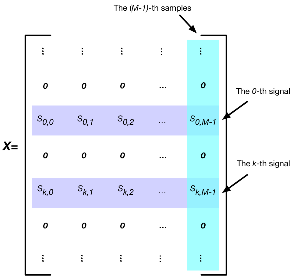
Refer to caption
Figure 2: The structure of sparse matrix 𝑿\boldsymbol{X}.

3.1 Sparse-Based Signal Model

Since the received signals are sparse in the spatial domain, we propose a sparse-based model to estimate the directions with unknown mutual coupling effect. In the sparse-based model, the dictionary matrix must be established first, so an over-complete dictionary matrix can be formulated by discretizing the signal direction uniformly in the spatial domain

𝑫≜[𝑸⁡(ζ0),𝑸⁡(ζ1),…,𝑸⁡(ζU−1)]∈ℂN×U​N,\displaystyle\boldsymbol{D}\triangleq\begin{bmatrix}\boldsymbol{Q}(\zeta_{0}),\boldsymbol{Q}(\zeta_{1}),\dots,\boldsymbol{Q}(\zeta_{U-1})\end{bmatrix}\in\mathbb{C}^{N\times UN}, (10)

where ζu\zeta_{u} denotes the uu-th discretized direction (u=0,1,…,U−1u=0,1,\dots,U-1), UU denotes the number of discretized directions, the grid size is defined as δ≜|ζu+1−ζu|\delta\triangleq|\zeta_{u+1}-\zeta_{u}|, and we use a vector to contain all the discretized directions 𝜻≜[ζ0,ζ1,…,ζU−1]\boldsymbol{\zeta}\triangleq\begin{bmatrix}\zeta_{0},\zeta_{1},\dots,\zeta_{U-1}\end{bmatrix}.

With the discretized directions and the system model in (9), a sparse-based on-grid direction finding model can be expressed as

𝒀=𝑫⁡(𝑿⊗𝒄)+𝑵,\displaystyle\boldsymbol{Y}=\boldsymbol{D}(\boldsymbol{X}\otimes\boldsymbol{c})+\boldsymbol{N}, (11)

where 𝑿\boldsymbol{X} is a sparse matrix

𝑿≜[𝒙0,𝒙1,…,𝒙M−1]∈ℂU×M.\displaystyle\boldsymbol{X}\triangleq\begin{bmatrix}\boldsymbol{x}_{0},\boldsymbol{x}_{1},\dots,\boldsymbol{x}_{M-1}\end{bmatrix}\in\mathbb{C}^{U\times M}. (12)

The structure of sparse matrix 𝑿\boldsymbol{X} is shown in Fig. 2, and the sparse vectors (𝒙0\boldsymbol{x}_{0}, 𝒙1\boldsymbol{x}_{1}, …\dots, 𝒙M−1\boldsymbol{x}_{M-1}) have the same support sets. When the direction of the kk-th received signal θk\theta_{k} is equal to the uku_{k}-th discretized direction ζuk\zeta_{u_{k}}, we have Xuk,m=Sk,mX_{u_{k},m}=S_{k,m}, so the uu-th row and mm-th column of 𝑿\boldsymbol{X} is

Xu,m={Sk,m,u=uk0,otherwise.\displaystyle X_{u,m}=\begin{cases}S_{k,m},&u=u_{k}\\ 0,&\text{otherwise}\end{cases}. (13)

The sparse-based model in (12) assumes that the directions of received signals are exactly on the discretized grids. However, in the practical direction finding system, when the direction θk\theta_{k} is not on the discretized grids, the direction θk\theta_{k} can be represented by ζuk\zeta_{u_{k}}, which is a grid nearest to θk\theta_{k}. Thus, the corresponding matrix 𝑸⁡(θk)\boldsymbol{Q}(\theta_{k}) in (2) can be approximated by

𝑸⁡(θk)≈𝑸⁡(ζuk)+(θk−ζuk)​𝛀​(ζuk),\displaystyle\boldsymbol{Q}(\theta_{k})\approx\boldsymbol{Q}(\zeta_{u_{k}})+(\theta_{k}-\zeta_{u_{k}})\boldsymbol{\Omega}(\zeta_{u_{k}}), (14)

where the first-order derivative is defined as 𝛀⁡(ζuk)≜∂𝑸⁡(ζ)∂ζ|ζ=ζuk\boldsymbol{\Omega}(\zeta_{u_{k}})\triangleq\left.\frac{\partial\boldsymbol{Q}(\zeta)}{\partial\zeta}\right|_{\zeta=\zeta_{u_{k}}}. For example, as shown in Fig. 3, the direction of signal sk​(t)s_{k}(t) is θk\theta_{k}, and the nearest grid is ζ3\zeta_{3}. Thus, the corresponding matrix 𝑸⁡(θk)\boldsymbol{Q}(\theta_{k}) in (14) can be written as 𝑸⁡(θk)≈𝑸⁡(ζ3)+(θk−ζ3)​𝛀​(ζ3)\boldsymbol{Q}(\theta_{k})\approx\boldsymbol{Q}(\zeta_{3})+(\theta_{k}-\zeta_{3})\boldsymbol{\Omega}(\zeta_{3}).

Refer to caption
Figure 3: The off-grid approximation for direction.

Therefore, with the approximation in (14), the received signal in (9) can be approximated by a sparse-based off-grid model

𝒀≈𝚿⁡(𝝂)​(𝑿⊗𝒄)+𝑵,\displaystyle\boldsymbol{Y}\approx\boldsymbol{\Psi}(\boldsymbol{\nu})(\boldsymbol{X}\otimes\boldsymbol{c})+\boldsymbol{N}, (15)

where 𝚿⁡(𝝂)≜𝑫+𝚵⁡(diag⁡{𝝂}⊗𝑰N)\boldsymbol{\Psi}(\boldsymbol{\nu})\triangleq\boldsymbol{D}+\boldsymbol{\Xi}\left(\operatorname{diag}\left\{\boldsymbol{\nu}\right\}\otimes\boldsymbol{I}_{N}\right), 𝚵≜[𝚵0,𝚵1,…,𝚵U−1]\boldsymbol{\Xi}\triangleq\begin{bmatrix}\boldsymbol{\Xi}_{0},\boldsymbol{\Xi}_{1},\dots,\boldsymbol{\Xi}_{U-1}\end{bmatrix}, and the uu-th submatrix of 𝚵\boldsymbol{\Xi} is denoted as 𝚵u≜𝛀⁡(ζu)\boldsymbol{\Xi}_{u}\triangleq\boldsymbol{\Omega}(\zeta_{u}). Additionally, a vector 𝝂∈ℝU×1\boldsymbol{\nu}\in\mathbb{R}^{U\times 1} is used to represent the off-grid directions, and the uu-th entry is

νu={θk−ζuk,u=uk0,otherwise.\displaystyle\nu_{u}=\begin{cases}\theta_{k}-\zeta_{u_{k}},&u=u_{k}\\ 0,&\text{otherwise}\end{cases}. (16)

Finally, an off-grid sparse-based model is formulated for the direction finding problem in (15). We will estimate the directions by reconstructing the sparse matrix 𝑿\boldsymbol{X}. The positions of non-zero entries in 𝑿\boldsymbol{X} indicate the directions of received signals. Simultaneously, the unknown parameters including the mutual coupling vector 𝒄\boldsymbol{c}, the noise variance σn2\sigma^{2}_{\text{n}} and the off-grid vector 𝝂\boldsymbol{\nu} will also be estimated.

3.2 Distribution Assumptions

Figure 4: Graphical model of sparse bayesian learning for direction estimation.

In the proposed DFSMC method, the sparse Bayesian learning theory is adopted, and the method is established based on the distribution assumptions of all the unknown parameters. We assume that the unknown parameters follow the following distributions:

  • •

    Noise 𝑵\boldsymbol{N}: Gaussian distribution;

  • •

    The precision of noise variance αn\alpha_{\text{n}}: Gamma distribution;

  • •

    Sparse matrix 𝑿\boldsymbol{X}: Gaussian distribution;

  • •

    The precision of signal variance 𝜾\boldsymbol{\iota}: Gamma distribution;

  • •

    Mutual coupling vector 𝒄\boldsymbol{c}: Gaussian distribution;

  • •

    The precision of mutual coupling variance ϑ\boldsymbol{\vartheta}: Gamma distribution;

  • •

    Off-grid vector 𝝂\boldsymbol{\nu}: Uniform distribution.

The relationships between all the unknown parameters are given in Fig. 4, and we will describe the distributions more clear in the following contents.

3.2.1 The distribution of noise

When the received signals are independent between different samples, with the assumption of circular symmetric white Gaussian noise, the distribution of noise can be expressed as

p⁡(𝑵|σn2)=∏m=0M−1𝒞​𝒩​(𝒏m|𝟎N×1,σn2​𝑰N),\displaystyle p(\boldsymbol{N}|\sigma^{2}_{\text{n}})=\prod^{M-1}_{m=0}\mathcal{CN}(\boldsymbol{n}_{m}|\boldsymbol{0}_{N\times 1},\sigma^{2}_{\text{n}}\boldsymbol{I}_{N}), (17)

where σn2\sigma^{2}_{\text{n}} denotes the noise variance, and the complex Gaussian distribution with the mean being 𝝁\boldsymbol{\mu} and the covariance matrix being 𝚺\boldsymbol{\Sigma} is expressed as

𝒞​𝒩​(𝒙|𝝁,𝚺)=1πN​det(𝚺)​e−(𝒙−𝝁)H​𝚺−1​(𝒙−𝝁).\displaystyle\mathcal{CN}(\boldsymbol{x}|\boldsymbol{\mu},\boldsymbol{\Sigma})=\frac{1}{\pi^{N}\det(\boldsymbol{\Sigma})}e^{-(\boldsymbol{x}-\boldsymbol{\mu})^{\text{H}}\boldsymbol{\Sigma}^{-1}(\boldsymbol{x}-\boldsymbol{\mu})}. (18)

3.2.2 The distribution of noise variance σn2\sigma_{\text{n}}^{2}

In this paper, the noise variance is unknown. Since the Gamma distribution is a conjugate prior of Gaussian distribution, the posterior distribution also follows a Gamma distribution. Therefore, using the Gamma distribution can simplify the following analysis. With the unknown noise variance σn2\sigma^{2}_{\text{n}}, we use a Gamma distribution to describe the precision of noise variance αn≜σn−2\alpha_{\text{n}}\triangleq\sigma^{-2}_{\text{n}}, and we have the following Gamma distribution

p⁡(αn)=g⁡(αn,a,b),\displaystyle p(\alpha_{\text{n}})=g(\alpha_{\text{n}};a,b), (19)

where aa and bb are the hyperparameters for αn\alpha_{\text{n}}, and g⁡(αn,a,b)≜Γ−1​(a)​ba​αna−1​e−b​αng(\alpha_{\text{n}};a,b)\triangleq\Gamma^{-1}(a)b^{a}\alpha_{\text{n}}^{a-1}e^{-b\alpha_{\text{n}}}, Γ⁡(a)≜∫0∞xa−1​e−x​𝑑x\Gamma(a)\triangleq\int^{\infty}_{0}x^{a-1}e^{-x}dx.

3.2.3 The distribution of sparse matrix

With the independent received signals 𝑺\boldsymbol{S} among samples, we can assume that the sparse matrix 𝑿\boldsymbol{X} follows a zero-mean Gaussian distribution

p⁡(𝑿|𝚲x)=∏m=0M−1𝒞​𝒩​(𝒙m|𝟎U×1,𝚲x),\displaystyle p(\boldsymbol{X}|\boldsymbol{\Lambda}_{\text{x}})=\prod_{m=0}^{M-1}\mathcal{CN}(\boldsymbol{x}_{m}|\boldsymbol{0}_{U\times 1},\boldsymbol{\Lambda}_{\text{x}}), (20)

where the covariance matrix 𝚲x∈ℝU×U\boldsymbol{\Lambda}_{\text{x}}\in\mathbb{R}^{U\times U} is a diagonal matrix with the uu-th diagonal entry being σx,u2\sigma^{2}_{\text{x},u}.

3.2.4 The distribution of signal variance

Similarity, with the unknown signal variance 𝚲x\boldsymbol{\Lambda}_{\text{x}}, we define the precision vector 𝜾≜[ι0,ι1,…,ιU−1]T\boldsymbol{\iota}\triangleq\begin{bmatrix}\iota_{0},\iota_{1},\dots,\iota_{U-1}\end{bmatrix}^{\text{T}}, where ιu≜σx,u−2\iota_{u}\triangleq\sigma^{-2}_{\text{x},u}, so 𝜾\boldsymbol{\iota} can be expressed by a Gamma prior

p⁡(𝜾,c,d)=∏u=0U−1g⁡(ιu,c,d),\displaystyle p(\boldsymbol{\iota};c,d)=\prod^{U-1}_{u=0}g(\iota_{u};c,d), (21)

where cc and dd are the hyperparmaters for 𝜾\boldsymbol{\iota}.

3.2.5 The distribution of mutual coupling vector

With the unknown mutual coupling vector, when the mutual coupling coefficients are independent between antennas, the distribution of mutual coupling vector 𝒄\boldsymbol{c} can be expressed as a Gaussian distribution

p⁡(𝒄|𝚲c)\displaystyle p(\boldsymbol{c}|\boldsymbol{\Lambda}_{\text{c}}) =∏n=0N−1𝒞​𝒩​(cn|0,𝚲c),\displaystyle=\prod^{N-1}_{n=0}\mathcal{CN}(c_{n}|0,\boldsymbol{\Lambda}_{\text{c}}), (22)

where the covariance matrix 𝚲c∈ℝN×N\boldsymbol{\Lambda}_{\text{c}}\in\mathbb{R}^{N\times N} is a diagonal matrix with the nn-th diagonal entry being σc,n2\sigma^{2}_{\text{c},n}.

3.2.6 The distribution of mutual coupling variance

By defining the precisions ϑ≜[ϑ0,ϑ1,…,ϑN−1]T\boldsymbol{\vartheta}\triangleq\begin{bmatrix}\vartheta_{0},\vartheta_{1},\dots,\vartheta_{N-1}\end{bmatrix}^{\text{T}} (ϑn≜σc,n−2\vartheta_{n}\triangleq\sigma^{-2}_{\text{c},n}), we use a Gamma distribution to describe the distribution of ϑ\boldsymbol{\vartheta}

p⁡(ϑ,e,f)\displaystyle p(\boldsymbol{\vartheta};e,f) =∏n=0N−1g⁡(ϑn,e,f),\displaystyle=\prod^{N-1}_{n=0}g(\vartheta_{n};e,f), (23)

where both ee and ff are the hyperparameters of ϑ\boldsymbol{\vartheta}.

3.2.7 The distribution of off-grid vector

We can assume that the off-grid vector 𝝂\boldsymbol{\nu} follows a uniform distribution, and the distribution of νu\nu_{u} can be expressed as

p⁡(νu,δ)=𝒰νu​([−12​δ,12​δ]),\displaystyle p(\nu_{u};\delta)=\mathcal{U}_{\nu_{u}}\left(\left[-\frac{1}{2}\delta,\frac{1}{2}\delta\right]\right), (24)

where the uniform distribution is defined as

𝒰x​([a,b])≜{1b−a,a≤x≤b0,otherwise.\displaystyle\mathcal{U}_{x}\left(\left[a,b\right]\right)\triangleq\begin{cases}\frac{1}{b-a},&a\leq x\leq b\\ 0,&\text{otherwise}\end{cases}. (25)

3.3 DFSMC method

With the distribution assumptions of unknown parameters, a novel direction finding method based on the SBL is proposed with the unknown mutual coupling effect, named DFSMC. In the SBL-based method, the posterior probabilities for all the unknown parameters are theoretically derived.

To estimate the directions, we formulate the following problem to maximize the posterior probability

℘^=arg⁡max℘⁡p⁡(℘|𝒀),\displaystyle\hat{\wp}=\arg\max_{\wp}p(\wp|\boldsymbol{Y}), (26)

where a set ℘≜{𝑿,𝝂,𝒄,σn2,𝜾,ϑ}\wp\triangleq\left\{\boldsymbol{X},\boldsymbol{\nu},\boldsymbol{c},\sigma^{2}_{\text{n}},\boldsymbol{\iota},\boldsymbol{\vartheta}\right\} is used to contain all the unknown parameters. However, the problem (26) is too complex and cannot be solved directly. The expectation maximum (EM)-based method is used to realize the proposed DFSMC method. Additionally, with the received signal 𝒀\boldsymbol{Y}, the joint distribution with unknown parameters can be expressed as

p⁡(𝒀,℘)\displaystyle p(\boldsymbol{Y},\wp) =p⁡(𝒀|℘)​p​(𝑿|𝜾)​p​(𝒄|ϑ)​p​(αn)​p​(𝜾)​p​(ϑ)​p​(𝝂).\displaystyle=p(\boldsymbol{Y}|\wp)p(\boldsymbol{X}|\boldsymbol{\iota})p(\boldsymbol{c}|\boldsymbol{\vartheta})p(\alpha_{\text{n}})p(\boldsymbol{\iota})p(\boldsymbol{\vartheta})p(\boldsymbol{\nu}). (27)

The details to estimate all unknown parameters are given as follows.

3.3.1 The sparse matrix

Given the received signal 𝒀\boldsymbol{Y} and the parameters (℘\𝑿)(\wp\backslash\boldsymbol{X}) excepting 𝑿\boldsymbol{X}, the the posterior of 𝑿\boldsymbol{X} can be expressed as

p⁡(𝑿|𝒀,𝝂,𝒄,αn,𝜾,ϑ)\displaystyle p(\boldsymbol{X}|\boldsymbol{Y},\boldsymbol{\nu},\boldsymbol{c},\alpha_{\text{n}},\boldsymbol{\iota},\boldsymbol{\vartheta}) =p⁡(𝒀|℘)​p​(𝑿|𝜾)p⁡(𝒀|𝝂,𝒄,αn,𝜾,ϑ)∝p⁡(𝒀|℘)​p​(𝑿|𝜾),\displaystyle=\frac{p(\boldsymbol{Y}|\wp)p(\boldsymbol{X}|\boldsymbol{\iota})}{p(\boldsymbol{Y}|\boldsymbol{\nu},\boldsymbol{c},\alpha_{\text{n}},\boldsymbol{\iota},\boldsymbol{\vartheta})}\propto p(\boldsymbol{Y}|\wp)p(\boldsymbol{X}|\boldsymbol{\iota}), (28)

where both p⁡(𝒀|℘)p(\boldsymbol{Y}|\wp) and p⁡(𝑿|𝜾)p(\boldsymbol{X}|\boldsymbol{\iota}) follow Gaussian distributions, and can be calculated as

p⁡(𝒀|℘)\displaystyle p(\boldsymbol{Y}|\wp) =∏m=0M−1αnNπN​e−αn​‖𝒚m−𝚿⁡(𝝂)​(𝒙m⊗𝒄)‖22,\displaystyle=\prod^{M-1}_{m=0}\frac{\alpha_{\text{n}}^{N}}{\pi^{N}}e^{-\alpha_{\text{n}}\|\boldsymbol{y}_{m}-\boldsymbol{\Psi}(\boldsymbol{\nu})(\boldsymbol{x}_{m}\otimes\boldsymbol{c})\|^{2}_{2}}, (29)
p⁡(𝑿|𝜾)\displaystyle p(\boldsymbol{X}|\boldsymbol{\iota}) =∏m=0M−1(∏u=0U−1ιu)​1πU​e−𝒙mH​diag⁡{𝜾}​𝒙m.\displaystyle=\prod_{m=0}^{M-1}\left(\prod^{U-1}_{u=0}\iota_{u}\right)\frac{1}{\pi^{U}}e^{-\boldsymbol{x}^{\text{H}}_{m}\operatorname{diag}\{\boldsymbol{\iota}\}\boldsymbol{x}_{m}}. (30)

Therefore, the posterior of 𝑿\boldsymbol{X} is also a Gaussian function

p⁡(𝑿|𝒀,𝝂,𝒄,αn,𝜾,ϑ)=∏m=0M−1𝒞​𝒩​(𝒙m|𝝁m,𝚺X),\displaystyle p(\boldsymbol{X}|\boldsymbol{Y},\boldsymbol{\nu},\boldsymbol{c},\alpha_{\text{n}},\boldsymbol{\iota},\boldsymbol{\vartheta})=\prod^{M-1}_{m=0}\mathcal{CN}(\boldsymbol{x}_{m}|\boldsymbol{\mu}_{m},\boldsymbol{\Sigma}_{\text{X}}), (31)

where the mean 𝝁m\boldsymbol{\mu}_{m} and covariance matrix 𝚺X\boldsymbol{\Sigma}_{\text{X}} are obtained from (29) and (30) as

𝝁m\displaystyle\boldsymbol{\mu}_{m} =αnH​𝚺XH​𝔗H​(𝝂,𝒄)​𝒚m,\displaystyle=\alpha_{\text{n}}^{\text{H}}\boldsymbol{\Sigma}^{\text{H}}_{\text{X}}\mathfrak{T}^{H}(\boldsymbol{\nu},\boldsymbol{c})\boldsymbol{y}_{m}, (32)
𝚺X\displaystyle\boldsymbol{\Sigma}_{\text{X}} =[αn​𝔗H​(𝝂,𝒄)​𝔗​(𝝂,𝒄)+diag⁡{𝜾}]−1,\displaystyle=\left[\alpha_{\text{n}}\mathfrak{T}^{H}(\boldsymbol{\nu},\boldsymbol{c})\mathfrak{T}(\boldsymbol{\nu},\boldsymbol{c})+\operatorname{diag}\{\boldsymbol{\iota}\}\right]^{-1}, (33)

and we define the following function

𝔗⁡(𝝂,𝒄)≜𝚿⁡(𝝂)​(𝑰U⊗𝒄).\displaystyle\mathfrak{T}(\boldsymbol{\nu},\boldsymbol{c})\triangleq\boldsymbol{\Psi}(\boldsymbol{\nu})(\boldsymbol{I}_{U}\otimes\boldsymbol{c}). (34)

Additionally, to simplify the notations, the uu-th entry of 𝝁m\boldsymbol{\mu}_{m} is denoted as μu,m\mu_{u,m}, and we can collect all the mean 𝝁m\boldsymbol{\mu}_{m} as a matrix 𝝁≜[𝝁0,𝝁1,…,𝝁M−1]\boldsymbol{\mu}\triangleq\begin{bmatrix}\boldsymbol{\mu}_{0},\boldsymbol{\mu}_{1},\dots,\boldsymbol{\mu}_{M-1}\end{bmatrix}.

To estimate the other unknown parameters ℘\𝑿\wp\backslash\boldsymbol{X}, with (27), we can formulate the following likelihood function

ℒ(𝝂,𝒄,αn,𝜾,ϑ)=ℰ{\displaystyle\mathcal{L}(\boldsymbol{\nu},\boldsymbol{c},\alpha_{\text{n}},\boldsymbol{\iota},\boldsymbol{\vartheta})=\mathcal{E}\big\{ lnp(𝒀|℘)p(𝑿|𝜾)p(𝒄|ϑ)p(αn)p(𝜾)p(ϑ)p(𝝂)}.\displaystyle\ln p(\boldsymbol{Y}|\wp)p(\boldsymbol{X}|\boldsymbol{\iota})p(\boldsymbol{c}|\boldsymbol{\vartheta})p(\alpha_{\text{n}})p(\boldsymbol{\iota})p(\boldsymbol{\vartheta})p(\boldsymbol{\nu})\big\}. (35)

where we just use ℰ​{⋅}\mathcal{E}\{\cdot\} to represent ℰ𝑿|𝒀,𝝂,αn,𝜾,ϑ​{⋅}\mathcal{E}_{\boldsymbol{X}|\boldsymbol{Y},\boldsymbol{\nu},\alpha_{\text{n}},\boldsymbol{\iota},\boldsymbol{\vartheta}}\{\cdot\}. Thus, the EM-based method can be used to estimate ℘\𝑿\wp\backslash\boldsymbol{X}, and the details are given in the following contents. Additionally, the derivatives for the complex vector and matrix are given as the following lemma.

Lemma \thetheorem

With both the complex vectors (𝐮∈ℂP×1\boldsymbol{u}\in\mathbb{C}^{P\times 1}, 𝐯∈ℂP×1\boldsymbol{v}\in\mathbb{C}^{P\times 1}) and the complex matrix 𝐀∈ℂM×P\boldsymbol{A}\in\mathbb{C}^{M\times P} being the function of a complex vector 𝐱∈ℂN×1\boldsymbol{x}\in\mathbb{C}^{N\times 1}, the following derivations can be obtained

∂𝒖H​𝒗∂𝒙=𝒗T​∂(𝒖∗)∂𝒙+𝒖H​∂𝒗∂𝒙,\displaystyle\frac{\partial\boldsymbol{u}^{\text{H}}\boldsymbol{v}}{\partial\boldsymbol{x}}=\boldsymbol{v}^{\text{T}}\frac{\partial(\boldsymbol{u}^{*})}{\partial\boldsymbol{x}}+\boldsymbol{u}^{\text{H}}\frac{\partial\boldsymbol{v}}{\partial\boldsymbol{x}}, (36)
∂𝑨​𝒖∂𝒙=[∂𝑨∂x0​𝒖+𝑨​∂𝒖∂x0,…,∂𝑨∂xn​𝒖+𝑨​∂𝒖∂xn,…].\displaystyle\frac{\partial\boldsymbol{Au}}{\partial\boldsymbol{x}}=\begin{bmatrix}\frac{\partial\boldsymbol{A}}{\partial x_{0}}\boldsymbol{u}+\boldsymbol{A}\frac{\partial\boldsymbol{u}}{\partial x_{0}},\ldots,\frac{\partial\boldsymbol{A}}{\partial x_{n}}\boldsymbol{u}+\boldsymbol{A}\frac{\partial\boldsymbol{u}}{\partial x_{n}},\ldots\end{bmatrix}. (37)
Proof.

See: Appendix A. ∎

3.3.2 The mutual coupling vector

Ignoring terms independent thereof in ℒ⁡(𝝂,𝒄,αn,𝜾,ϑ)\mathcal{L}(\boldsymbol{\nu},\boldsymbol{c},\alpha_{\text{n}},\boldsymbol{\iota},\boldsymbol{\vartheta}), we can obtain the following likelihood function for the mutual coupling vector 𝒄\boldsymbol{c}

ℒ\displaystyle\mathcal{L} (𝒄)=ℰ⁡{ln⁡p⁡(𝒀|𝑿,𝝂,𝒄,αn)​p​(𝒄|ϑ)}\displaystyle(\boldsymbol{\boldsymbol{c}})=\mathcal{E}\left\{\ln p(\boldsymbol{Y}|\boldsymbol{X},\boldsymbol{\nu},\boldsymbol{c},\alpha_{\text{n}})p(\boldsymbol{c}|\boldsymbol{\vartheta})\right\}
=ℰ{ln∏m=0M−1𝒞𝒩(𝒚m|𝚿(𝝂)(𝒙m⊗𝒄),αn−1𝑰N)}+ln∏n=0N−1𝒞𝒩(cn|0,ϑn−1)\displaystyle=\mathcal{E}\left\{\ln\prod^{M-1}_{m=0}\mathcal{CN}(\boldsymbol{y}_{m}|\boldsymbol{\Psi}(\boldsymbol{\nu})(\boldsymbol{x}_{m}\otimes\boldsymbol{c}),\alpha^{-1}_{\text{n}}\boldsymbol{I}_{N})\right\}+\ln\prod^{N-1}_{n=0}\mathcal{CN}(c_{n}|0,\vartheta^{-1}_{n}) (38)
∝−αn​M​𝒢1​(𝒄,𝝂)−∑m=0M−1αn​𝒢2,m​(𝒄,𝝂)−𝒢3​(𝒄),\displaystyle\propto-\alpha_{\text{n}}M\mathcal{G}_{1}(\boldsymbol{c},\boldsymbol{\nu})-\sum^{M-1}_{m=0}\alpha_{\text{n}}\mathcal{G}_{2,m}(\boldsymbol{c},\boldsymbol{\nu})-\mathcal{G}_{3}(\boldsymbol{c}),

where we have

ℰ⁡{ln⁡p⁡(𝒀|𝑿,𝝂,𝒄,αn)}=\displaystyle\mathcal{E}\left\{\ln p(\boldsymbol{Y}|\boldsymbol{X},\boldsymbol{\nu},\boldsymbol{c},\alpha_{\text{n}})\right\}= M​N​ln⁡αnπ−αn​M​𝒢1​(𝒄,𝝂)−∑m=0M−1αn​𝒢2,m​(𝒄,𝝂),\displaystyle MN\ln\frac{\alpha_{\text{n}}}{\pi}-\alpha_{\text{n}}M\mathcal{G}_{1}(\boldsymbol{c},\boldsymbol{\nu})-\sum^{M-1}_{m=0}\alpha_{\text{n}}\mathcal{G}_{2,m}(\boldsymbol{c},\boldsymbol{\nu}), (39)

and 𝒢1​(𝒄,𝝂)≜Tr⁡{𝔗H​(𝝂,𝒄)​𝔗​(𝝂,𝒄)​𝚺X}\mathcal{G}_{1}(\boldsymbol{c},\boldsymbol{\nu})\triangleq\operatorname{Tr}\left\{\mathfrak{T}^{H}(\boldsymbol{\nu},\boldsymbol{c})\mathfrak{T}(\boldsymbol{\nu},\boldsymbol{c})\boldsymbol{\Sigma}_{\text{X}}\right\}, 𝒢2,m​(𝒄,𝝂)≜‖𝒚m−𝚿⁡(𝝂)​(𝝁m⊗𝒄)‖22\mathcal{G}_{2,m}(\boldsymbol{c},\boldsymbol{\nu})\triangleq\|\boldsymbol{y}_{m}-\boldsymbol{\Psi}(\boldsymbol{\nu})(\boldsymbol{\mu}_{m}\otimes\boldsymbol{c})\|^{2}_{2}, 𝒢3​(𝒄)≜∑n=0N−1ϑn​|cn|2\mathcal{G}_{3}(\boldsymbol{c})\triangleq\sum^{N-1}_{n=0}\vartheta_{n}|c_{n}|^{2}.

To estimate the mutual coupling vector 𝒄\boldsymbol{c}, we can maximize the likelihood function ℒ⁡(𝒄)\mathcal{L}(\boldsymbol{\boldsymbol{c}}), and we have

𝒄^=arg⁡max𝒄⁡ℒ⁡(𝒄).\displaystyle\hat{\boldsymbol{c}}=\arg\max_{\boldsymbol{c}}\mathcal{L}(\boldsymbol{c}). (40)

Therefore, by setting ∂ℒ⁡(𝒄)∂𝒄=𝟎\frac{\partial\mathcal{L}(\boldsymbol{c})}{\partial\boldsymbol{c}}=\boldsymbol{0}, the mutual coupling vector can be obtained. We can calculate

∂ℒ⁡(𝒄)∂𝒄\displaystyle\frac{\partial\mathcal{L}(\boldsymbol{c})}{\partial\boldsymbol{c}} =−αn​M​∂𝒢1​(𝒄,𝝂)∂𝒄−∑m=0M−1αn​∂𝒢2,m​(𝒄,𝝂)∂𝒄−∂𝒢3​(𝒄)∂𝒄.\displaystyle=-\alpha_{\text{n}}M\frac{\partial\mathcal{G}_{1}(\boldsymbol{c},\boldsymbol{\nu})}{\partial\boldsymbol{c}}-\sum^{M-1}_{m=0}\alpha_{\text{n}}\frac{\partial\mathcal{G}_{2,m}(\boldsymbol{c},\boldsymbol{\nu})}{\partial\boldsymbol{c}}-\frac{\partial\mathcal{G}_{3}(\boldsymbol{c})}{\partial\boldsymbol{c}}. (41)

In (41), ∂𝒢1​(𝒄,𝝂)∂𝒄\frac{\partial\mathcal{G}_{1}(\boldsymbol{c},\boldsymbol{\nu})}{\partial\boldsymbol{c}}, ∂𝒢2,m​(𝒄,𝝂)∂𝒄\frac{\partial\mathcal{G}_{2,m}(\boldsymbol{c},\boldsymbol{\nu})}{\partial\boldsymbol{c}} and ∂𝒢3​(𝒄)∂𝒄\frac{\partial\mathcal{G}_{3}(\boldsymbol{c})}{\partial\boldsymbol{c}} can be calculated as follows.

  • •

    For ∂𝒢1​(𝐜,𝛎)∂𝐜\frac{\partial\mathcal{G}_{1}(\boldsymbol{c},\boldsymbol{\nu})}{\partial\boldsymbol{c}}: With the derivations of complex vector and matrix in Appendix A, ∂𝒢1​(𝒄,𝝂)∂𝒄\frac{\partial\mathcal{G}_{1}(\boldsymbol{c},\boldsymbol{\nu})}{\partial\boldsymbol{c}} is a row vector, and the nn-th entry can be calculated as

    [∂𝒢1​(𝒄,𝝂)∂𝒄]n=Tr⁡{∂𝔗H​(𝝂,𝒄)​𝔗​(𝝂,𝒄)​𝚺X∂cn}.\displaystyle\left[\frac{\partial\mathcal{G}_{1}(\boldsymbol{c},\boldsymbol{\nu})}{\partial\boldsymbol{c}}\right]_{n}=\operatorname{Tr}\left\{\frac{\partial\mathfrak{T}^{H}(\boldsymbol{\nu},\boldsymbol{c})\mathfrak{T}(\boldsymbol{\nu},\boldsymbol{c})\boldsymbol{\Sigma}_{\text{X}}}{\partial c_{n}}\right\}. (42)

    Additionally, we can calculate

    ∂𝔗H​(𝝂,𝒄)​𝔗​(𝝂,𝒄)​𝚺X∂cn=∂(𝑰U⊗𝒄)H∂cn𝚿H(𝝂)𝔗(𝝂,𝒄)𝚺X]+𝔗H(𝝂,𝒄)𝚿(𝝂)∂(𝑰U⊗𝒄)∂cn𝚺X\displaystyle\frac{\partial\mathfrak{T}^{H}(\boldsymbol{\nu},\boldsymbol{c})\mathfrak{T}(\boldsymbol{\nu},\boldsymbol{c})\boldsymbol{\Sigma}_{\text{X}}}{\partial c_{n}}=\frac{\partial(\boldsymbol{I}_{U}\otimes\boldsymbol{c})^{\text{H}}}{\partial c_{n}}\boldsymbol{\Psi}^{\text{H}}(\boldsymbol{\nu})\mathfrak{T}(\boldsymbol{\nu},\boldsymbol{c})\boldsymbol{\Sigma}_{\text{X}}]+\mathfrak{T}^{H}(\boldsymbol{\nu},\boldsymbol{c})\boldsymbol{\Psi}(\boldsymbol{\nu})\frac{\partial(\boldsymbol{I}_{U}\otimes\boldsymbol{c})}{\partial c_{n}}\boldsymbol{\Sigma}_{\text{X}}
    =𝔗H​(𝝂,𝒄)​𝚿​(𝝂)​(𝑰U⊗∂𝒄∂cn)​𝚺X=𝔗H​(𝝂,𝒄)​𝔗​(𝝂,𝒆nN)​𝚺X,\displaystyle=\mathfrak{T}^{H}(\boldsymbol{\nu},\boldsymbol{c})\boldsymbol{\Psi}(\boldsymbol{\nu})\left(\boldsymbol{I}_{U}\otimes\frac{\partial\boldsymbol{c}}{\partial c_{n}}\right)\boldsymbol{\Sigma}_{\text{X}}=\mathfrak{T}^{H}(\boldsymbol{\nu},\boldsymbol{c})\mathfrak{T}(\boldsymbol{\nu},\boldsymbol{e}^{N}_{n})\boldsymbol{\Sigma}_{\text{X}}, (43)

    where 𝒆nN\boldsymbol{e}^{N}_{n} is a N×1N\times 1 vector with the nn-th entry being 11 and other entries being 00. Therefore, the the nn-th entry in (42) can be simplified as

    [∂𝒢1​(𝒄,𝝂)∂𝒄]n\displaystyle\left[\frac{\partial\mathcal{G}_{1}(\boldsymbol{c},\boldsymbol{\nu})}{\partial\boldsymbol{c}}\right]_{n} =𝒄H​(∑p=0U−1∑k=0U−1𝚿pH​(𝝂)​𝚿k​(𝝂)​ΣX,k,p)​𝒆nN,\displaystyle=\boldsymbol{c}^{\text{H}}\left(\sum_{p=0}^{U-1}\sum_{k=0}^{U-1}\boldsymbol{\Psi}^{\text{H}}_{p}(\boldsymbol{\nu})\boldsymbol{\Psi}_{k}(\boldsymbol{\nu})\Sigma_{\text{X},k,p}\right)\boldsymbol{e}^{N}_{n}, (44)

    and we finally have the derivation of 𝒢1​(𝒄,𝝂)\mathcal{G}_{1}(\boldsymbol{c},\boldsymbol{\nu}) as

    ∂𝒢1​(𝒄,𝝂)∂𝒄\displaystyle\frac{\partial\mathcal{G}_{1}(\boldsymbol{c},\boldsymbol{\nu})}{\partial\boldsymbol{c}} =𝒄H​(∑p=0U−1∑k=0U−1𝚿pH​(𝝂)​𝚿k​(𝝂)​ΣX,k,p).\displaystyle=\boldsymbol{c}^{\text{H}}\left(\sum_{p=0}^{U-1}\sum_{k=0}^{U-1}\boldsymbol{\Psi}^{\text{H}}_{p}(\boldsymbol{\nu})\boldsymbol{\Psi}_{k}(\boldsymbol{\nu})\Sigma_{\text{X},k,p}\right).
  • •

    ∂𝒢2,m​(𝒄,𝝂)∂𝒄\frac{\partial\mathcal{G}_{2,m}(\boldsymbol{c},\boldsymbol{\nu})}{\partial\boldsymbol{c}} can be simplified as

    ∂𝒢2,m​(𝒄,𝝂)∂𝒄\displaystyle\frac{\partial\mathcal{G}_{2,m}(\boldsymbol{c},\boldsymbol{\nu})}{\partial\boldsymbol{c}} =−[𝒚m−𝚿⁡(𝝂)​(𝝁m⊗𝒄)]H​𝚿​(𝝂)​∂𝝁m⊗𝒄∂𝒄\displaystyle=-[\boldsymbol{y}_{m}-\boldsymbol{\Psi}(\boldsymbol{\nu})(\boldsymbol{\mu}_{m}\otimes\boldsymbol{c})]^{\text{H}}\boldsymbol{\Psi}(\boldsymbol{\nu})\frac{\partial\boldsymbol{\mu}_{m}\otimes\boldsymbol{c}}{\partial\boldsymbol{c}}
    =−[𝒚m−𝚿⁡(𝝂)​(𝝁m⊗𝒄)]H​𝚿​(𝝂)​(𝝁m⊗𝑰N).\displaystyle=-[\boldsymbol{y}_{m}-\boldsymbol{\Psi}(\boldsymbol{\nu})(\boldsymbol{\mu}_{m}\otimes\boldsymbol{c})]^{\text{H}}\boldsymbol{\Psi}(\boldsymbol{\nu})(\boldsymbol{\mu}_{m}\otimes\boldsymbol{I}_{N}). (45)
  • •

    ∂𝒢3​(𝒄)∂𝒄\frac{\partial\mathcal{G}_{3}(\boldsymbol{c})}{\partial\boldsymbol{c}} can be simplified as ∂𝒢3​(𝒄)∂𝒄=𝒄H​diag⁡{ϑ}\frac{\partial\mathcal{G}_{3}(\boldsymbol{c})}{\partial\boldsymbol{c}}=\boldsymbol{c}^{H}\operatorname{diag}\{\boldsymbol{\vartheta}\}.

Therefore, with (41), the mutual coupling vector can be finally estimated as

𝒄^=𝑯−1​𝒛,\displaystyle\hat{\boldsymbol{c}}=\boldsymbol{H}^{-1}\boldsymbol{z}, (46)

where

𝑯\displaystyle\boldsymbol{H} =∑m=0M−1αn​𝔓H​(𝝂,𝝁m)​𝔓​(𝝂,𝝁m)+αn​M​(∑p=0U−1∑k=0U−1𝚿pH​(𝝂)​𝚿k​(𝝂)​ΣX,k,p)H+diag⁡{ϑ},\displaystyle=\sum^{M-1}_{m=0}\alpha_{\text{n}}\mathfrak{P}^{H}(\boldsymbol{\nu},\boldsymbol{\mu}_{m})\mathfrak{P}(\boldsymbol{\nu},\boldsymbol{\mu}_{m})+\alpha_{\text{n}}M\left(\sum_{p=0}^{U-1}\sum_{k=0}^{U-1}\boldsymbol{\Psi}^{\text{H}}_{p}(\boldsymbol{\nu})\boldsymbol{\Psi}_{k}(\boldsymbol{\nu})\Sigma_{\text{X},k,p}\right)^{\text{H}}+\operatorname{diag}\{\boldsymbol{\vartheta}\}, (47)
𝒛\displaystyle\boldsymbol{z} =∑m=0M−1αn​𝔓H​(𝝂,𝝁m)​𝒚m,\displaystyle=\sum^{M-1}_{m=0}\alpha_{\text{n}}\mathfrak{P}^{H}(\boldsymbol{\nu},\boldsymbol{\mu}_{m})\boldsymbol{y}_{m}, (48)

and we define 𝔓⁡(𝝂,𝝁m)≜𝚿⁡(𝝂)​(𝝁m⊗𝑰N)\mathfrak{P}(\boldsymbol{\nu},\boldsymbol{\mu}_{m})\triangleq\boldsymbol{\Psi}(\boldsymbol{\nu})(\boldsymbol{\mu}_{m}\otimes\boldsymbol{I}_{N}).

3.3.3 For the precision of signal variance

Ignoring terms independent thereof in ℒ⁡(𝝂,𝒄,αn,𝜾,ϑ)\mathcal{L}(\boldsymbol{\nu},\boldsymbol{c},\alpha_{\text{n}},\boldsymbol{\iota},\boldsymbol{\vartheta}), we can obtain the likelihood function of 𝜾\boldsymbol{\iota} as

ℒ⁡(𝜾)=\displaystyle\mathcal{L}(\boldsymbol{\iota})= ℰ{lnp(𝑿|𝜾)p(𝜾)}=ℰ{ln∏m=0M−1𝒞𝒩(𝒙m|𝟎U×1,𝚲x)}+ln∏u=0U−1g(ιu;c,d).\displaystyle\mathcal{E}\left\{\ln p(\boldsymbol{X}|\boldsymbol{\iota})p(\boldsymbol{\iota})\right\}=\mathcal{E}\left\{\ln\prod_{m=0}^{M-1}\mathcal{CN}(\boldsymbol{x}_{m}|\boldsymbol{0}_{U\times 1},\boldsymbol{\Lambda}_{\text{x}})\right\}+\ln\prod^{U-1}_{u=0}g(\iota_{u};c,d). (49)

Then, the precision of signal variance can be estimated by 𝜾^=arg⁡max𝜾⁡ℒ⁡(𝜾)\hat{\boldsymbol{\iota}}=\arg\max_{\boldsymbol{\iota}}\mathcal{L}(\boldsymbol{\iota}).

By setting ∂ℒ⁡(𝜾)∂𝜾=0\frac{\partial\mathcal{L}(\boldsymbol{\iota})}{\partial\boldsymbol{\iota}}=0, the uu-th entry of 𝜾\boldsymbol{\iota} can be obtained as

ι^u=M+c−1d+M​ΣX,u,u+∑m=0M−1|μu,m|2.\displaystyle\hat{\iota}_{u}=\frac{M+c-1}{d+M\Sigma_{\text{X},u,u}+\sum_{m=0}^{M-1}|\mu_{u,m}|^{2}}. (50)

In the iterative algorithm, (50) can be rewritten as

ι^ui+1≈M−1−ι^ui​∑m=0M−1|μu,m|2d+M​ΣX,u,u,\displaystyle\hat{\iota}^{i+1}_{u}\approx\frac{M-1-\hat{\iota}^{i}_{u}\sum_{m=0}^{M-1}|\mu_{u,m}|^{2}}{d+M\Sigma_{\text{X},u,u}}, (51)

where ι^ui+1\hat{\iota}^{i+1}_{u} and ι^ui\hat{\iota}^{i}_{u} are the esitmated results at the (i+1)(i+1)-th and the ii-th iterations, respectively.

3.3.4 For αn\alpha_{\text{n}}

Ignoring terms independent thereof in ℒ⁡(𝝂,𝒄,αn,𝜾,ϑ)\mathcal{L}(\boldsymbol{\nu},\boldsymbol{c},\alpha_{\text{n}},\boldsymbol{\iota},\boldsymbol{\vartheta}), we can obtain the likelihood function

ℒ⁡(αn)\displaystyle\mathcal{L}(\alpha_{\text{n}}) =ℰ⁡{ln⁡p⁡(𝒀|𝑿,𝝂,𝒄,αn)​p​(αn)}\displaystyle=\mathcal{E}\left\{\ln p(\boldsymbol{Y}|\boldsymbol{X},\boldsymbol{\nu},\boldsymbol{c},\alpha_{\text{n}})p(\alpha_{\text{n}})\right\}
=ℰ{ln∏m=0M−1𝒞𝒩(𝒚m|𝚿(𝝂)(𝒙m⊗𝒄),σn2𝑰)}+lng(αn;a,b).\displaystyle=\mathcal{E}\left\{\ln\prod_{m=0}^{M-1}\mathcal{CN}\left(\boldsymbol{y}_{m}|\boldsymbol{\Psi}(\boldsymbol{\nu})(\boldsymbol{x}_{m}\otimes\boldsymbol{c}),\sigma^{2}_{\text{n}}\boldsymbol{I}\right)\right\}+\ln g(\alpha_{\text{n}};a,b). (52)

The precision of noise variance can be estimated by

α^n=arg⁡maxαn⁡ℒ⁡(αn).\displaystyle\hat{\alpha}_{\text{n}}=\arg\max_{\alpha_{\text{n}}}\mathcal{L}(\alpha_{\text{n}}). (53)

By setting ∂ℒ⁡(αn)∂αn=0\frac{\partial\mathcal{L}(\alpha_{\text{n}})}{\partial\alpha_{\text{n}}}=0, we can obtain

α^n\displaystyle\hat{\alpha}_{\text{n}} =M​N+a−1M​𝒢1​(𝒄,𝝂)+∑m=0M−1𝒢2,m​(𝒄,𝝂)+b.\displaystyle=\frac{MN+a-1}{M\mathcal{G}_{1}(\boldsymbol{c},\boldsymbol{\nu})+\sum^{M-1}_{m=0}\mathcal{G}_{2,m}(\boldsymbol{c},\boldsymbol{\nu})+b}. (54)

In the iterative algorithm, (54) can be rewritten as

α^ni+1≈M​N−1−α^ni​∑m=0M−1𝒢2,m​(𝒄,𝝂)M​𝒢1​(𝒄,𝝂)+b.,\displaystyle\hat{\alpha}^{i+1}_{\text{n}}\approx\frac{MN-1-\hat{\alpha}^{i}_{\text{n}}\sum^{M-1}_{m=0}\mathcal{G}_{2,m}(\boldsymbol{c},\boldsymbol{\nu})}{M\mathcal{G}_{1}(\boldsymbol{c},\boldsymbol{\nu})+b}., (55)

where α^ni+1\hat{\alpha}^{i+1}_{\text{n}} and α^ni\hat{\alpha}^{i}_{\text{n}} are the esitmated results at the (i+1)(i+1)-th and the ii-th iterations, respectively.

3.3.5 For the precision of mutual coupling variance

Ignoring terms independent thereof in ℒ⁡(𝝂,𝒄,αn,𝜾,ϑ)\mathcal{L}(\boldsymbol{\nu},\boldsymbol{c},\alpha_{\text{n}},\boldsymbol{\iota},\boldsymbol{\vartheta}), we can obtain the likelihood function

ℒ⁡(ϑ)\displaystyle\mathcal{L}(\boldsymbol{\vartheta}) =ℰ{lnp(𝒄|ϑ)p(ϑ)}=ℰ{ln∏n=0N−1𝒞𝒩(cn|0,ϑn−1)}+ln∏n=0N−1g(ϑn;e,f).\displaystyle=\mathcal{E}\left\{\ln p(\boldsymbol{c}|\boldsymbol{\vartheta})p(\boldsymbol{\vartheta})\right\}=\mathcal{E}\left\{\ln\prod^{N-1}_{n=0}\mathcal{CN}(c_{n}|0,\vartheta_{n}^{-1})\right\}+\ln\prod^{N-1}_{n=0}g(\vartheta_{n};e,f). (56)

The precision of mutual coupling variance can be estimated by ϑ^=arg⁡maxϑ⁡ℒ⁡(ϑ)\hat{\boldsymbol{\vartheta}}=\arg\max_{\boldsymbol{\vartheta}}\mathcal{L}(\boldsymbol{\vartheta}).

By setting ∂ℒ⁡(ϑ)∂ϑ=𝟎\frac{\partial\mathcal{L}(\boldsymbol{\vartheta})}{\partial\boldsymbol{\vartheta}}=\boldsymbol{0}, we can obtain the nn-th entry of ϑ\boldsymbol{\vartheta} as

ϑ^n≈1f+cnH​cn.\displaystyle\hat{\vartheta}_{n}\approx\frac{1}{f+c_{n}^{\text{H}}c_{n}}. (57)

3.3.6 For the off-grid vector

Ignoring terms independent thereof in ℒ⁡(𝝂,𝒄,αn,𝜾,ϑ)\mathcal{L}(\boldsymbol{\nu},\boldsymbol{c},\alpha_{\text{n}},\boldsymbol{\iota},\boldsymbol{\vartheta}), we can obtain the likelihood function

ℒ⁡(𝝂)\displaystyle\mathcal{L}(\boldsymbol{\nu}) =ℰ⁡{ln⁡p⁡(𝒀|𝑿,𝝂,𝒄,αn)​p​(𝝂)}∝−M​𝒢1​(𝒄,𝝂)−∑m=0M−1𝒢2,m​(𝒄,𝝂).\displaystyle=\mathcal{E}\left\{\ln p(\boldsymbol{Y}|\boldsymbol{X},\boldsymbol{\nu},\boldsymbol{c},\alpha_{n})p(\boldsymbol{\nu})\right\}\propto-M\mathcal{G}_{1}(\boldsymbol{c},\boldsymbol{\nu})-\sum^{M-1}_{m=0}\mathcal{G}_{2,m}(\boldsymbol{c},\boldsymbol{\nu}). (58)

The off-grid vector can be estimated by

𝝂^=arg⁡max𝝂⁡ℒ⁡(𝝂).\displaystyle\hat{\boldsymbol{\nu}}=\arg\max_{\boldsymbol{\nu}}\mathcal{L}(\boldsymbol{\nu}). (59)

Then, ∂𝒢1​(𝒄,𝝂)∂𝝂∈ℝ1×U\frac{\partial\mathcal{G}_{1}(\boldsymbol{c},\boldsymbol{\nu})}{\partial\boldsymbol{\nu}}\in\mathbb{R}^{1\times U} is a row vector, and the uu-th entry is

[∂𝒢1​(𝒄,𝝂)∂𝝂]u=Tr⁡{∂𝔗H​(𝝂,𝒄)​𝔗​(𝝂,𝒄)​𝚺X∂νu}\displaystyle\left[\frac{\partial\mathcal{G}_{1}(\boldsymbol{c},\boldsymbol{\nu})}{\partial\boldsymbol{\nu}}\right]_{u}=\operatorname{Tr}\left\{\frac{\partial\mathfrak{T}^{H}(\boldsymbol{\nu},\boldsymbol{c})\mathfrak{T}(\boldsymbol{\nu},\boldsymbol{c})\boldsymbol{\Sigma}_{\text{X}}}{\partial\nu_{u}}\right\}
=Tr⁡{[𝟎,𝔗H​(𝝂,𝒄)​𝚵u​𝒄,𝟎]​𝚺X}+Tr⁡{[𝟎,𝔗H​(𝝂,𝒄)​𝚵u​𝒄,𝟎]H​𝚺X}\displaystyle\quad=\operatorname{Tr}\left\{\begin{bmatrix}\boldsymbol{0},\mathfrak{T}^{H}(\boldsymbol{\nu},\boldsymbol{c})\boldsymbol{\Xi}_{u}\boldsymbol{c},\boldsymbol{0}\end{bmatrix}\boldsymbol{\Sigma}_{\text{X}}\right\}+\operatorname{Tr}\left\{\begin{bmatrix}\boldsymbol{0},\mathfrak{T}^{H}(\boldsymbol{\nu},\boldsymbol{c})\boldsymbol{\Xi}_{u}\boldsymbol{c},\boldsymbol{0}\end{bmatrix}^{\text{H}}\boldsymbol{\Sigma}_{\text{X}}\right\}
=2ℛ{∑m=0U−1𝒄H𝚿mH(𝝂)𝚵u𝒄ΣX,u,m}=2ℛ{[𝔗H(𝝂,𝒄)𝚵u𝒄]H𝚺X,:,u}.\displaystyle\quad=2\mathcal{R}\left\{\sum_{m=0}^{U-1}\boldsymbol{c}^{\text{H}}\boldsymbol{\Psi}^{\text{H}}_{m}(\boldsymbol{\nu})\boldsymbol{\Xi}_{u}\boldsymbol{c}\Sigma_{\text{X},u,m}\right\}=2\mathcal{R}\left\{\left[\mathfrak{T}^{H}(\boldsymbol{\nu},\boldsymbol{c})\boldsymbol{\Xi}_{u}\boldsymbol{c}\right]^{H}\boldsymbol{\Sigma}_{\text{X},:,u}\right\}. (60)

∂𝒢1​(𝒄,𝝂)∂𝝂\frac{\partial\mathcal{G}_{1}(\boldsymbol{c},\boldsymbol{\nu})}{\partial\boldsymbol{\nu}} can be simplified as

∂𝒢1​(𝒄,𝝂)∂𝝂=2​ℛ​{diag⁡{𝚺X​𝔗H​(𝝂,𝒄)​𝚵​(𝑰U⊗𝒄)}T}.\displaystyle\frac{\partial\mathcal{G}_{1}(\boldsymbol{c},\boldsymbol{\nu})}{\partial\boldsymbol{\nu}}=2\mathcal{R}\left\{\operatorname{diag}\left\{\boldsymbol{\Sigma}_{\text{X}}\mathfrak{T}^{H}(\boldsymbol{\nu},\boldsymbol{c})\boldsymbol{\Xi}(\boldsymbol{I}_{U}\otimes\boldsymbol{c})\right\}^{\text{T}}\right\}. (61)

Additionally, ∂𝒢2,m​(𝒄,𝝂)∂𝝂\frac{\partial\mathcal{G}_{2,m}(\boldsymbol{c},\boldsymbol{\nu})}{\partial\boldsymbol{\nu}} can be obtained as

∂𝒢2,m​(𝒄,𝝂)∂𝝂=−2​ℛ​{[𝒚m−𝚿⁡(𝝂)​(𝝁m⊗𝒄)]H​∂𝚿⁡(𝝂)​(𝝁m⊗𝒄)∂𝝂}\displaystyle\frac{\partial\mathcal{G}_{2,m}(\boldsymbol{c},\boldsymbol{\nu})}{\partial\boldsymbol{\nu}}=-2\mathcal{R}\left\{[\boldsymbol{y}_{m}-\boldsymbol{\Psi}(\boldsymbol{\nu})(\boldsymbol{\mu}_{m}\otimes\boldsymbol{c})]^{\text{H}}\frac{\partial\boldsymbol{\Psi}(\boldsymbol{\nu})(\boldsymbol{\mu}_{m}\otimes\boldsymbol{c})}{\partial\boldsymbol{\nu}}\right\} (62)
=−2​ℛ​{[𝒚m−𝚿⁡(𝝂)​(𝝁m⊗𝒄)]H​𝚵​(diag⁡{𝝁m}⊗𝒄)}.\displaystyle=-2\mathcal{R}\left\{[\boldsymbol{y}_{m}-\boldsymbol{\Psi}(\boldsymbol{\nu})(\boldsymbol{\mu}_{m}\otimes\boldsymbol{c})]^{\text{H}}\boldsymbol{\Xi}(\operatorname{diag}\{\boldsymbol{\mu}_{m}\}\otimes\boldsymbol{c})\right\}.
Algorithm 1 DFSMC algorithm for direction finding with the unknown mutual coupling effect
1:  Input: received signal 𝒀\boldsymbol{Y}, the number of samples MM, the numbers of iterations N1N_{1}, N2N_{2} and N3N_{3} dictionary matrix 𝑫\boldsymbol{D}, the first order derivative of dictionary matrix 𝚵\boldsymbol{\Xi}. Usually, we have N1=103N_{1}=10^{3}, N2=300N_{2}=300, N3=50N_{3}=50, b=d=f=10−3b=d=f=10^{-3}, and a=c=e=1+ba=c=e=1+b.
2:  Initialization: iiter=1i_{\text{iter}}=1, smethod=0s_{\text{method}}=0, imethod=1i_{\text{method}}=1, 𝒄^=ϑ^=[1,𝟎1×(N−1)]T\hat{\boldsymbol{c}}=\hat{\boldsymbol{\vartheta}}=[1,\boldsymbol{0}_{1\times(N-1)}]^{T}, and 𝝂^=𝟎U×1\hat{\boldsymbol{\nu}}=\boldsymbol{0}_{U\times 1}.
3:  𝚿⁡(𝝂^)←𝑫+𝚵⁡(diag⁡{𝝂^}⊗𝑰N)\boldsymbol{\Psi}(\hat{\boldsymbol{\nu}})\leftarrow\boldsymbol{D}+\boldsymbol{\Xi}\left(\operatorname{diag}\left\{\hat{\boldsymbol{\nu}}\right\}\otimes\boldsymbol{I}_{N}\right).
4:  while iiter≤N1i_{\text{iter}}\leq N_{1} do
5:   Obtain 𝔗⁡(𝝂,𝒄)\mathfrak{T}(\boldsymbol{\nu},\boldsymbol{c}) from (34).
6:    Obtain the mean 𝝁m\boldsymbol{\mu}_{m} (m=0,1,…,M−1m=0,1,\dots,M-1) and covariance matrix 𝚺X\boldsymbol{\Sigma}_{\text{X}} from (32) and (33), respectively.
7:   Update the precision of noise variance α^n\hat{\alpha}_{\text{n}} from (55).
8:   Update the precision of signal variance 𝜾^\hat{\boldsymbol{\iota}} from (51).
9:   Obtain the spatial spectrum PX=[1ι^0,1ι^1,…,1ι^N−1]TP_{\text{X}}=\begin{bmatrix}\frac{1}{\hat{\iota}_{0}},\frac{1}{\hat{\iota}_{1}},\dots,\frac{1}{\hat{\iota}_{N-1}}\end{bmatrix}^{\text{T}}.
10:   if iiter≥N2i_{\text{iter}}\geq N_{2} and smethod=1s_{\text{method}}=1 then
11:    imethod←imethod+1i_{\text{method}}\leftarrow i_{\text{method}}+1.
12:    if imethod=N3i_{\text{method}}=N_{3} then
13:     imethod←1i_{\text{method}}\leftarrow 1.
14:     smethod←0s_{\text{method}}\leftarrow 0.
15:    end if
16:     Update the off-grid vector 𝝂^\hat{\boldsymbol{\nu}} from (63).
17:    𝚿⁡(𝝂^)←𝑫+𝚵⁡(diag⁡{𝝂^}⊗𝑰N)\boldsymbol{\Psi}(\hat{\boldsymbol{\nu}})\leftarrow\boldsymbol{D}+\boldsymbol{\Xi}\left(\operatorname{diag}\left\{\hat{\boldsymbol{\nu}}\right\}\otimes\boldsymbol{I}_{N}\right).
18:   end if
19:   if iiter≥N2i_{\text{iter}}\geq N_{2} and smethod=0s_{\text{method}}=0 then
20:    imethod←imethod+1i_{\text{method}}\leftarrow i_{\text{method}}+1.
21:    if imethod=N3i_{\text{method}}=N_{3} then
22:     imethod←1i_{\text{method}}\leftarrow 1.
23:     smethod←1s_{\text{method}}\leftarrow 1.
24:    end if
25:    Update the precision of mutual coupling variance ϑ^\hat{\boldsymbol{\vartheta}} from (57).
26:     Update the mutual coupling vector 𝒄^\hat{\boldsymbol{c}} from (46).
27:   end if
28:   iiter←iiter+1i_{\text{iter}}\leftarrow i_{\text{iter}}+1.
29:  end while
30:  Output: the spatial spectrum PXP_{\text{X}}, and the directions (𝜻+𝝂)(\boldsymbol{\zeta}+\boldsymbol{\nu}).

Therefore, with ∂ℒ⁡(𝝂)∂νu=0\frac{\partial\mathcal{L}(\boldsymbol{\nu})}{\partial\nu_{u}}=0, we can obtain

𝝂^=𝑮−1​𝒛,\displaystyle\hat{\boldsymbol{\nu}}=\boldsymbol{G}^{-1}\boldsymbol{z}, (63)

where the entry of the uu-th row in 𝑮∈ℝU×U\boldsymbol{G}\in\mathbb{R}^{U\times U} is

𝑮u,:=\displaystyle\boldsymbol{G}_{u,:}= ℛ{M𝒄H𝚵uH𝚵(diag{𝚺X,:,u}⊗𝒄)}+∑m=0M−1ℛ{μm,u𝒄T𝚵uT𝚵*(𝑰U⊗𝒄∗)diag∗{𝝁m}},\displaystyle\mathcal{R}\Big\{M\boldsymbol{c}^{H}\boldsymbol{\Xi}_{u}^{H}\boldsymbol{\Xi}(\operatorname{diag}\left\{\boldsymbol{\Sigma}_{\text{X},:,u}\right\}\otimes\boldsymbol{c})\Big\}+\sum^{M-1}_{m=0}\mathcal{R}\Big\{\mu_{m,u}\boldsymbol{c}^{\text{T}}\boldsymbol{\Xi}^{T}_{u}\boldsymbol{\Xi}^{\text{*}}(\boldsymbol{I}_{U}\otimes\boldsymbol{c}^{*})\operatorname{diag}^{*}\left\{\boldsymbol{\mu}_{m}\right\}\Big\}, (64)

and the uu-th entry of 𝒛∈ℛU×1\boldsymbol{z}\in\mathcal{R}^{U\times 1} is

zu\displaystyle z_{u} =∑m=0M−1ℛ{[𝒚m−𝑫(𝝁m⊗𝒄)]H𝚵uμm,u𝒄}−Mℛ{𝒄H𝚵uH𝑫(𝑰U⊗𝒄)𝚺X,:,u}.\displaystyle=\sum^{M-1}_{m=0}\mathcal{R}\Big\{[\boldsymbol{y}_{m}-\boldsymbol{D}(\boldsymbol{\mu}_{m}\otimes\boldsymbol{c})]^{\text{H}}\boldsymbol{\Xi}_{u}\mu_{m,u}\boldsymbol{c}\Big\}-M\mathcal{R}\left\{\boldsymbol{c}^{H}\boldsymbol{\Xi}_{u}^{H}\boldsymbol{D}(\boldsymbol{I}_{U}\otimes\boldsymbol{c})\boldsymbol{\Sigma}_{\text{X},:,u}\right\}. (65)

In Algorithm 1, we show the details of the proposed DFSMC method for the direction finding with the unknown mutual coupling effect. In the proposed DFSMC algorithm, after the iterations, we can obtain the spatial spectrum PXP_{\text{X}} of the sparse matrix 𝑿\boldsymbol{X} from the received signal 𝒀\boldsymbol{Y}. Then, by searching all the values of PXP_{\text{X}}, the corresponding peak values can be found. By selecting positions of peak values corresponding to the KK maximum values, we can estimate the directions with 𝜻+𝝂\boldsymbol{\zeta}+\boldsymbol{\nu}.

4 Simulation Results

Table 1: Simulation Parameters
Parameter Value
The signal-to-noise ratio (SNR) 2020 dB
The number of samples MM 100100
The number of antennas NN 2020
The number of signals KK 33
The space between antennas dd 0.50.5 wavelength
The grid space δ\delta 1​°
The direction range [−60​°,60​°]\left[$$,$$\right]
The hyperparameters b,d,fb,d,f 10−310^{-3}
N1N_{1} in Algorithm 1 N1=103N_{1}=10^{3}
N2N_{2} in Algorithm 1 N2=300N_{2}=300
N3N_{3} in Algorithm 1 N3=50N_{3}=50
Refer to caption
Figure 5: The estimation error with iterations (αc=−8\alpha_{\text{c}}=-8 dB).
Refer to caption
Figure 6: The spatial spectrum for direction estimation (αc=−8\alpha_{\text{c}}=-8 dB).
Refer to caption
Figure 7: The estimation error with iterations (αc=−5\alpha_{\text{c}}=-5 dB).
Refer to caption
Figure 8: The spatial spectrum for direction estimation (αc=−5\alpha_{\text{c}}=-5 dB).
Refer to caption
Figure 9: The direction estimation performance with different SNRs.
Refer to caption
Figure 10: The direction estimation performance with different mutual coupling effect.
Table 2: Estimated directions (αc=−8\alpha_{\text{c}}=-8 dB)
Methods Signal 11 Signal 22 Signal 33
Ground-truth directions −8.268​° 18.128​° 30.428​°
OGSBI −8.267​° 17.69​° 30.02​°
CS-SBL −8​° 18​° 30​°
MUSIC −8​° 18​° 30​°
DFSMC −8.254​° 18.13​° 30.27​°
Table 3: Estimated directions (αc=−5\alpha_{\text{c}}=-5 dB)
Methods Signal 11 Signal 22 Signal 33
Ground-truth directions −8.268​° 18.128​° 30.428​°
OGSBI −8.222​° 17.29​° 31.99​°
CS-SBL −8​° 17​° 32​°
MUSIC −8​° 18​° 33​°
DFSMC −8.260​° 18.11​° 30.66​°

Extensive simulation results have been conducted. All experiments are conducted in Matlab R2017b on a PC with a 2.9 GHz Intel Core i5 and 8 GB of RAM, and Matlab codes have been made available online at https://drive.google.com/drive/folders/1XwzbNtHXfjTrN4-wylAhGI-CwIY3u3K1. The mutual coupling effect can be generated by the following expression

cn={(1+ξc)​ej​ϕc​10αc​(1+0.5​n)20,n<50,otherwise,\displaystyle c_{n}=\begin{cases}(1+\xi_{\text{c}})e^{j\phi_{\text{c}}}10^{\frac{\alpha_{\text{c}}(1+0.5n)}{20}},&n<5\\ 0,&\text{otherwise}\end{cases}, (66)

where ξc∼𝒰ξc​([−0.05,0.05])\xi_{\text{c}}\sim\mathcal{U}_{\xi_{\text{c}}}\left(\left[-0.05,0.05\right]\right), ϕc∼𝒰ϕc​([0,2​π])\phi_{\text{c}}\sim\mathcal{U}_{\phi_{\text{c}}}\left(\left[0,2\pi\right]\right), and we use the parameter αc\alpha_{\text{c}} in dB to measure the mutual coupling effect between adjacent antennas. Additionally, we use the independent Gaussian distribution to generate the received signals, and for the mm-th sample in the nn-th antenna, we have sn,m∼𝒞​𝒩​(2​ej​π2,1)s_{n,m}\sim\mathcal{CN}\left(\sqrt{2}e^{j\frac{\pi}{2}},1\right).

In this paper, to compare with the state-of-art direction estimation methods, we compare the proposed DFSMC method with the following algorithms:

With the simulation parameters in Table 1 and the the mutual coupling between adjacent antennas being αc=−8\alpha_{\text{c}}=-8 dB, the spatial spectrum is given in Fig. 6, where the proposed DFSMC is compared with MUSIC, CS-SBL and OGSBI methods. The estimated directions for K=3K=3 signals are given in Table 2. Additionally, the iteration processes of DFSMC, CS-SBL, and OGSBI methods are also given in Fig. 5. With both the mutual coupling effect and off-grid, the proposed DFSMC method is advantageous in this scenario.

As shown in Fig. 5, in the first 300300 iterations, DFSMC method only updates the parameters 𝝁m\boldsymbol{\mu}_{m}, 𝚺X\boldsymbol{\Sigma}_{\text{X}} and 𝜾\boldsymbol{\iota}. Then, during the 301301 to 350350 iterations, the mutual coupling parameters 𝒄\boldsymbol{c} and ϑ\boldsymbol{\vartheta} are updated. For the next 5050 iterations, the off-grid parameter 𝝂\boldsymbol{\nu} is updated. With repeating the 5050 iterations to update the mutual coupling parameters and the off-grid parameter, the direction error can be decreased. Moreover, as shown in Fig. 5, when only the mutual coupling parameters are updated, the direction estimation performance can be not improved with the correct estimated directions. However, for the next off-grid estimation, the better performance can be achieved with the updated mutual coupling parameters.

The estimated spatial spectrum is shown in Fig. 6. It can be seen that the positions of peak spectrum are closer to the ground-truth directions using the DFSMC method than the OGSBI, CS-SBL and MUSIC methods. The corresponding estimated directions are given in Table 2. When we use the following expression to measure the estimation performance

e1=1K​‖𝜽^−𝜽‖22,\displaystyle e_{1}=\sqrt{\frac{1}{K}\|\hat{\boldsymbol{\theta}}-\boldsymbol{\theta}\|^{2}_{2}}, (67)

where 𝜽^\hat{\boldsymbol{\theta}} denotes the estimated directions. Then, the estimation errors (in deg) of DFSMC, OGSBI, CS-SBL and MUSIC methods can be obtained as 0.092​°, 0.346​°, 0.301​° and 0.301​°, respectively. Therefore, since the mutual coupling effect is estimated in the proposed DFSMC method, the direction estimation performance is much better than the existing methods including OGSBI, CS-SBL and MUSIC.

When the mutual coupling effect increases from αc=−8\alpha_{\text{c}}=-8 dB to αc=−5\alpha_{\text{c}}=-5 dB, the corresponding iteration processes and the spatial spectrums of DFSMC, CS-SBL, OGSBI and MUSIC methods are given in Fig. 7 and Fig. 8. The estimated directions are given inTable 3, and the estimation errors (in deg) of DFSMC, OGSBI, CS-SBL and MUSIC methods can be obtained as 0.134​°, 1.024​°, 1.128​° and 1.495​°. Compared with the direction estimation performance in the scenario αc=−8\alpha_{\text{c}}=-8 dB, the performance in the scenario αc=−5\alpha_{\text{c}}=-5 dB decreases for all the methods, so the mutual coupling effect has a great effect on the direction estimation performance. However, the proposed DFSMC method can also achieve much better performance than existing methods.

With the 100100 trails, the direction estimation performance with different SNRs is given in Fig. 9, where we use the following root-mean-square error (RMSE) expression to measure the estimation performance

e2=1K​P​∑p=0P−1‖𝜽^p−𝜽p‖22,\displaystyle e_{2}=\sqrt{\frac{1}{KP}\sum_{p=0}^{P-1}\|\hat{\boldsymbol{\theta}}_{p}-\boldsymbol{\theta}_{p}\|^{2}_{2}}, (68)

where PP denote the number of trails, 𝜽p\boldsymbol{\theta}_{p} denotes the directions in the pp-th trail, and 𝜽^p\hat{\boldsymbol{\theta}}_{p} denotes the estimated directions in the pp-th trail. As shown in Fig. 9, the proposed DFSMC method achieves the best estimation performance when the SNR of received signals is greater than 00 dB. Almost the same estimation performance is achieved by the MUSIC and CS-SBL method. However, with the mutual coupling effect, the direction grids usually cannot be estimated correctly, so the further off-grid optimization in OGSBI cannot improve the estimation performance. Fig. 9 indicates that our proposed DFSMC method is very advantageous in the cases when the SNR of received signals is large.

With different mutual coupling effects between antennas, we show the simulation results in Fig. 10, where the mutual coupling effect αc\alpha_{\text{c}} between adjacent antennas is from −16-16 dB to −2-2 dB. Since the proposed DFSMC method estimates the mutual coupling vector 𝒄\boldsymbol{c} iteratively, and DFSMC achieves the best estimation performance among the existing methods including CS-SBL, OGSBI, and MUSIC. It can be seen that with optimizing the off-grid and the mutual coupling vector, the performance of direction estimation can be improved by estimating the sparse signals in the continue domain using the DFSMC method. The computational complexity of the proposed algorithm mainly depends on step 6, step 16 and step 26. The computational complexity of step 6, step 16 and step 26 can be obtained as 𝒪⁡(M​U2​N+U​N2+U3)\mathcal{O}(MU^{2}N+UN^{2}+U^{3}), 𝒪⁡(U3+M​N​U2)\mathcal{O}(U^{3}+MNU^{2}) and 𝒪⁡(U3+M​U2​N)\mathcal{O}(U^{3}+MU^{2}N). Therefore, the computational complexity of the proposed algorithm can be obtained as 𝒪⁡(U3+M​U2​N+U​N2)\mathcal{O}(U^{3}+MU^{2}N+UN^{2}). Additionally, with U≥NU\geq N, the computational complexity can be simplified as 𝒪⁡(M​U​N2)\mathcal{O}(MUN^{2}). The computational complexity of the proposed algorithm has the same order of the SBL-based algorithms, such as the OGSBI algorithm and the SBL algorithm.

5 Conclusions

The direction finding problem with the unknown mutual coupling effect has been investigated in this paper. The novel DFSMC method has been proposed to estimate the directions, the means, and variance of received signals, the mutual coupling vector, the noise variance, and the off-grid vector, et al. iteratively. Additionally, the expressions to estimate the unknown parameters have been theoretically derived using the EM method. Simulation results confirm that the proposed DFSMC method outperforms the existing direction finding methods in the ULA system with the unknown mutual coupling effect. Future work will focus on the extension of the proposed DFSMC method in the scenario with correlated signals.

Author Contributions

conceptualization, Peng Chen and Zhimin Chen; methodology, Peng Chen and Xuan Zhang; software, Zhimin Chen; validation, Linxi Liu; formal analysis, Zhimin Chen; investigation, Peng Chen; resources, Peng Chen; data curation, Liuxi Liu; writing—original draft preparation, Peng Chen; writing—review and editing, Zhimin Chen; visualization, Zhimin Chen; supervision, Xuan Zhang; project administration, Peng Chen; funding acquisition, Peng Chen.

This work was supported in part by the National Natural Science Foundation of China (Grant No. 61801112, 61601281), the Natural Science Foundation of Jiangsu Province (Grant No. BK20180357), the Open Program of State Key Laboratory of Millimeter Waves at Southeast University (Grant No. Z201804).

Conflicts of Interest

The authors declare no conflict of interest.

\appendixsections

one

Appendix A Proof of Lemma 3.3.1

When the complex vectors 𝒖\boldsymbol{u} and 𝒗\boldsymbol{v} are the functions of 𝒙\boldsymbol{x}, we can obtain

∂𝒖H​𝒗∂𝒙\displaystyle\frac{\partial\boldsymbol{u}^{\text{H}}\boldsymbol{v}}{\partial\boldsymbol{x}} =[∂𝒖H​𝒗∂x0,∂𝒖H​𝒗∂x1,…,∂𝒖H​𝒗∂xN−1]=[∂∑m=0M−1um∗​vm∂x0,…,∂∑m=0M−1um∗​vm∂xn,…]\displaystyle=\begin{bmatrix}\frac{\partial\boldsymbol{u}^{\text{H}}\boldsymbol{v}}{\partial x_{0}},\frac{\partial\boldsymbol{u}^{\text{H}}\boldsymbol{v}}{\partial x_{1}},\ldots,\frac{\partial\boldsymbol{u}^{\text{H}}\boldsymbol{v}}{\partial x_{N-1}}\end{bmatrix}=\begin{bmatrix}\frac{\partial\sum^{M-1}_{m=0}u^{*}_{m}v_{m}}{\partial x_{0}},\ldots,\frac{\partial\sum^{M-1}_{m=0}u^{*}_{m}v_{m}}{\partial x_{n}},\ldots\end{bmatrix}
=[…,∑m=0M−1∂um∗∂xn​vm+um∗​∂vm∂xn,…]=[…,(∂𝒖∗∂xn)T​𝒗+𝒖H​∂𝒗∂xn,…]\displaystyle=\begin{bmatrix}\ldots,\sum^{M-1}_{m=0}\frac{\partial u^{*}_{m}}{\partial x_{n}}v_{m}+u^{*}_{m}\frac{\partial v_{m}}{\partial x_{n}},\ldots\end{bmatrix}=\begin{bmatrix}\ldots,\left(\frac{\partial\boldsymbol{u}^{*}}{\partial x_{n}}\right)^{\text{T}}\boldsymbol{v}+\boldsymbol{u}^{\text{H}}\frac{\partial\boldsymbol{v}}{\partial x_{n}},\ldots\end{bmatrix}
=𝒗T​[∂𝒖∗∂x0,…,∂𝒖∗∂xn,…]+𝒖H​[∂𝒗∂x0,…,∂𝒗∂xn,…]\displaystyle=\boldsymbol{v}^{\text{T}}\begin{bmatrix}\frac{\partial\boldsymbol{u}^{*}}{\partial x_{0}},\ldots,\frac{\partial\boldsymbol{u}^{*}}{\partial x_{n}},\ldots\end{bmatrix}+\boldsymbol{u}^{\text{H}}\begin{bmatrix}\frac{\partial\boldsymbol{v}}{\partial x_{0}},\ldots,\frac{\partial\boldsymbol{v}}{\partial x_{n}},\ldots\end{bmatrix}
=𝒗T​∂(𝒖∗)∂𝒙+𝒖H​∂𝒗∂𝒙.\displaystyle=\boldsymbol{v}^{\text{T}}\frac{\partial(\boldsymbol{u}^{*})}{\partial\boldsymbol{x}}+\boldsymbol{u}^{\text{H}}\frac{\partial\boldsymbol{v}}{\partial\boldsymbol{x}}. (69)

With 𝑨\boldsymbol{A} and 𝒖\boldsymbol{u} being the function of 𝒙\boldsymbol{x}, we can obtain the entry in mm-th row and nn-th column of ∂𝑨​𝒖∂𝒙\frac{\partial\boldsymbol{Au}}{\partial\boldsymbol{x}} as

∂[𝑨​𝒖]m∂xn\displaystyle\frac{\partial\left[\boldsymbol{Au}\right]_{m}}{\partial x_{n}} =∂∑p=0P−1Am,p​up∂xn=∑p=0P−1∂Am,p∂xn​up+Am,p​∂up∂xn\displaystyle=\frac{\partial\sum_{p=0}^{P-1}A_{m,p}u_{p}}{\partial x_{n}}=\sum_{p=0}^{P-1}\frac{\partial A_{m,p}}{\partial x_{n}}u_{p}+A_{m,p}\frac{\partial u_{p}}{\partial x_{n}} (70)
=𝒖T​∂[𝑨T]m∂xn+[𝑨T]mT​∂𝒖∂xn=[∂𝑨∂xn​𝒖+𝑨​∂𝒖∂xn]m,\displaystyle=\boldsymbol{u}^{\text{T}}\frac{\partial[\boldsymbol{A}^{\text{T}}]_{m}}{\partial x_{n}}+[\boldsymbol{A}^{\text{T}}]^{\text{T}}_{m}\frac{\partial\boldsymbol{u}}{\partial x_{n}}=\left[\frac{\partial\boldsymbol{A}}{\partial x_{n}}\boldsymbol{u}+\boldsymbol{A}\frac{\partial\boldsymbol{u}}{\partial x_{n}}\right]_{m},

so the nn-th column of ∂𝑨​𝒖∂𝒙\frac{\partial\boldsymbol{Au}}{\partial\boldsymbol{x}} is

[∂𝑨​𝒖∂𝒙]n=∂𝑨∂xn​𝒖+𝑨​∂𝒖∂xn,\displaystyle\left[\frac{\partial\boldsymbol{Au}}{\partial\boldsymbol{x}}\right]_{n}=\frac{\partial\boldsymbol{A}}{\partial x_{n}}\boldsymbol{u}+\boldsymbol{A}\frac{\partial\boldsymbol{u}}{\partial x_{n}}, (71)

and

∂𝑨​𝒖∂𝒙=[∂𝑨∂x0​𝒖+𝑨​∂𝒖∂x0,…,∂𝑨∂xn​𝒖+𝑨​∂𝒖∂xn,…].\displaystyle\frac{\partial\boldsymbol{Au}}{\partial\boldsymbol{x}}=\begin{bmatrix}\frac{\partial\boldsymbol{A}}{\partial x_{0}}\boldsymbol{u}+\boldsymbol{A}\frac{\partial\boldsymbol{u}}{\partial x_{0}},\ldots,\frac{\partial\boldsymbol{A}}{\partial x_{n}}\boldsymbol{u}+\boldsymbol{A}\frac{\partial\boldsymbol{u}}{\partial x_{n}},\ldots\end{bmatrix}. (72)

References

  • Schmidt (1986) Schmidt, R.O. Multiple emitter location and signal parameter estimation. IEEE Trans. Antennas Propag. 1986, 34, 276–280.
  • Schmidt (1981) Schmidt, R. A signal subspace approach to multiple emitter location spectrum estimation. PhD thesis, Stanford University, Stanford, CA, 1981.
  • Zoltowski et al. (1993) Zoltowski, M.; Kautz, G.; Silverstein, S. Beamspace Root-MUSIC. IEEE Trans. Signal Process. 1993, 41, 344–364.
  • Roy and Kailath (1989) Roy, R.; Kailath, T. ESPRIT-estimation of signal parameters via rotational invariance techniques. IEEE Trans. Acoust., Speech, Signal Process. 1989, 37, 984–995.
  • Pham et al. (2016) Pham, G.T.; Loubaton, P.; Vallet, P. Performance analysis of spatial smoothing schemes in the context of large arrays. IEEE Trans. Signal Process. 2016, 64, 160 –172.
  • Chen et al. (2018) Chen, P.; Cao, Z.; Chen, Z.; Yu, C. Sparse DOD/DOA estimation in a bistatic MIMO radar with mutual coupling effect. Electronics 2018, 7, 341.
  • Carlin et al. (2013) Carlin, M.; Rocca, P.; Oliveri, G.; Viani, F.; Massa, A. Directions-of-arrival estimation through Bayesian compressive sensing strategies. IEEE Trans. Antennas Propag. 2013, 61, 3828 – 3838.
  • Chen et al. (2017) Chen, P.; Qi, C.; Wu, L.; Wang, X. Estimation of Extended Targets Based on Compressed Sensing in Cognitive Radar System. IEEE Transactions on Vehicular Technology 2017, 66, 941–951.
  • Yu et al. (2011) Yu, Y.; Petropulu, A.P.; Poor, H.V. Measurement matrix design for compressive sensing-based MIMO radar. IEEE Trans. Signal Process. 2011, 59, 5338 – 5352.
  • Carlin et al. (2016) Carlin, M.; Rocca, P.; Oliveri, G.; Viani, F.; Massa, A. Novel wideband DOA estimation based on sparse Bayesian learning with dirichlet process priors. IEEE Trans. Signal Process. 2016, 64, 275 – 289.
  • Chen et al. (2017) Chen, P.; Qi, C.; Wu, L. Antenna placement optimisation for compressed sensing-based distributed MIMO radar. IET Radar, Sonar & Navigation 2017, 11, 285–293.
  • Yang and Xie (2016) Yang, Z.; Xie, L. Enhancing sparsity and resolution via reweighted atomic norm minimization. IEEE Trans. Signal Process. 2016, 64, 995–1006.
  • Shen et al. (2016) Shen, Q.; Liu, W.; Cui, W.; Wu, S. Underdetermined DOA estimation under the compressive sensing framework: A review. IEEE Access 2016, 4, 8865 – 8878.
  • Yang and Xie (2016) Yang, Z.; Xie, L. Exact joint sparse frequency recovery via optimization methods. IEEE Trans. Signal Process. 2016, 64, 5145 – 5157.
  • Tipping (2001) Tipping, M.E. Sparse Bayesian Learning and the Relevance Vector Machine. Journal of Machine Learning Research 2001, 1, 211–244.
  • Ji et al. (2008) Ji, S.; Xue, Y.; Carin, L. Bayesian compressive sensing. IEEE Trans. Signal Process. 2008, 56, 2346–2356.
  • Wu et al. (2016) Wu, X.; Zhu, W.; Yan, J. Direction of arrival estimation for off-grid signals based on sparse Bayesian learning. IEEE Sensors Journal 2016, 16, 2004–2016.
  • Chen et al. (2017) Chen, P.; Zheng, L.; Wang, X.; Li, H.; Wu, L. Moving target detection using colocated MIMO radar on multiple distributed moving platforms. IEEE Trans. Signal Process. 2017, 65, 4670 – 4683.
  • Yang et al. (2013) Yang, Z.; Lihua, X.; Cishen, Z. Off-grid direction of arrival estimation using sparse Bayesian inference. IEEE Trans. Signal Process. 2013, 61, 38–43.
  • Dai et al. (2017) Dai, J.; Bao, X.; Xu, W.; Chang, C. Root sparse Bayesian learning for off-grid DOA estimation. IEEE Signal Process. Lett. 2017, 24, 46–50.
  • Wang et al. (2018) Wang, Q.; Zhao, Z.; Chen, Z.; Nie, Z. Grid evolution method for DOA estimation. IEEE Trans. Signal Process. 2018, 66, 2474–2383.
  • Zamani et al. (2016) Zamani, H.; Zayyani, H.; Marvasti, F. An iterative dictionary learning-based algorithm for DOA estimation. IEEE Commun. Lett. 2016, 20, 1784–1787.
  • Clerckx et al. (2007) Clerckx, B.; Craeye, C.; Vanhoenacker-Janvier, D.; Oestges, C. Impact of Antenna Coupling on 2×22\times 2 MIMO Communications. IEEE Trans. Veh. Technol. 2007, 56, 1009 –1018.
  • Zheng et al. (2012) Zheng, Z.; Zhang, J.; Zhang, J. Joint DOD and DOA estimation of bistatic MIMO radar in the presence of unknown mutual coupling. Signal Processing 2012, 92, 3039 – 3048.
  • Rocca et al. (2017) Rocca, P.; Hannan, M.A.; Salucci, M.; Massa, A. Single-snapshot DoA estimation in array antennas with mutual coupling through a multiscaling BCS strategy. IEEE Trans. Antennas Propag. 2017, 65, 3203–3213.
  • Liu et al. (2017) Liu, J.; Zhang, Y.; Lu, Y.; Ren, S.; Cao, S. Augmented nested arrays with enhanced DOF and reduced mutual coupling. IEEE Trans. Signal Process. 2017, 65, 5549 – 5563.
  • Hawes et al. (2017) Hawes, M.; Mihaylova, L.; Septer, F.; Godsill, S. Bayesian compressive sensing approaches for direction of arrival estimation with mutual coupling effects. IEEE Trans. Antennas Propag. 2017, 65, 1357–1367.
  • Basikolo et al. (2018) Basikolo, T.; Ichige, K.; Arai, H. A novel mutual coupling compensation method for underdetermined direction of arrival estimation in nested sparse circular arrays. IEEE Trans. Antennas Propag. 2018, 66, 909 – 917.
  • Zhang et al. (2017) Zhang, C.; Huang, H.; Liao, B. Direction finding in MIMO radar with unknown mutual coupling. IEEE Access 2017, 5, 4439 – 4447.
  • Liao et al. (2012) Liao, B.; Zhang, Z.G.; Chan, S.C. DOA estimation and tracking of ULAs with mutual coupling. IEEE Trans. Aerosp. Electron. Syst. 2012, 48, 891 – 905.
  • Termos and Hochwald (2004) Termos, A.; Hochwald, B.M. Capacity benefits of antenna coupling. 2016 Information Theory and Applications (ITA); , 2004; pp. 1–5.
  • Liu and Liao (2012) Liu, X.; Liao, G. Direction finding and mutual coupling estimation for bistatic MIMO radar. Signal Processing 2012, 92, 517 – 522.