Fluctuating Hydrodynamics of Reactive Liquid Mixtures

Here we summarize the FHD description of multispecies diffusion formulated in [3]. Neglecting thermodiffusion and barodiffusion, the Maxwell–Stefan formulation of the diffusion driving force gives

where $\bm{\Gamma}$ is the matrix of thermodynamic factors that becomes the identity matrix for ideal mixtures, and $\bm{W}$ is a diagonal matrix with entries $\bm{w}$. The symmetric matrix $\bm{\Lambda}$ is defined via

where $\textsc{\DJ}_{ss^{\prime}}$ is the Maxwell–Stefan binary diffusion coefficient between species $s$ and $s^{\prime}$. Denoting a pseudo-inverse of $\bm{\Lambda}$ with $\bm{\chi}$, we can rewrite (9) as

The stochastic mass fluxes $\widetilde{\bm{F}}$ are given by the fluctuation-dissipation relation,

where $\bm{\chi}^{\frac{1}{2}}$ is a “square root” of $\bm{\chi}$ satisfying $\bm{\chi}^{\frac{1}{2}}(\bm{\chi}^{\frac{1}{2}})^{\mathrm{T}}=\bm{\chi}$, and $\bm{\mathcal{Z}}^{\text{mass}}(\bm{r},t)$ is a standard GWN field with uncorrelated components. Modifications of this formulation in the presence of trace or vanishing species are discussed in Section III.1.

We consider a liquid mixture undergoing $N_{\mathrm{react}}$ elementary reversible reactions of the form

where $\nu^{\pm}_{sr}$ are molecule numbers, and $\mathfrak{M}_{s}$ are chemical symbols. We define the stoichiometric coefficient of species $s$ in the forward reaction $r$ as $\Delta\nu^{+}_{sr}=\nu_{sr}^{-}-\nu_{sr}^{+}$ and the coefficient in the reverse reaction as $\Delta\nu^{-}_{sr}=\nu^{+}_{sr}-\nu^{-}_{sr}$. We assume that mass conservation holds in each reaction $r$; i.e., $\sum_{s}\Delta\nu^{\pm}_{sr}m_{s}=0$ for all $r$. It is important to note that all reactions must be reversible for thermodynamic consistency.

To sample $\Omega_{s}$, we need propensity density functions $a^{\pm}_{r}$ for the forward/reverse ($+/-$) rates of reaction $r$. Specifically, the mean number of reaction occurrences in a locally well-mixed reactive cell of volume $\Delta V$ during an infinitesimal time interval $dt$ is given as $a^{\pm}_{r}\Delta Vdt$. Accordingly, the mean number density production rate of species $s$ is given as

In Section II.2.1 we give a generalized law of mass action (LMA) based on thermodynamically consistent $a^{\pm}_{r}$, and in Section II.2.2 we present a CME-based stochastic formulation of chemical reactions.

We now demonstrate the thermodynamic consistency of our formulation for ideal mixtures at thermodynamic equilibrium. For the simplicity of exposition, we consider a binary liquid mixture of $\mathrm{A}$ atoms and $\mathrm{A}_{2}$ molecules undergoing a dimerization reaction

noting that this analysis also applies to multispecies ideal mixtures. In Section II.3.1, we consider the single-cell (homogeneous) case. We obtain the thermodynamic equilibrium distribution of monomers and dimers to show that our chemistry model satisfies detailed balance with respect to the correct Einstein equilibrium distribution. In Section II.3.2, we consider the spatially extended case. We show that the governing Boussinesq equations give flat structure factors at thermodynamic equilibrium in the Gaussian approximation, in agreement with statistical mechanics.

One of the common assumptions in traditional reaction-diffusion modeling is that each chemical species is dilute and thus diffuses independently of other species. In this section we explain how our formulation simplifies in the dilute limit. We consider a solution where all solute species are dilute (i.e., $x_{s}\ll 1$) but the solvent is possibly a homogeneous mixture. We use index $s$ here to denote only solute species. In the dilute limit, $\gamma_{s}\rightarrow 1$ and the solute number densities are linearly proportional to their mole fractions, $n_{s}\approx(\rho_{0}/\bar{m}_{\mathrm{sol}})x_{s}$, where $\bar{m}_{\mathrm{sol}}$ is the mixture-averaged molecular mass among solvent species, see (8). Hence, $\hat{\mu}_{s}$ can be expressed in terms of $n_{s}$,

and consequently, the generalized (mole fraction based) LMA can be cast into the form of the traditional (number density based) LMA,

where $k_{r}^{\pm}$ denote reaction rate constants.

In the dilute limit, multispecies diffusion also becomes simpler. In Appendix A, we consider the dilute limit of a single solute species dissolved in a solvent mixture and show that the diffusion of the solute species is decoupled from solvent species, see (74). It is straightforward to extend this result to multiple solute species. The diffusion coefficient of each solute species $s$ then becomes a constant, that is, decoupled from the other species, yielding

where $\Omega_{s}$ represent stochastic chemistry terms based on the LMA (35). Therefore, in the absence of fluid flow, our formulation is reduced to our previous reaction-diffusion model [4] in the dilute limit. Note that jump processes and diffusion processes are combined in (36) and the time evolution of the probability distribution of $\bm{n}=\{n_{s}\}$ can be described by the differential Chapman–Kolmogorov equation [13].

Our spatial discretization is identical to the one used in our previous work on non-reactive FHD [3, 26, 27, 36], with a few modifications noted below. The numerical framework is a structured-grid finite-volume approach with cell-averaged densities and pressure, and face-averaged (staggered) velocities. We use standard second-order stencils for the gradient, divergence, and spatial averaging in order to satisfy discrete fluctuation-dissipation balance [24].

For the densities, we construct all mass fluxes on faces and employ the standard conservative divergence. For the advective mass fluxes, we implement two options. Centered advection uses two-point averaging of densities to faces, and is nondissipative and thus preserves the spectrum of fluctuations [24]. However, in order to prevent unphysical oscillations in mass densities in high Péclet number flows with sharp gradients, we can also use the Bell–Dawson–Shubin (BDS) second-order Godunov advection scheme [37, 38]. We note that BDS advection adds artificial dissipation and does not obey a fluctuation-dissipation principle, but is necessary for simulations where centered advection would fail due to insufficient spatial resolution. All simulations in this paper use centered advection unless otherwise noted. The discretization of the momentum equation is the same as our previous work [3, 26]. We allow for periodic boundary conditions, impermeable walls, and no-flow reservoirs [27, 36] held at fixed concentrations.

The first modification relative to our previous work [3] is that for the stochastic mass fluxes $\widetilde{\bm{F}}$, we compute the matrix $\sqrt{2\bar{m}\rho_{0}}\bm{W}\bm{\chi}^{\frac{1}{2}}$ directly on the face using spatially averaged densities, rather than computing this matrix at cell centers and averaging to faces. To compute the spatial averages, we use a modified arithmetic averaging function [4],

where $n_{1}$ and $n_{2}$ denote number densities at the cell centers of two neighboring cells, and $H$ is a smoothed Heaviside function defined as

Specifically, we first convert cell-centered mass fractions to number densities, then apply $\tilde{n}$ to obtain face-centered number densities, and finally convert these back to mass fractions that are used to compute $\sqrt{\bar{m}}\bm{W}\bm{\chi}^{\frac{1}{2}}$. We note that $\tilde{n}$ drives the average (and thus stochastic flux) to zero if the number of molecules in either neighboring cell is sufficiently small (i.e., $n_{i}\Delta V\leq 1$), which prevents the occurrence of negative number densities. In most cases of interest, small numbers of molecules per cell correspond to dilute species. For dilute species (see (36)), the validity of using $\tilde{n}$ has been justified in [4]. In Section IV.2, we numerically confirm that our approach is robust even when the total number of molecules in a cell is $\mathcal{O}(10)$.

Another key modification is the computation of the diffusion matrix $\bm{\chi}$ for the deterministic and stochastic mass fluxes in the absence of some species, or, in the presence of vanishing species. In the vanishing limit, where one or more concentrations become zero, the diffusion matrix $\bm{\chi}$ is not well conditioned since the corresponding diagonal component $\chi_{ss}$ diverges. This can cause numerical issues when one attempts to compute $\overline{\bm{F}}$ and $\widetilde{\bm{F}}$ since they depend on $\bm{W}\bm{\chi}$ and $\bm{W}\bm{\chi}^{\frac{1}{2}}$, respectively. Unlike $\bm{\chi}$, however, the matrices $\bm{W}\bm{\chi}$ and $\bm{W}\bm{\chi}\bm{W}$ are well defined in the vanishing limit, and we can construct $\bm{W}\bm{\chi}$ using a special procedure. The basic idea is that we first compute a diffusion sub-matrix $\bm{\chi}^{\mathrm{sub}}$ of $\bm{\chi}$ with the rows and columns corresponding to each vanishing species omitted. Then we expand this sub-matrix into the full matrix $\bm{W}\bm{\chi}$ and approximate the remaining components using the mathematical limit of vanishing species, $w_{s}\rightarrow 0^{+}$ for all vanishing species $s$.

To formally describe the procedure for computing $\bm{W}\bm{\chi}$ in the vanishing limit, we introduce a mapping, $\mathfrak{m}(i)$, used to expand/contract a subsystem matrix to/from a full matrix. For example, in a 6-species system having vanishing species $w_{2}$ and $w_{4}$, we have $\mathfrak{m}(\bm{i})=(1,0,2,0,3,4)$, $\bm{i}=(1,\dots,6)$. As graphically illustrated using the 6-species system in Fig. 1, there are four cases to consider when one populates $(\bm{W}\bm{\chi})_{ij}$:

where

Note that color names in the parentheses in (42) correspond to the colors in Fig. 1. A derivation of (42) and (43) is presented in Appendix A. The full matrix $\bm{W}\bm{\chi}^{\frac{1}{2}}$ can be obtained from the Cholesky decomposition of the symmetric matrix $\bm{W}\bm{\chi}\bm{W}$. We note that if species $s$ is vanishing, then $(\bm{W}\bm{\chi}\bm{W})_{is}=(\bm{W}\bm{\chi}\bm{W})_{sj}=0$, so no stochastic mass flux is generated for species $s$.

We note that for each vanishing species only the diagonal element of $\bm{W}\bm{\chi}$ remains nonzero. Hence, the diffusion of a dilute species $s$ ($w_{s}\ll 1$) becomes decoupled from other species (see (74)) and the effective diffusion coefficient $D_{s}$ in (43) corresponds to the trace diffusion coefficient of $s$ in the given fluid mixture. It is also important to note that the construction (42) guarantees that $\overline{\bm{F}}_{s}=\widetilde{\bm{F}}_{s}=\bm{0}$ for vanishing species, and ensures the mass conservation condition over all species, $\sum_{s^{\prime}}\overline{\bm{F}}_{s^{\prime}}=\sum_{s^{\prime}}\widetilde{\bm{F}}_{s^{\prime}}=\bm{0}$. Therefore, this procedure is robust to roundoff errors.

In our double-precision implementation, we treat any species $s$ with $w_{s}<10^{-14}$ as a vanishing species.

The spatial discretization of the non-reactive FHD equations for the mass densities yields a set of stochastic ordinary differential equations. It is straightforward to incorporate our CME-based chemistry model from Section II.2 via additional Poisson-noise terms,

where $w_{s,\bm{i}}$ denotes the mass fraction of species $s$ in cell $\bm{i}$.

Our overall temporal integration strategy is a predictor-corrector approach for both species and velocity. Our goal is to develop a scheme that is second-order accurate in space and time deterministically, exhibits second-order weak accuracy in time for the linearized FHD equations, and treats reactions in a manner consistent with the CME [4]. As explained below in detail, we treat viscous momentum dissipation implicitly and species diffusion explicitly. This is because in liquids the time step size is limited by the viscous Courant–Friedrichs–Lewy (CFL) condition (i.e., momentum diffusion) due to the large Schmidt number.

To combine a second-order midpoint tau-leap reaction sampling [39, 29] with a predictor-corrector scheme for FHD, we adopt mass density updates from the ExMidTau (explicit midpoint tau leaping) scheme we previously developed for reaction-diffusion systems [4]. Hence, our new scheme uses a midpoint predictor for mass densities, which differs from our earlier trapezoidal scheme for non-reactive FHD systems [3, 26]. We have compared several combinations of mass and momentum updates to identify the variant of the scheme that gives the most accurate spectrum of the fluctuations (structure factors) in both equilibrium and giant fluctuation settings. In Section III.3, we provide an analysis of the structure factors, which both guides and verifies the design decisions we made to ultimately choose this particular temporal integration scheme, and demonstrate the advantages of the midpoint scheme. One important observation is that our temporal integrator is robust in the large Schmidt number limit, $\mathrm{Sc}=\nu/D\rightarrow\infty$, where $\nu=\eta/\rho_{0}$, unlike the trapezoidal scheme used in [3, 26].

We advance the system from time $t_{n}=n\Delta t$ to time $t_{n+1}=(n+1)\Delta t$ in four steps:

1. 1.

   Perform a predictor Stokes solve for the velocity $\bm{v}^{n+1,*}$ at $t_{n+1}$.

2. 2.

   Calculate predictor mass densities $\rho^{n+\nicefrac{{1}}{{2}},*}_{s}$ at the midpoint time $t=t_{n}+\frac{1}{2}\Delta t$.

3. 3.

   Calculate corrector mass densities $\rho^{n+1}_{s}$ at time $t_{n+1}$.

4. 4.

   Perform a corrector Stokes solve for velocity $\bm{v}^{n+1}$ at $t_{n+1}$.

These steps are elaborated in detail in Algorithm 1. In the algorithm description, superscripts are used to denote a time level where a given quantity is evaluated, e.g., $\bm{f}^{n}=\bm{f}(\bm{w}^{n})$. Also, $\big(\bm{\mathcal{W}}^{\text{mom}}\big)^{n}$ and $\Big(\bm{\mathcal{W}}^{\text{mass}}_{(i)}\Big)^{n}$ ($i=1,2$) denote collections of i.i.d. (independent and identically distributed) standard normal random variables generated on control volume faces independently at each time step, and $\overline{\bm{\mathcal{W}}}^{\text{mom}}\equiv\bm{\mathcal{W}}^{\text{mom}}+\big(\bm{\mathcal{W}}^{\text{mom}}\big)^{\mathrm{T}}$. We denote collections of independent Poisson random variables generated at cell centers independently at each time step with $\mathcal{P}_{(i)}$ ($i=1,2$), and denote $[\bullet]^{+}\equiv\max(\bullet,0)$.

In our time-advancement scheme, each Stokes problem couples a Crank–Nicolson discretization of viscous dissipation to the divergence-free constraint on velocity, to simultaneously solve for the velocity and mechanical pressure. To solve the Stokes system we use a variable-coefficient (tensor) multigrid-preconditioned GMRES (generalized minimal residual) solver [28], as we have done previously [26, 3]. The difference between the predictor and corrector Stokes solves is the temporal discretization of the advective term (explicit vs. trapezoidal) and the forcing term (explicit vs. midpoint); both Stokes solves are required for second-order deterministic accuracy.

As mentioned above, Steps 2 and 3 of the present scheme become essentially the same as the ExMidTau scheme in the dilute limit in the absence of advection. The only difference is a Stratonovich-type update of the stochastic mass flux in (50). While our previous analysis for RDME systems [4] adopted the Ito interpretation, we choose the Stratonovich-type update here since a general analysis for weak fluctuations (linearized FHD) [40] guarantees second-order weak accuracy of the overall scheme for this choice. It can be shown that the Stratonovich and Ito interpretations become identical in the dilute limit. Hence, our numerical method not only achieves second-order weak accuracy for weak fluctuations but also inherits nice features of the ExMidTau scheme carefully designed for strong fluctuations.

We analyze our new temporal integrator by investigating time integration errors in the spectrum of giant concentration fluctuations for a binary mixture undergoing a dimerization reaction. We assume that a weak uniform concentration gradient is applied along the $y$-axis with gravity pointing in the positive $y$-direction. The Fourier-transformed linearized equations for $\delta v_{\parallel}\equiv\delta v_{y}$ and $\delta w$ (see Appendix C in [12]) take the form:

Here $\bm{k}\equiv\bm{k}_{\perp}$ is a wavevector in the plane perpendicular to the gradient, $g$ is the gravitational acceleration, $\zeta=\rho^{-1}(\partial\rho/\partial w)$ is the solutal expansion coefficient, and $h$ is the concentration gradient, $\bm{\nabla}w=h\bm{e}_{y}$. Using the method developed in [24], we analytically compute the resulting structure factors when our temporal integrator is used to solve (53). For the non-reactive case ($r=0$), we also compute structure factors obtained from two schemes developed in our previous work [3, 26]. The overdamped scheme (see Algorithm 2 in [26]) uses the steady Stokes equation, i.e., eliminates the inertial term $\partial_{t}\bm{v}=\bm{0}$ by taking an overdamped limit. We refer to the previous scheme for solving the inertial equation as the inertial trapezoidal scheme (see Algorithm 1 in [26]), and to our new scheme as the inertial midpoint scheme (see Algorithm 1).

We set $\Delta x=1$ and $k_{\mathrm{B}}T/\rho_{0}=1$. To denote how fast momentum diffusion, species diffusion, and reaction are, we define the following dimensionless Courant numbers:

To consider the case of a relatively large $\Delta t$ with a large Schmidt number $\mathrm{Sc}=10^{3}$ (as is typical of liquid mixtures), we set $\alpha=250$ and $\beta=0.25$. For the reactive case, we consider two reaction rates $\gamma=0.025$ and $\gamma=0.1$, corresponding to penetration depths $\xi=\sqrt{D/r}=\sqrt{10}\Delta x$ and $\xi=\frac{1}{2}\sqrt{10}\Delta x$, respectively. Other parameters are chosen so that $\mu_{w}h^{2}\Delta t^{2}=100$, and $g\zeta h\Delta t^{2}=0.025$ if gravity is present.

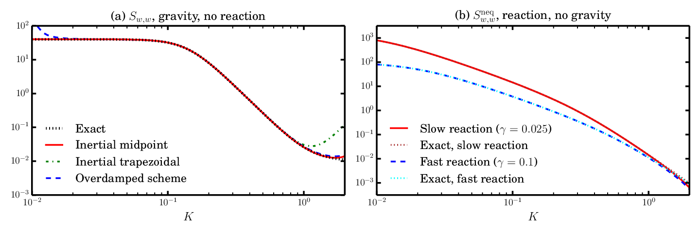
The structure factor can be decomposed into the sum $S_{w,w}=S^{\mathrm{eq}}_{w,w}+S^{\mathrm{neq}}_{w,w}$, where $S^{\mathrm{eq}}_{w,w}$ is the equilibrium structure factor (31) and $S^{\mathrm{neq}}_{w,w}$ is the nonequilibrium enhancement. In the non-reactive case with no gravity, the nonequilibrium enhancement exhibits a $k^{-4}$ power law in the entire range of wavenumbers $k$,

However, the power law is suppressed at small $k$ by gravity [27] or reaction [12].

For the non-reactive case with gravity, we compare $S_{w,w}$ obtained from the three schemes with the exact result in Fig. 2 (a). A power-law spectrum $S_{w,w}\sim k^{-4}$ develops for intermediate wavenumbers $k$. At small wavenumbers, $S_{w,w}$ becomes constant due to gravity. At large wavenumbers, the $k^{-4}$ decay in the nonequilibrium part is hidden due to the flat equilibrium structure factor $S^{\mathrm{eq}}_{w,w}$. Our numerical scheme reproduces $S_{w,w}$ accurately for all but the largest $k$ values, whereas both earlier schemes exhibit significant deviations at either large or small $k$ values. Significant deviations of the previous inertial scheme at large $k$ are due to temporal integration errors in the nonequilibrium part $S^{\mathrm{neq}}_{w,w}$, as can be seen more clearly by examining the cross-correlation between fluctuations of $w$ and $v$ (not shown). The divergence of $S_{w,w}$ for the overdamped scheme at small $k$ demonstrates that the overdamped limit does not apply for sufficiently small $k$ with gravity. Thus, our new scheme combines the favorable features of our previous trapezoidal inertial scheme (correct behavior for small $k$ with gravity) and the overdamped scheme (correct behavior for large $k$).

In Fig. 2 (b), we show the nonequilibrium enhancement $S^{\mathrm{neq}}_{w,w}$ in the structure factor for the reactive case with no gravity. We obtain the exact $S^{\mathrm{neq}}_{w,w}$ by analyzing (53) without the stochastic mass fluxes and with deterministic reaction (see also Eq. (58) in [22] or Eq. (44) in [23]),

References

- [1] A. Vailati and M. Giglio. Giant fluctuations in a free diffusion process. Nature, 390:262–265, 1997.
- [2] L. Lemaigre, M.A. Budroni, L.A. Riolfo, P. Grosfils, and A. De Wit. Asymmetric Rayleigh–Taylor and double-diffusive fingers in reactive systems. Phys. Fluids, 25:014103, 2013.
- [3] A. Donev, A. Nonaka, A.K. Bhattacharjee, A.L. Garcia, and J.B. Bell. Low Mach number fluctuating hydrodynamics of multispecies liquid mixtures. Phys. Fluids, 27:037103, 2015.
- [4] C. Kim, A. Nonaka, J.B. Bell, A.L. Garcia, and A. Donev. Stochastic simulation of reaction-diffusion systems: A fluctuating-hydrodynamics approach. J. Chem. Phys., 146:124110, 2017.
- [5] A. Donev, C.-Y. Yang, and C. Kim. Efficient reactive Brownian dynamics. J. Chem. Phys., 148:034103, 2018.
- [6] N.G. Van Kampen. Stochastic Processes in Physics and Chemistry. North-Holland, Amsterdam, 1983.
- [7] L.D. Landau and E.M. Lifshitz. Fluid Mechanics, chapter XVII, pages 523–529. Pergamon Press, first English edition, 1959. Volume 6 of Course of Theoretical Physics.
- [8] J.M. Ortiz de Zárate and J.V. Sengers. Hydrodynamic Fluctuations in Fluids and Fluid Mixtures. Elsevier, 2006.
- [9] G.A. Bird. Molecular Gas Dynamics and the Direct Simulation of Gas Flows. Clarendon Press, 2nd edition, 1994.
- [10] M. Malek Mansour and F. Baras. Microscopic simulation of chemical systems. Physica A, 188:253–276, 1992.
- [11] F. Baras and M. Malek Mansour. Microscopic simulation of chemical instabilities. Adv. Chem. Phys., 100:393–474, 1997.
- [12] A.K. Bhattacharjee, K. Balakrishnan, A.L. Garcia, J.B. Bell, and A. Donev. Fluctuating hydrodynamics of multi-species reactive mixtures. J. Chem. Phys., 142:224107, 2015.
- [13] C.W. Gardiner. Handbook of Stochastic Methods. Springer-Verlag, 2nd edition, 1985.
- [14] F. Baras and M. Malek Mansour. Reaction-diffusion master equation: A comparison with microscopic simulations. Phys. Rev. E, 54:6139–6148, 1996.
- [15] G. Nicolis and I. Prigogine. Self-Organization in Nonequilibrium Systems. Wiley-Interscience, 1977.
- [16] P. Dziekan, L. Signon, B. Nowakowski, and A. Lemarchand. Reaction-diffusion approach to prevertebrae formation: Effect of a local source of morphogen. J. Chem. Phys., 139:114107, 2013.
- [17] I. Pagonabarraga, A. Pérez-Madrid, and J.M. Rubí. Fluctuating hydrodynamics approach to chemical reactions. Physica A, 237:205–219, 1997.
- [18] D. Bedeaux, I. Pagonabarraga, J.M. Ortiz de Zárate, J.V. Sengers, and S. Kjelstrup. Mesoscopic non-equilibrium thermodynamics of non-isothermal reaction-diffusion. Phys. Chem. Chem. Phys., 12:12780–12793, 2010.
- [19] J. Keizer. Statistical Thermodynamics of Nonequilibrium Processes. Springer-Verlag, New York, 1987.
- [20] D.T. Gillespie, A. Hellander, and L.R. Petzold. Perspective: Stochastic algorithms for chemical kinetics. J. Chem. Phys., 138:170901, 2013.
- [21] R. Erban, J. Chapman, and P. Maini. A practical guide to stochastic simulations of reaction-diffusion processes. ArXiv e-prints, 2007.
- [22] J.M. Ortiz de Zárate, J.V. Sengers, D. Bedeaux, and S. Kjelstrup. Concentration fluctuations in nonisothermal reaction-diffusion systems. J. Chem. Phys., 127:034501, 2007.
- [23] D. Bedeaux, J.M. Ortiz de Zárate, I. Pagonabarraga, J.V. Sengers, and S. Kjelstrup. Concentration fluctuations in non-isothermal reaction-diffusion systems. II. The nonlinear case. J. Chem. Phys., 135:124516, 2011.
- [24] A. Donev, E. Vanden-Eijnden, A. Garcia, and J. Bell. On the accuracy of finite-volume schemes for fluctuating hydrodynamics. Comm. App. Math. Comp. Sci., 5:149–197, 2010.
- [25] K. Balakrishnan, A.L. Garcia, A. Donev, and J.B. Bell. Fluctuating hydrodynamics of multispecies nonreactive mixtures. Phys. Rev. E, 89:013017, 2014.
- [26] A. Nonaka, Y. Sun, J.B. Bell, and A. Donev. Low Mach number fluctuating hydrodynamics of binary liquid mixtures. Comm. App. Math. Comp. Sci., 10:163–204, 2015.
- [27] A. Donev, A. Nonaka, Y. Sun, T.G. Fai, A.L. Garcia, and J.B. Bell. Low Mach number fluctuating hydrodynamics of diffusively mixing fluids. Comm. App. Math. Comp. Sci., 9:47–105, 2014.
- [28] M. Cai, A. Nonaka, J.B. Bell, B.E. Griffith, and A. Donev. Efficient variable-coefficient finite-volume Stokes solvers. Commun. Comput. Phys., 16:1263–1297, 2014.
- [29] Y. Hu, T. Li, and B. Min. A weak second order tau-leaping method for chemical kinetic systems. J. Chem. Phys., 135:024113, 2011.
- [30] D.T. Gillespie. Approximate accelerated stochastic simulation of chemically reacting systems. J. Chem. Phys., 115:1716–1733, 2001.
- [31] A.J. Chorin and J.E. Marsden. A Mathematical Introduction to Fluid Mechanics, volume 3. Springer, 1990.
- [32] M.R. Marcelin. Sur la mécanique des phénomènes irréversibles. Comptes rendus hebdomadaires des séances de l’Académie des sciences, tome 151:1052–1055, 1910.
- [33] In a reaction-diffusion setting, this means that diffusion dominates on the length scale of a reactive cell. Equivalently, for typical diffusion coefficient and linearized reaction rate , the penetration depth is significantly larger than , which is itself much larger than molecular scales. In this reaction-limited case, the validity of the mesoscopic description of reactions is guaranteed. On the other hand, for a diffusion-limited system, where becomes comparable to molecular scales, the validity of the CME remains to be investigated [5].
- [34] D. Kelly and E. Vanden-Eijnden. Fluctuations in the heterogeneous multiscale methods for fast-slow systems. Res. Math. Sci., 4:23, 2017.
- [35] S. Delong, Y. Sun, B.E. Griffith, E. Vanden-Eijnden, and A. Donev. Multiscale temporal integrators for fluctuating hydrodynamics. Phys. Rev. E, 90:063312, 2014.
- [36] F.B. Usabiaga, J.B. Bell, R. Delgado-Buscalioni, A. Donev, T.G. Fai, B.E. Griffith, and C.S. Peskin. Staggered schemes for fluctuating hydrodynamics. Multiscale Model. Simul., 10:1369–1408, 2012.
- [37] J.B. Bell, C.N. Dawson, and G.R. Shubin. An unsplit, higher order Godunov method for scalar conservation laws in multiple dimensions. J. Comp. Phys., 74:1–24, 1988.
- [38] A. Nonaka, S. May, A.S. Almgren, and J.B. Bell. A three-dimensional, unsplit Godunov method for scalar conservation law. SIAM J. Sci. Comput., 33:2039–2062, 2011.
- [39] D.F. Anderson and J.C. Mattingly. A weak trapezoidal method for a class of stochastic differential equations. Commun. Math. Sci., 9:301–318, 2011.
- [40] S. Delong, B.E. Griffith, E. Vanden-Eijnden, and A. Donev. Temporal integrators for fluctuating hydrodynamics. Phys. Rev. E, 87:033302, 2013.
- [41] A. Venâncio and J.A. Teixeira. Characterization of sugar diffusion coefficients in alginate membranes. Biotechnol. Tech., 11:183–185, 1997.
- [42] J.F. Tilley and R. Mills. Relations between mutual and intradiffusion coefficients in aqueous sucrose solutions. J. Phys. Chem., 71:2756–2757, 1967.
- [43] K. Krynicki, C.D. Green, and D.W. Sawyer. Pressure and temperature dependence of self-diffusion in water. Faraday Discuss. Chem. Soc., 66:199–208, 1978.
- [44] X. Liu, A. Bardow, and T.J.H. Vlugt. Multicomponent Maxwell–Stefan diffusivities at infinite dilution. Ind. Eng. Chem. Res., 50:4776–4782, 2011.
- [45] R.N. Goldberg, Y.B. Tewari, and J.C. Ahluwalia. Thermodynamics of the hydrolysis of sucrose. J. Biol. Chem., 264:9901–9904, 1989.
- [46] R. Wolfenden and Y. Yuan. Rates of spontaneous cleavage of glucose, fructose, sucrose, and trehalose in water, and the catalytic proficiencies of invertase and trehalas. J. Am. Chem. Soc., 130:7548–7549, 2008.
- [47] J.M. Ortiz de Zárate, T.R. Kirkpatrick, and J.V. Sengers. Non-equilibrium concentration fluctuations in binary liquids with realistic boundary conditions. Eur. Phys. J. E, 38:99, 2015.
- [48] C. Almarcha, P.M.J. Trevelyan, P. Grosfils, and A. De Wit. Thermal effects on the diffusive layer convection instability of an exothermic acid-base reaction front. Phys. Rev. E, 88:033009, 2013.
- [49] R. Erban and S.J. Chapman. Stochastic modeling of reaction-diffusion processes: Algorithms for bimolecular reactions. Phys. Biol., 6:046001, 2009.
- [50] M.J. Esplandiu, A.A. Farniya, and D. Reguera. Key parameters controlling the performance of catalytic motors. J. Chem. Phys., 144:124702, 2016.
- [51] M.B. Andersen, K.M. Wang, J. Schiffbauer, and A. Mani. Confinement effects on electroconvective instability. Electrophoresis, 38:702–711, 2017.
- [52] J.-P. Péraud, A. Nonaka, A. Chaudhri, J.B. Bell, A. Donev, and A.L. Garica. Low Mach number fluctuating hydrodynamics for electrolytes. Phys. Rev. Fluids, 1:074103, 2016.
- [53] B.E. Griffith and C.S. Peskin. Electrophysiology. Commun. Pure Appl. Math., 66:1837–1913, 2013.
- [54] J.L. Moran and J.D. Posner. Electrokinetic locomotion due to reaction-induced charge auto-electrophoresis. J. Fluid Mech., 680:31–66, 2011.
- [55] J.L. Moran and J.D.Posner. Phoretic self-propulsion. Annu. Rev. Fluid Mech., 49:511–540, 2017.