Soft-gluon corrections in top-quark production
Nikolaos Kidonakis
Department of Physics, Kennesaw State University,
Kennesaw, GA 30144, USA
Abstract
I review calculations of soft-gluon corrections for top-quark production in hadron collisions. I describe theoretical formalisms for their resummation and for finite-order expansions. I show that soft-gluon corrections are dominant for a large number of top-quark processes. I discuss top-antitop pair production as well as single-top production, including total cross sections and differential distributions, and compare with data from the LHC and the Tevatron. I also discuss top-quark production in association with charged Higgs bosons, bosons, and other particles in models of new physics.
1 Introduction
Top-quark physics is a central element in the exploration of particle physics at hadron colliders. The top quark occupies a special place as the heaviest elementary particle to have been found, and the only quark that decays before it can hadronize. It was discovered via the top-antitop pair production process in proton-antiproton collisions at the Fermilab Tevatron by the CDF and D0 Collaborations in 1995 [1, 2]. Single-top production events were also first seen at the Tevatron [3, 4]. The top quark was later rediscovered at the LHC in [5, 6] processes. The LHC now serves as a top-quark factory.
In this paper I review top-quark production in hadron colliders, focusing on higher-order corrections from soft-gluon resummation. There is a very long history of resummations for top-pair production, Refs. [7-67], for single-top production, Refs. [68-77], as well as for top-quark production in models of new physics, Refs. [78-84].
Next-to-leading order (NLO) [85, 86, 87] and next-to-next-to-leading order (NNLO) [88, 89, 90, 91] corrections have been available for top-pair production for some time. For single-top production, NLO corrections for the and channels [92] and for production [93] are also known, while NNLO corrections [94, 95, 96] have been calculated for the -channel. Higher-order soft-gluon corrections can further improve the NLO and NNLO results.
In Section 2, I begin with a brief history of soft-gluon resummation, followed by a general discussion of higher-order soft-gluon corrections, factorization, renormalization-group evolution, resummation, and expansions at NLO, NNLO, and next-to-next-to-next-to-leading order (N3LO).
In Section 3, I continue with a review of the cusp anomalous dimension and of soft anomalous dimension matrices for production through two loops. In Section 4, I provide results for the total cross sections, the top-quark transverse momentum, , distributions, and the top-quark rapidity distributions at the LHC and the Tevatron, as well as the forward-backward asymmetry at the Tevatron.
In Section 5, I discuss single-top production, including -channel and -channel production, and production, and I present total cross sections and top-quark and rapidity distributions. In Section 6, I discuss top-quark production in association with a charged Higgs boson, and in association with gauge bosons via anomalous couplings in new-physics models. I conclude with a summary in Section 7.
2 Soft-gluon corrections
Soft-gluon corrections arise from the emission of low-energy gluons, and they result from incomplete cancellations of infrared divergences between virtual diagrams and diagrams with real emission.
These corrections appear in the perturbative series as plus distributions involving logarithms of a variable that measures the kinematical distance from threshold. For the th-order perturbative corrections, the leading logarithms are those with the highest power, ; the next-to-leading logarithms have a power of ; etc. The effects of soft-gluon corrections are particularly relevant near partonic threshold. At partonic threshold there is no energy for additional radiation, but the top quark may have non-zero momentum and is not restricted to be produced at rest. Thus, partonic threshold is a more general concept than production or absolute threshold, where the top quark is produced at rest.
For top-antitop production, several threshold variables have been used for resummation. In single-particle-inclusive (1PI) kinematics, the partonic threshold variable is where , , and are the standard kinematical variables and the sum is over the masses squared of all particles in the scattering. At partonic threshold, . In pair-invariant-mass (PIM) kinematics, the partonic threshold variable is , where is the invariant mass of the top-antitop pair; at partonic threshold . In resummation using absolute threshold - a special limiting case of partonic threshold as we discussed above - the threshold variable is , where is the top-quark mass; at absolute threshold, .
Formalisms that use partonic threshold in 1PI or PIM kinematics involve a general resummation for double-differential distributions, from which single distributions or total cross sections can be derived by appropriate integrations. Formalisms that use absolute threshold are limited only to total cross sections.
Similarly, 1PI kinematics have been used in resummations for single-top production using the threshold variable .
Soft-gluon corrections are dominant near threshold and usually even far from threshold. These corrections can be formally resummed to all orders in perturbative QCD. This resummation, i.e. exponentiation, follows from the factorization properties of the cross section and from the renormalization-group evolution of the functions in the factorized form.
Leading-logarithm (LL) resummations and their finite-order expansions for top-antitop pair production were developed and used in various formalisms in Refs. [7, 8, 9, 10, 11, 12, 15, 18]. Next-to-leading-logarithm (NLL) resummations and their expansions were developed and used for double-differential cross sections in Refs. [13, 17, 20, 21, 22, 23, 24, 25] using partonic threshold, and in Refs. [19, 26] for only total cross sections. Corrections beyond NLL in expansions were calculated in Refs. [23, 25, 27, 28, 30, 31, 33]. Next-to-next-to-leading-logarithm (NNLL) resummations and expansions were developed in Refs. [35, 36, 37, 38, 39, 40, 41, 45, 48, 49, 50, 51].
Leading logarithms can be resummed in terms of universal terms for the emission of collinear and soft gluons; these universal terms only depend on the identity of the incoming and outgoing partons. However, at NLL accuracy and beyond [13, 17] resummation involves the process-dependent color exchange in the hard-scattering process.
More explicitly, in 1PI kinematics the soft-gluon terms are of the form where for the th-order perturbative corrections, and is the kinematical distance from partonic threshold described above. We define
| (1) |
where is a small parameter that separates the hard-gluon, , and soft-gluon, , regions.
In PIM kinematics the soft-gluon terms are of the form , where again for the th-order perturbative corrections, and is the kinematical distance from partonic threshold described above. We define
| (2) |
where, again, is a small parameter that separates the hard-gluon, , and soft-gluon, , regions.
2.1 Factorization and Resummation
We consider top-quark production in proton-proton collisions at the LHC,
| (3) |
and proton-antiproton collisions at the Tevatron
| (4) |
where denotes the observed top quark, with all additional final-state particles. The partonic processes involved are of the form
| (5) |
where and are partons (quarks and/or gluons). We define the usual kinematical variables , , . We also define, as before, the 1PI partonic threshold variable .
The factorized form of the (differential) cross section may be written in 1PI kinematics as
| (6) |
where is the factorization scale and is the renormalization scale. A similar expression applies to PIM kinematics. The parton distribution functions (pdf), , describe the fraction of the proton momentum carried by the partons, with and the momentum fractions of partons and in protons and respectively.
Soft-gluon corrections in the partonic cross section, , contribute terms with plus distributions of logarithms of or , defined via their integral with the pdf. In 1PI kinematics
| (7) | |||||
while in PIM kinematics
| (8) | |||||
These are equivalent definitions to Eqs. (1) and (2), respectively.
The resummation of soft-gluon contributions results from the factorization properties of the cross section in moment space. Moments of the partonic cross section are defined by in 1PI kinematics, and in PIM kinematics. Logarithms of or transform in moment space into logarithms of , which exponentiate.
We write the moment-space partonic cross section, in dimensions, in factorized form, as
| (9) |
with .
The is the hard-scattering function that does not depend on , and it describes contributions from the amplitude and the complex conjugate of the amplitude for the process. The soft-gluon function describes the coupling of soft gluons to the partons in the scattering. The analytical form of and depends on the process, and in general both functions are matrices in color space in the partonic scattering. The and are jet functions that describe universal soft and collinear emission from incoming and outgoing massless partons.
The -dependence of the soft matrix can be resummed via renormalization group evolution [13, 17]. We have
| (11) |
where is the unrenormalized quantity and is a matrix of renormalization constants. Thus satisfies the renormalization group equation
| (12) |
where , and is the QCD beta function
| (13) |
where , , with the number of colors, and is the number of light quark flavors ( for top production).
The soft anomalous dimension, , controls the evolution of the soft function . We determine from the coefficients of the ultraviolet poles of eikonal diagrams. In dimensional regularization has poles, and is given in terms of the residue of [13, 17]. In general, is a matrix in color space as well as a function of the kinematic variables , , .
The resummed cross section in moment space is derived from the renormalization-group evolution of the functions in the factorized cross section, and can be written as
where the trace is taken of the product of the color-space hard and soft matrices, and the exponents of .
The collinear-gluon and soft-gluon contributions from the initial-state partons are resummed in the first exponential in Eq. (), with exponent
| (15) |
Here we have defined and . The perturbative series for is written as , with [97] where for a quark or antiquark, while for a gluon; and [98] where [99], with . Also the perturbative series for is written as , with in Feynman gauge.
The collinear-gluon and soft-gluon contributions from final-state massless quarks and/or gluons are resummed in the second exponential, with exponent
| (16) | |||||
where we have defined . The perturbative series for is written as , with for a quark or antiquark, and for a gluon [97, 98]. Note that this exponent is not needed in or production but it is used in -channel and -channel single-top production.
The factorization-scale dependence in the third exponential is given in moment space by the anomalous dimension of , which is , where with the Euler constant, and with , .
The perturbative series for the hard function and the soft function are written as and , respectively, where denotes the power of in the leading-order (LO) cross section. The LO cross section for each partonic process is given by the trace of the product of the lowest-order hard and soft matrices: .
Noncollinear soft-gluon emission is described by the soft anomalous dimension , with perturbative expansion
| (17) |
The first term in the series, , requires one-loop calculations and is needed for NLL resummation, while requires two-loop calculations and is needed for NNLL resummation.
2.2 Methods and prescriptions
There are numerous and very substantive differences between the various resummation approaches in the literature, which have been detailed previously in Refs. [53, 60]. Some formalisms have been developed to do the resummation only for the total cross section while others are for the double-differential cross section; some formalisms use moment-space perturbative QCD while others use Soft-Collinear Effective Theory (SCET). The treatment of subleading logarithms in different formalisms and the approach to deal with infrared divergences via prescriptions or finite-order expansions lead to large differences in numerical results.
The more general double-differential approach to resummation can be expressed in 1PI kinematics for the differential cross section in top-quark transverse momentum and rapidity, , where the soft limit is , or in PIM kinematics for the differential cross section in top-pair invariant mass and scattering angle, , where the soft limit is . Such double-differential approaches have been developed in moment-space in QCD, Refs. [13, 17, 20, 22, 23, 24, 25, 27, 28, 30, 49, 60, 61, 64], as well as in SCET, Refs. [40, 41, 45, 50]. Double-differential distributions, single-differential distributions, and total cross sections can all be derived via the above formalisms. Resummations that are developed for the total cross section only refer to production (or absolute) threshold and resum logarithms of , Refs. [19, 31, 38, 47, 48, 55]. The soft limit here is the production threshold limit (where the top quark velocities are zero), which is a special case of the more general partonic threshold.
The resummed cross section encounters infrared divergences that require a prescription to be dealt with, and the choice of prescription is to an extent arbitrary. Moreover, the numerical results depend greatly on the prescription, and differences between prescriptions are typically larger than corrections beyond NNLO. In order to avoid arbitrary prescription dependence, an excellent approach is to expand the resummed cross section to a fixed order, usually NNLO or N3LO; this gives better control of subleading terms.
The relative size of soft-gluon corrections has been argued about since the 1990’s. The LL results in Refs. [7, 8, 9] and [10, 12, 18] argued for large effects. The LL results in [11, 15], using the minimal prescription, argued for tiny corrections, one or two orders of magnitude smaller. Similarly at NLL, the results in Ref. [19], which were based on the minimal prescription, were much smaller than the results in Refs. [23, 24], which were based on Refs. [13, 17, 20] and used fixed-order expansions. In Ref. [55] the predictions with minimal prescription are small for both Tevatron and LHC energies and they account for only a very small fraction of the NNLO corrections. In contrast the predictions in Ref. [27, 33] and the NNLL predictions in Refs. [49, 51], using fixed-order expansions, predicted the NNLO corrections, which are large, extremely well.
2.3 NLO, NNLO, and N3LO expansions
Here we present expansions of the resummed cross section through N3LO. We use the notation for the logarithmic plus distributions of Eqs. (1) and (2). We give results for 1PI kinematics first.
The NLO soft-gluon corrections from the expansion of the resummed cross section are given by
| (18) |
where is the LO term. The LL coefficient is
| (19) |
and it multiplies . The NLL terms are in general not all proportional to . The coefficient is defined by , with denoting the terms involving logarithms of the scale, and
| (20) | |||||
where stands for or , while is defined by
| (21) |
The NNLO soft-gluon corrections from the expansion of the resummed cross section are
| (22) | |||||
where for brevity we do not show further subleading terms.
The N3LO soft-gluon corrections from the expansion of the resummed cross section are
| (23) | |||||
where, again for brevity, we do not show further subleading terms.
Results for PIM kinematics are analogous: we replace by and drop terms involving the variables in the above expressions.
3 Soft anomalous dimensions in top-pair production
3.1 Cusp anomalous dimension

The Feynman rules for diagrams with soft gluon emission simplify in the eikonal approximation (see Fig. 1), as
| (24) |
where is a Dirac spinor, are the generators of SU(3), and .
We begin with the massive cusp anomalous dimension [35], which is the simplest soft anomalous dimension and an essential component of calculations for top-quark production. Calculations can be performed in momentum space and in Feynman gauge, although other choices are possible.

The one-loop diagrams for the cusp anomalous dimension, with eikonal lines representing the top and the antitop quarks, are shown in Fig. 2. The left graph (a) is the one-loop vertex correction, while the graph on the right (b) shows the one-loop top and antitop self-energy diagrams.
The one-loop cusp anomalous dimension, , is found from the coefficient of the ultraviolet pole of the one-loop diagrams [35]:
| (25) |
where, as before, .
In terms of the cusp angle [100], where , or , we can rewrite the one-loop expression as
| (26) |


At two loops, the vertex-correction graphs for the cusp anomalous dimension are shown in Fig. 3 while the top-quark self-energy graphs are shown in Fig. 4. The grey blobs in the diagrams represent quark, gluon, and ghost loops.
With the inclusion of counterterms and after multiplying with the relevant color factors, the two-loop cusp anomalous dimension, as determined from the ultraviolet poles, is [35]:
| (27) | |||||
where .
An excellent approximation to the complete two-loop result that is valid for all is given by [35]:
| (28) |
3.2 Soft anomalous dimension matrices for production


The top-antitop pair production partonic processes at lowest order are
| (30) |
and
| (31) |
The diagrams for these processes are shown in Fig. 5. We define , , and .
Next, we present the one-loop and two-loop results for the soft anomalous matrices for these partonic processes. The soft anomalous dimension matrix for in a color tensor basis of -channel singlet and octet exchange,
| (32) |
can be written as
The soft anomalous dimension matrix for in a color tensor basis
| (39) |
where and are the totally symmetric and antisymmetric tensors, is
4 Top-antitop pair production
4.1 Total cross sections for production
| Collider Energy | Cross section scale pdf |
|---|---|
| 1.8 TeV | |
| 1.96 TeV | |
| 5.02 TeV | |
| 7 TeV | |
| 8 TeV | |
| 13 TeV | |
| 14 TeV |
We begin our presentation of numerical results with the total cross section for top-antitop pair production. The total hadronic cross section is calculated by integrating over the convolution of the double-differential partonic cross section with the parton distribution functions .
We denote the NLO soft-gluon corrections from the expansion of the NNLL resummed cross section as approximate NLO (aNLO) corrections. Similarly the NNLO soft-gluon corrections are denoted as approximate NNLO (aNNLO) corrections, and the N3LO soft-gluon corrections are denoted as approximate N3LO (aN3LO) corrections. The aNLO and aNNLO corrections are extremely good approximations to the exact NLO and NNLO results, respectively, for total cross sections as well as top-quark differential distributions at all Tevatron and LHC energies (see e.g. the discussion in Ref. [60]). The best aN3LO prediction is given by the sum of the NNLO cross section and the aN3LO soft-gluon corrections.

A comparison of various approximate predictions using higher-order soft-gluon corrections, all made before the exact NNLO cross section was known, is shown in Fig. 6, all with the same choice of parameters and MSTW2008 [103] pdf, at 1.96 TeV Tevatron energy and at 7, 8, and 14 TeV LHC energies. Moreover, exact NLO and NNLO results for the total cross sections are also shown on the plot. We observe the success or lack thereof of the various predictions in predicting the exact NNLO result.
Ref. [49] uses the QCD moment-space resummation formalism for the double-differential cross section. Ref. [47] uses QCD moment-space resummation with absolute threshold for the total-only cross section. Ref. [44] uses the SCET resummation formalism for the double-differential cross section, while Ref. [54] uses SCET resummation with absolute threshold for the total-only cross section. Lastly, Ref. [55] uses QCD moment-space resummation with absolute threshold for the total-only cross section.
The result in Ref. [49] is very close to the exact NNLO [88] result: the central values and the scale uncertainty are nearly identical, for all collider energies, with less than 1% difference between approximate and exact cross sections. This was expected from the comparison of approximate NNLO results in different kinematics in Ref. [27] (see also the discussions in [49] and [60]).

In Fig. 7 we display theoretical predictions at aN3LO[61] for the total cross section as a function of top-quark mass at the LHC and the Tevatron. We use MMHT2014 [104] NNLO pdf but note that the results with CT14[105] and NNPDF [106] pdf are very similar. We compare the aN3LO results with data from the LHC at 5.02 TeV [107], 7 TeV [108, 109], 8 TeV [110, 109], and 13 TeV [111, 112], and from the Tevatron at 1.8 TeV [113, 114] and 1.96 TeV [115]. We find superb agreement between the theoretical predictions and the data.
4.2 Top-quark and rapidity distributions in production
We continue with top quark differential distributions in production. We present theoretical results for the top-quark transverse momentum and rapidity distributions at Tevatron and LHC energies.

The aN3LO top-quark distributions [64], with scales , , and , and GeV, are displayed in Fig. 8 at 7, 8, 13, and 14 TeV LHC energies.


The left plot in Fig. 9 shows the aN3LO top-quark normalized distribution, , at the LHC compared to CMS [116] data at 13 TeV energy. Two different choices of scale are used, and , where . There is excellent agreement with data. In the right plot of Fig. 9, the aN3LO top-quark normalized distribution at 8 TeV LHC energy with scale and is compared to ATLAS [117] data, again with excellent agreement. The high- region is highlighted in the inset plots.


Figure 10 shows the aN3LO top-quark normalized distribution at the LHC compared to CMS [118] data at 8 TeV energy. There is excellent agreement with data in both the dilepton and lepton+jets channels.


Figure 11 shows the aN3LO boosted-top quark distribution at the LHC compared to ATLAS [119] and CMS [120] data at 8 TeV energy. There is excellent agreement with the data.


The aN3LO top-quark normalized distribution at 7 TeV LHC energy is shown in Fig. 12 and compared with CMS [121] data in the dilepton and lepton+jets channels. We note the excellent agreement of theory with data.


In the left plot of Fig. 13, the aN3LO top-quark normalized distribution at 7 TeV LHC energy is compared to ATLAS [122] data. The right plot of Fig. 13 displays the aN3LO top quark distribution at 1.96 TeV Tevatron energy. Excellent agreement of the aN3LO results with D0 data [123] can be seen, including the high- region shown in the inset.

The aN3LO top-quark rapidity distributions at 7, 8, 13, and 14 TeV LHC energies are displayed in Fig. 14 with scale choices , , and .


The aN3LO top-quark normalized rapidity distribution, , at 13 TeV LHC energy is shown in the left plot of Fig. 15 and compared with CMS [116] data. In the right plot of Fig. 15, the aN3LO top-quark normalized absolute value rapidity distribution at 8 TeV LHC energy is compared to ATLAS [117] data. We find excellent agreement between theory and data in both cases.


The aN3LO top-quark normalized rapidity distribution at 8 TeV LHC energy is shown in Fig. 16 and compared with CMS [118] dilepton and lepton+jets data, again with excellent agreement.


The aN3LO top-quark normalized rapidity distribution at 7 TeV LHC energy is shown in Fig. 17 and compared with CMS [121] dilepton and lepton+jets data. We again note the excellent agreement between theory and data.


4.3 Top-quark forward-backward asymmetry
The top-quark forward-backward asymmetry is defined by
| (46) |
The asymmetry is very significant at the Tevatron. In addition to QCD corrections, electroweak corrections are important for this asymmetry [124, 125, 126, 127] (see also Ref. [128] for rapidity distributions at the LHC). The theoretical result at aN3LO and including electroweak corrections for 1.96 TeV Tevatron energy is [65] which is in agreement with the CDF and D0 combination [129] of . The aN3LO differential is plotted in the right plot of Fig. 18 and compared with D0 [130] and CDF [131] data.
5 Single-top production
| Collider | -channel | -channel | -channel | -channel | -channel | -channel | |
| Energy | and | and | |||||
| 1.96 TeV | 1.088 | 1.088 | 2.176 | 0.52 | 0.52 | 1.04 | 0.102 |
| 7 TeV | 43.9 | 23.7 | 67.6 | 3.21 | 1.56 | 4.77 | 8.5 |
| 8 TeV | 57.5 | 31.7 | 89.2 | 3.86 | 1.96 | 5.82 | 12.0 |
| 13 TeV | 139.6 | 84.0 | 223.6 | 7.29 | 4.20 | 11.49 | 38.1 |
| 14 TeV | 158.3 | 96.1 | 254.3 | 7.98 | 4.68 | 12.66 | 44.8 |


Single-top-quark production was first observed at the Tevatron in 2009 [3, 4]. The single-top partonic processes at lowest order are shown in Fig. 19.
The -channel partonic processes are of the form and and are numerically the largest among single-top processes at Tevatron and LHC energies. The -channel partonic processes are of the form and are numerically second largest at the Tevatron and the smallest at the LHC among single-top processes. The associated production proceeds via and is negligible at the Tevatron but second largest numerically among single-top processes at the LHC.
Table 2 summarizes the central values of the cross sections for the various single-top channels at LHC and Tevatron energies.
5.1 -channel production
We start with single-top production in the -channel.
The soft anomalous dimension matrix for -channel single-top production is a matrix, and it has been calculated at one loop in Refs. [68, 73] and at two loops in Ref. [73]. The elements of this matrix are given at one-loop by [68, 73]
At two loops, the first element of this matrix is given by [73]
| (48) |
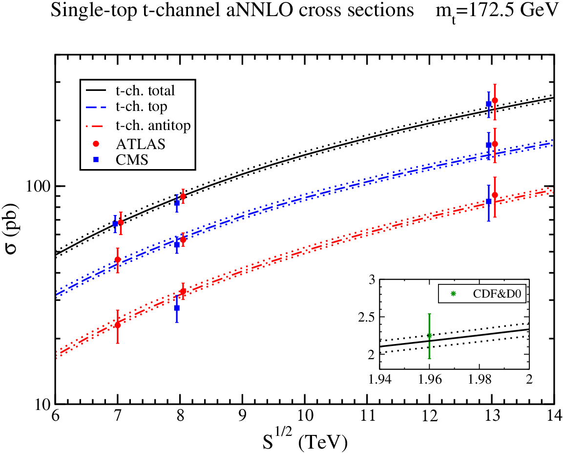
In Figure 20 we plot the aNNLO -channel single-top and single-antitop cross sections, and their sum, with GeV with theoretical uncertainty from scale variation and the pdf error. Excellent agreement is found with D0 and CDF combination [132] at 1.96 TeV energy, and with CMS [133, 135, 138] and ATLAS [134, 136, 137] results at 7, 8, and 13 TeV energies.
The theoretical ratio at 7 TeV compares well with the ATLAS [134] result of . The theoretical ratio at 8 TeV compares well with the ATLAS [136] result of and the CMS [135] result of . The theoretical ratio for the total -channel cross section (8 TeV)/(7 TeV)= compares well with the CMS [135] result of . The theoretical ratio at 13 TeV is in agreement with the ATLAS [137] result of and the CMS result [138] of .


In addition to the total cross section, the top-quark distribution in -channel production is of great interest. Figure 21 shows the top (left) and antitop (right) aNNLO distributions in -channel production at 7 TeV LHC energy together with data from ATLAS [134].


Figure 22 shows the top (left) and antitop (right) aNNLO normalized distributions in -channel production at 8 TeV LHC energy. We find very good agreement between theory and data from ATLAS [136] for both distributions.


The left plot of Fig. 23 shows the top-quark aNNLO normalized distribution in -channel production at 8 TeV LHC energy compared to CMS [139] data. We note the very good agreement between theory and data. The plot on the right of Fig. 23 shows the top plus antitop aNNLO normalized distribution in -channel production at 13 TeV LHC energy compared to CMS [140] data.
5.2 -channel production
We continue with single-top production in the -channel.
The soft anomalous dimension matrix for this process has been calculated at one loop[68, 70] and at two loops[70]. The matrix for -channel single-top production at one loop is [68, 70]
The first element of this matrix at two loops is [70]
| (50) |
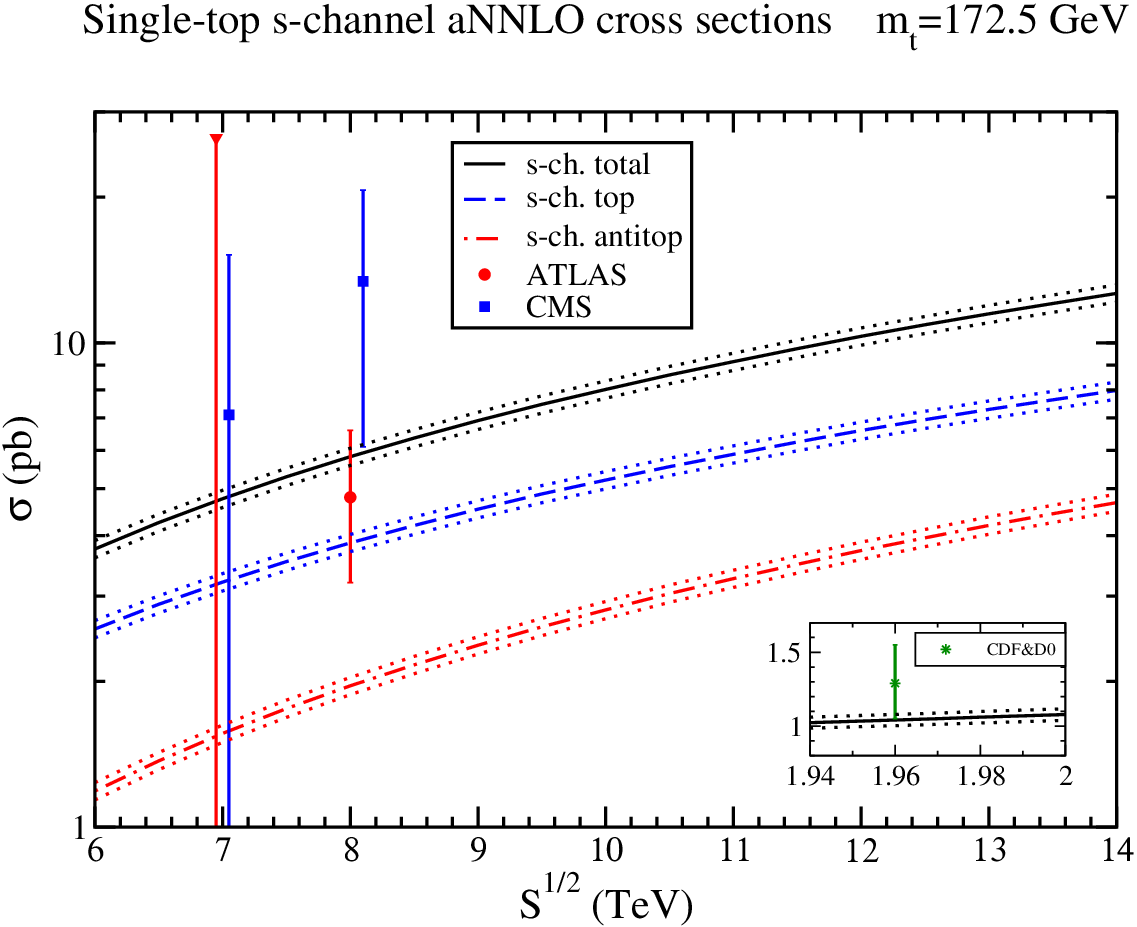
Figure 24 shows the aNNLO cross sections for -channel production with theoretical uncertainty from scale variation and pdf error. Results are shown for single-top production, single-antitop production, and their sum. Excellent agreement is found with D0 and CDF combination [144], CMS [142], and ATLAS [143] results.
5.3 production
We continue with the associated production of a top quark with a boson. The cross section for production is identical to that for .
The soft anomalous dimension for is given at one loop by [68, 71]
| (51) |
and at two loops by [71]
| (52) |

Fig. 25 shows the total aN3LO [77] cross section (sum of and ) as a function of LHC energy. Excellent agreement is found with data from ATLAS [145] and CMS [146] at 7 TeV, an ATLAS/CMS combination at 8 TeV [147], and ATLAS [148] and CMS[149] at 13 TeV.


6 Top-quark production in models of new physics
In addition to the various Standard-Model processes for top-quark production, some of which we studied above, other possibilities include top production in association with particles in models of new physics, or top production via top-quark anomalous couplings. We consider some of these possibilities below.
6.1 Associated production of a top quark with a charged Higgs boson

We first consider the production of a top quark in association with a charged Higgs boson [80, 71, 83]. Charged Higgs bosons appear in the Minimal Supersymmetric Standard Model (MSSM) and other two-Higgs doublet models. The lowest-order diagrams for this process are shown in Fig. 27. The soft anomalous dimension for this process is the same as for production.


The left plot in Fig. 28 shows the aNNLO cross section for production in the MSSM, with , at LHC energies as a function of charged-Higgs mass. The aNNLO corrections increase the NLO cross section significantly, with the particular value of the increase depending on the charged-Higgs mass. The plot on the right in Fig. 28 shows the aNNLO normalized top-quark distributions in production for a charged-Higgs mass of 300 GeV.


6.2 Associated production of a top quark with a boson via anomalous couplings

An interesting process that involves top-quark anomalous couplings is the associated production of a top quark with a boson. While production can proceed via Standard Model processes involving an additional quark in the final state, it is possible to produce a final state without any other particles in models with anomalous couplings [79, 84]. The lowest-order diagrams are shown in Fig. 30.
An effective Lagrangian that includes an anomalous coupling of a pair to a boson is
| (53) |
where is the anomalous -- coupling with an up or charm quark, is the -boson field tensor, with Dirac matrices , and is an effective scale which we take to be the top-quark mass.
Soft-gluon corrections have been calculated at aNNLO in Ref. [84]. These soft corrections are important, and in fact at NLO they approximate the exact NLO [150] results remarkably well for both and . The aNNLO corrections provide additional enhancements.


The left plot of Fig. 31 shows the aNNLO total cross sections for with at 7, 8, 13, and 14 TeV LHC energies as functions of the top-quark mass, with scales set equal to the top-quark mass. The inset plot shows the aNNLO/NLO -factors at the various LHC energies. The aNNLO corrections increase the NLO result significantly at all LHC energies.
The right plot of Fig. 31 shows the aNNLO top-quark distributions, , at 7, 8, 13, and 14 TeV LHC energies with GeV and .
6.3 Other top-quark production processes via anomalous couplings
In addition to production discussed in the previous subsection, top quarks can also be produced in association with or bosons [151] (see Ref. [152] for models of such particles). Soft-gluon corrections are significant for such processes [151].
The production of top quarks with photons, , via anomalous -- couplings, with an up or charm quark, at Tevatron energy was studied in Ref. [79]. The soft-gluon corrections were found to be significant. The corrections are also large at LHC energies [153].
The process in electron-proton collisions via anomalous -- coupling was studied in Ref. [78]. The processes , with an up or charm quark, via anomalous -- and -- couplings, were studied in Ref. [79]. The soft-gluon corrections were found to be important.
Same-sign top-quark production, , with an up or charm quark, via anomalous -- and -- couplings, was studied in Ref. [79]. Numerical results were given for Tevatron energy [79].
The process via anomalous -- couplings was studied in detail in Ref. [81]. The soft-gluon corrections were found to be substantial at LHC energies.
7 Summary
In this review, I have discussed soft-gluon corrections for top-quark production in hadronic collisions. I have presented the resummation of soft-gluon contributions in various top-quark processes through NNLL accuracy via two-loop calculations of soft anomalous dimension matrices.
N3LO approximate results with soft-gluon corrections for the production cross section, and the top-quark differential distributions in transverse momentum and rapidity, are in excellent agreement with data from the LHC and the Tevatron. Single-top cross sections and differential distributions have been presented in the -channel and -channel, and in production, and they are also in excellent agreement with collider data.
Top-quark production in association with charged-Higgs bosons or with anomalous couplings in models of new physics has also been discussed. Soft-gluon corrections are very significant for all top-quark production processes, and they reduce the theoretical errors.
Acknowledgments
This material is based upon work supported by the National Science Foundation under Grant No. PHY 1519606.
References
- [1] CDF Collab., Phys. Rev. Lett. 74, 2626 (1995) [hep-ex/9503002].
- [2] D0 Collab., Phys. Rev. Lett. 74, 2632 (1995) [hep-ex/9503003].
- [3] D0 Collab., Phys. Rev. Lett. 103, 092001 (2009) [arXiv:0903.0850 [hep-ex]].
- [4] CDF Collab., Phys. Rev. Lett. 103, 092002 (2009) [arXiv:0903.0885 [hep-ex]].
- [5] CMS Collab., Phys. Lett. B 695, 424 (2011) [arXiv:1010.5994 [hep-ex]].
- [6] ATLAS Collab., Eur. Phys. J. C 71, 1577 (2011) [arXiv:1012.1792 [hep-ex]].
- [7] E. Laenen, J. Smith and W.L. van Neerven, Nucl. Phys. B 369, 543 (1992).
- [8] E. Laenen, J. Smith and W.L. van Neerven, Phys. Lett. B 321, 254 (1994) [hep-ph/9310233].
- [9] N. Kidonakis and J. Smith, Phys. Rev. D 51, 6092 (1995) [hep-ph/9502341].
- [10] E.L. Berger and H. Contopanagos, Phys. Lett. B 361, 115 (1995) [hep-ph/9507363].
- [11] S. Catani, M.L. Mangano, P. Nason and L. Trentadue, Phys. Lett. B 378, 329 (1996) [hep-ph/9602208].
- [12] E.L. Berger and H. Contopanagos, Phys. Rev. D 54, 3085 (1996) [hep-ph/9603326].
- [13] N. Kidonakis and G. Sterman, Phys. Lett. B 387, 867 (1996).
- [14] H. Contopanagos, E. Laenen and G. Sterman, Nucl. Phys. B 484, 303 (1997) [hep-ph/9604313].
- [15] S. Catani, M.L. Mangano, P. Nason and L. Trentadue, Nucl. Phys. B 478, 273 (1996) [hep-ph/9604351].
- [16] N. Kidonakis, J. Smith and R. Vogt, Phys. Rev. D 56, 1553 (1997)[hep-ph/9608343].
- [17] N. Kidonakis and G. Sterman, Nucl. Phys. B 505, 321 (1997) [hep-ph/9705234].
- [18] E.L. Berger and H. Contopanagos, Phys. Rev. D 57, 253 (1998) [hep-ph/9706206].
- [19] R. Bonciani, S. Catani, M.L. Mangano and P. Nason, Nucl. Phys. B 529, 424 (1998) [hep-ph/9801375].
- [20] E. Laenen, G. Oderda and G. Sterman, Phys. Lett. B 438, 173 (1998) [hep-ph/9806467].
- [21] N. Kidonakis and R. Vogt, Phys. Rev. D 59, 074014 (1999)[hep-ph/9806526].
- [22] N. Kidonakis, Int. J. Mod. Phys. A 15, 1245 (2000) [hep-ph/9902484].
- [23] N. Kidonakis, Phys. Rev. D 64, 014009 (2001) [hep-ph/0010002].
- [24] N. Kidonakis, E. Laenen, S. Moch and R. Vogt, Phys. Rev. D 64, 114001 (2001) [hep-ph/0105041].
- [25] N. Kidonakis, Int. J. Mod. Phys. A 19, 1793 (2004) [hep-ph/0303186].
- [26] R. Bonciani, S. Catani, M.L. Mangano and P. Nason, Phys. Lett. B 575, 268 (2003) [hep-ph/0307035].
- [27] N. Kidonakis and R. Vogt, Phys. Rev. D 68, 114014 (2003) [hep-ph/0308222].
- [28] N. Kidonakis, Mod. Phys. Lett. A 19, 405 (2004) [hep-ph/0401147].
- [29] A. Banfi and E. Laenen, Phys. Rev. D 71, 034003 (2005) [hep-ph/0411241].
- [30] N. Kidonakis, Phys. Rev. D 73, 034001 (2006) [hep-ph/0509079].
- [31] S. Moch and P. Uwer, Phys. Rev. D 78, 034003 (2008) [arXiv:0804.1476 [hep-ph]].
- [32] L.G. Almeida, G. Sterman and W. Vogelsang, Phys. Rev. D 78, 014008 (2008) [arXiv:0805.1885 [hep-ph]].
- [33] N. Kidonakis and R. Vogt, Phys. Rev. D 78, 074005 (2008) [arXiv:0805.3844 [hep-ph]].
- [34] Y. Kiyo, J.H. Kuhn, S. Moch, M. Steinhauser and P. Uwer, Eur. Phys. J. C 60, 375 (2009) [arXiv:0812.0919 [hep-ph]].
- [35] N. Kidonakis, Phys. Rev. Lett. 102, 232003 (2009) [arXiv:0903.2561 [hep-ph]].
- [36] A. Mitov, G. Sterman and I. Sung, Phys. Rev. D 79, 094015 (2009) [arXiv:0903.3241 [hep-ph]].
- [37] T. Becher and M. Neubert, Phys. Rev. D 79, 125004 (2009) [Erratum: ibid. 80, 109901 (2009)] [arXiv:0904.1021 [hep-ph]].
- [38] M. Beneke, P. Falgari and C. Schwinn, Nucl. Phys. B 828, 69 (2010) [arXiv:0907.1443 [hep-ph]].
- [39] M. Czakon, A. Mitov and G. Sterman, Phys. Rev. D 80, 074017 (2009) [arXiv:0907.1790 [hep-ph]].
- [40] A. Ferroglia, M. Neubert, B.D. Pecjak and L.L. Yang, Phys. Rev. Lett. 103, 201601 (2009) [arXiv:0907.4791 [hep-ph]].
- [41] A. Ferroglia, M. Neubert, B.D. Pecjak and L.L. Yang, JHEP 0911, 062 (2009) [arXiv:0908.3676 [hep-ph]].
- [42] I. Sung, Phys. Rev. D 80, 094020 (2009) [arXiv:0908.3688 [hep-ph]].
- [43] M. Beneke, M. Czakon, P. Falgari, A. Mitov and C. Schwinn Phys. Lett. B 690, 483 (2010) [arXiv:0911.5166 [hep-ph]].
- [44] V. Ahrens, A. Ferroglia, M. Neubert, B.D. Pecjak and L.L. Yang, Phys. Lett. B 687, 331 (2010) [arXiv:0912.3375 [hep-ph]].
- [45] V. Ahrens, A. Ferroglia, M. Neubert, B.D. Pecjak and L.L. Yang, JHEP 1009, 097 (2010) [arXiv:1003.5827 [hep-ph]].
- [46] A. Mitov, G. Sterman and I. Sung, Phys. Rev. D 82, 034020 (2010) [arXiv:1005.4646 [hep-ph]].
- [47] M. Aliev, H. Lacker, U. Langenfeld, S. Moch, P. Uwer and M. Wiedemann, Comput. Phys. Commun. 182, 1034 (2011) [arXiv:1007.1327 [hep-ph]].
- [48] M. Beneke, P. Falgari and C. Schwinn, Nucl. Phys. B 842, 414 (2011) [arXiv:1007.5414 [hep-ph]].
- [49] N. Kidonakis, Phys. Rev. D 82, 114030 (2010) [arXiv:1009.4935 [hep-ph]].
- [50] V. Ahrens, A. Ferroglia, M. Neubert, B.D. Pecjak and L.L. Yang, JHEP 1109, 070 (2011) [arXiv:1103.0550 [hep-ph]].
- [51] N. Kidonakis, Phys. Rev. D 84, 011504(R) (2011) [arXiv:1105.5167 [hep-ph]].
- [52] V. Ahrens, A. Ferroglia, M. Neubert, B.D. Pecjak and L.L. Yang, Phys. Lett. B 703, 135 (2011) [arXiv:1105.5824 [hep-ph]].
- [53] N. Kidonakis and B.D. Pecjak, Eur. Phys. J. C 72, 2084 (2012) [arXiv:1108.6063 [hep-ph]].
- [54] M. Beneke, P. Falgari, S. Klein and C. Schwinn, Nucl. Phys. B 855, 695 (2012) [arXiv:1109.1536 [hep-ph]].
- [55] M. Cacciari, M. Czakon, M. Mangano, A. Mitov and P. Nason, Phys. Lett. B 710, 612 (2012) [arXiv:1111.5869 [hep-ph]].
- [56] S. Moch, P. Uwer and A. Vogt, Phys. Lett. B 714, 48 (2012) [arXiv:1203.6282 [hep-ph]].
- [57] A. Ferroglia, B.D. Pecjak and L.L. Yang, Phys. Rev. D 86, 034010 (2012) [arXiv:1205.3662 [hep-ph]].
- [58] M. Beneke, P. Falgari, S. Klein, J. Piclum, C. Schwinn, M. Ubiali and F. Yan, JHEP 1207, 194 (2012) [arXiv:1206.2454 [hep-ph]].
- [59] N. Kidonakis, Phys. Part. Nucl. 45, 714 (2014) [arXiv:1210.7813 [hep-ph]].
- [60] N. Kidonakis, in Proceedings of the Helmholtz International School Physics of Heavy Quarks and Hadrons, HQ2013, Dubna, Russia, 2013, DESY-PROC-2013-03, p. 139 [arXiv:1311.0283 [hep-ph]].
- [61] N. Kidonakis, Phys. Rev. D 90, 014006 (2014) [arXiv:1405.7046 [hep-ph]].
- [62] M. Guzzi, K. Lipka and S.-O. Moch, JHEP 1501, 082 (2015) [arXiv:1406.0386 [hep-ph]].
- [63] A. Broggio, A.S. Papanastasiou and A. Signer, JHEP 1410, 98 (2014) [arXiv:1407.2532 [hep-ph]].
- [64] N. Kidonakis, Phys. Rev. D 91, 031501(R) (2015) [arXiv:1411.2633 [hep-ph]].
- [65] N. Kidonakis, Phys. Rev. D 91, 071502(R) (2015) [arXiv:1501.01581 [hep-ph]].
- [66] C. Muselli, M. Bonvini, S. Forte, S. Marzani and G. Ridolfi, JHEP 1508, 076 (2015) [arXiv:1505.02006 [hep-ph]].
- [67] G. Wang. X. Xu, L.L. Yang and H.X. Zhu, arXiv:1804.05218 [hep-ph].
- [68] N. Kidonakis, Phys. Rev. D 74, 114012 (2006) [hep-ph/0609287].
- [69] N. Kidonakis, Phys. Rev. D 75, 071501(R) (2007) [hep-ph/0701080].
- [70] N. Kidonakis, Phys. Rev. D 81, 054028 (2010) [arXiv:1001.5034 [hep-ph]].
- [71] N. Kidonakis, Phys. Rev. D 82, 054018 (2010) [arXiv:1005.4451 [hep-ph]].
- [72] H.X. Zhu, C.S. Li, J. Wang and J.J. Zhang, JHEP 1102, 099 (2011) [arXiv:1006.0681 [hep-ph]].
- [73] N. Kidonakis, Phys. Rev. D 83, 091503(R) (2011) [arXiv:1103.2792 [hep-ph]].
- [74] J. Wang, C.S. Li and H.X. Zhu, Phys. Rev. D 87, 034030 (2013) [arXiv:1210.7698 [hep-ph]].
- [75] N. Kidonakis, Phys. Rev. D 88, 031504(R) (2013) [arXiv:1306.3592 [hep-ph]].
- [76] N. Kidonakis, Phys. Rev. D 93, 054022 (2016) [arXiv:1510.06361 [hep-ph]].
- [77] N. Kidonakis, Phys. Rev. D 96, 034014 (2017) [arXiv:1612.06426 [hep-ph]].
- [78] A. Belyaev and N. Kidonakis, Phys. Rev. D 65, 037501 (2002) [hep-ph/0102072].
- [79] N. Kidonakis and A. Belyaev, JHEP 0312, 004 (2003) [hep-ph/0310299].
- [80] N. Kidonakis, JHEP 0505, 011 (2005) [hep-ph/0412422].
- [81] N. Kidonakis and E. Martin, Phys. Rev. D 90, 054021 (2014) [arXiv:1404.7488 [hep-ph]].
- [82] L.L. Yang, C.S. Li, J. Gao and J. Wang, JHEP 1412, 123 (2014) [arXiv:1409.6959 [hep-ph]].
- [83] N. Kidonakis, Phys. Rev. D 94, 014010 (2016) [arXiv:1605.00622 [hep-ph]].
- [84] N. Kidonakis, Phys. Rev. D 97, 034028 (2018) [arXiv:1712.01144 [hep-ph]].
- [85] P. Nason, S. Dawson and R.K. Ellis, Nucl. Phys. B 303, 607 (1988).
- [86] W. Beenakker, H. Kuijf, W.L. van Neerven and J. Smith, Phys. Rev. D 40, 54 (1989).
- [87] W. Beenakker, W.L. van Neerven, R. Meng, G.A. Schuler and J. Smith, Nucl. Phys. B 351, 507 (1991).
- [88] M. Czakon, P. Fiedler and A. Mitov, Phys. Rev. Lett. 110, 252004 (2013) [arXiv:1303.6254 [hep-ph]].
- [89] M. Czakon, P. Fiedler and A. Mitov, Phys. Rev. Lett. 115, 052001 (2015) [arXiv:1411.3007 [hep-ph]].
- [90] M. Czakon, D. Heymes and A. Mitov, Phys. Rev. Lett. 116, 082003 (2016) [arXiv:1511.00549 [hep-ph]].
- [91] M. Czakon, P. Fiedler, D. Heymes and A. Mitov, JHEP 1605, 034 (2016) [arXiv:1601.05375 [hep-ph]].
- [92] B.W. Harris, E. Laenen, L. Phaf, Z. Sullivan and S. Weinzierl, Phys. Rev. D 66, 054024 (2002) [hep-ph/0207055].
- [93] S.H. Zhu, Phys. Lett. B 524, 283 (2002) [Erratum: ibid. 537, 351 (2002)] [hep-ph/0109269].
- [94] M. Brucherseifer, F. Caola and K. Melnikov, Phys. Lett. B 736, 58 (2014) [arXiv:1404.7116 [hep-ph]].
- [95] E.L. Berger, J. Gao, C.-P. Yuan, and H.X. Zhu, Phys. Rev. D 94, 071501 (2016) [arXiv:1606.08463 [hep-ph]].
- [96] E.L. Berger, J. Gao, and H.X. Zhu, JHEP 1711, 158 (2017) [arXiv:1708.09405 [hep-ph]].
- [97] G. Sterman, Nucl. Phys. B 281, 310 (1987).
- [98] S. Catani and L. Trentadue, Nucl. Phys. B 327, 323 (1989).
- [99] J. Kodaira and L. Trentadue, Phys. Lett. 112B, 66 (1982).
- [100] G.P. Korchemsky and A.V. Radyushkin, Nucl. Phys. B 283, 342 (1987).
- [101] A. Grozin, J.M. Henn, G.P. Korchemsky and P. Marquard, Phys. Rev. Lett. 114, 062006 (2015) [arXiv:1409.0023 [hep-ph]].
- [102] N. Kidonakis, Int. J. Mod. Phys. A 31, 1650076 (2016) [arXiv:1601.01666 [hep-ph]].
- [103] A.D. Martin, W.J. Stirling, R.S. Thorne and G. Watt, Eur. Phys. J. C 63, 189 (2009) [arXiv:0901.0002 [hep-ph]].
- [104] L.A. Harland-Lang, A.D. Martin, P. Molytinski and R.S. Thorne, Eur. Phys. J. C 75, 204 (2015) [arXiv:1412.3989 [hep-ph]].
- [105] S. Dulat, T.-J. Hou, J. Gao, M. Guzzi, J. Huston, P. Nadolsky, J. Pumplin, C. Schmidt, D. Stump and C.-P. Yuan, Phys. Rev. D 93, 033006 (2016) [arXiv:1506.07443 [hep-ph]].
- [106] NNPDF Collaboration, R.D. Ball et al., Eur. Phys. J. C 77, 663 (2017) [arXiv:1706.00428 [hep-ph]].
- [107] CMS Collab., JHEP 1803, 115 (2018) [arXiv:1711.03143 [hep-ex]].
- [108] ATLAS Collab., Eur. Phys. J. C 74, 3109 (2014) [Addendum: ibid. 76, 642 (2016)] [arXiv:1406.5375 [hep-ex]].
- [109] CMS Collab., JHEP 1608, 029 (2016) [arXiv:1603.02303 [hep-ex]].
- [110] ATLAS Collab., arXiv:1712.06857 [hep-ex].
- [111] ATLAS Collab., Phys. Lett. B 761, 136 (2016) [Erratum: ibid. 772, 879 (2017)] [arXiv:1606.02699 [hep-ex]].
- [112] CMS Collab., JHEP 1709, 051 (2017) [arXiv:1701.06228 [hep-ex]].
- [113] CDF Collab., Phys. Rev. D 64, 032002 (2001) [Erratum: ibid. 67, 119901 (2003)] [hep-ex/0101036].
- [114] D0 Collab., Phys. Rev. D 67, 012004 (2003) [hep-ex/0205019].
- [115] CDF and D0 Collab., Phys. Rev. D 89, 072001 (2014) [arXiv:1309.7570 [hep-ex]].
- [116] CMS Collab., JHEP 1804, 060 (2018) [arXiv:1708.07638 [hep-ex]].
- [117] ATLAS Collab., Eur. Phys. J. C 76, 538 (2016) [arXiv:1511.04716 [hep-ex]].
- [118] CMS Collab., Eur. Phys. J. C 75, 542 (2015) [arXiv:1505.04480 [hep-ex]].
- [119] ATLAS Collab., Phys. Rev. D 93, 032009 (2016) [arXiv:1510.03818 [hep-ex]].
- [120] CMS Collab., Phys. Rev. D 94, 072002 (2016) [arXiv:1605.00116 [hep-ex]].
- [121] CMS Collab., Eur. Phys. J. C 73, 2339 (2013) [arXiv:1211.2220 [hep-ex]].
- [122] ATLAS Collab., Phys. Rev. D 90, 072004 (2014) [arXiv:1407.0371 [hep-ex]].
- [123] D0 Collab., Phys. Rev. D 90, 092006 (2014) [arXiv:1401.5785 [hep-ex]].
- [124] W. Bernreuther and Z.-G. Si, Phys. Rev. D 86, 034026 (2012) [arXiv:1205.6580 [hep-ph]].
- [125] W. Bernreuther and Z.-G. Si, Nucl. Phys. B 837, 90 (2010) [arXiv:1003.3926 [hep-ph]].
- [126] W. Hollik and D. Pagani, Phys. Rev. D 84, 093003 (2011) [arXiv:1107.2606 [hep-ph]].
- [127] A.V. Manohar and M. Trott, Phys. Lett. B 711, 313 (2012) [arXiv:1201.3926 [hep-ph]].
- [128] D. Pagani, I. Tsinikos and M. Zaro, Eur. Phys. J. C 76, 479 (2016) [arXiv:1606.01915 [hep-ph]].
- [129] CDF and D0 Collab., Phys. Rev. Lett. 120, 042001 [arXiv:1709.04894 [hep-ex]].
- [130] D0 Collab., Phys. Rev. D 90, 072011 (2014) [arXiv:1405.0421 [hep-ex]].
- [131] CDF Collab., Phys. Rev. D 93, 112005 (2016) [arXiv:1602.09015 [hep-ex]].
- [132] CDF and D0 Collab., Phys. Rev. Lett. 115, 152003 (2015) [arXiv:1503.05027 [hep-ex]].
- [133] CMS Collab., JHEP 1212, 035 (2012) [arXiv:1209.4533 [hep-ex]].
- [134] ATLAS Collab., Phys. Rev. D 90, 112006 (2014) [arXiv:1406.7844 [hep-ex]].
- [135] CMS Collab., JHEP 1406, 090 (2014) [arXiv:1403.7366 [hep-ex]].
- [136] ATLAS Collab., Eur. Phys. J. C 77, 531 (2017) [arXiv:1702.02859 [hep-ex]].
- [137] ATLAS Collab., JHEP 1704, 086 (2017) [arXiv:1609.03920 [hep-ex]].
- [138] CMS Collab., Phys. Lett. B 772, 752 (2017) [arXiv:1610.00678 [hep-ex]].
- [139] CMS Collab., CMS-PAS-TOP-14-004.
- [140] CMS Collab., CMS-PAS-TOP-16-004.
- [141] ATLAS Collab., ATLAS-CONF-2011-118.
- [142] CMS Collab., JHEP 1609, 027 (2016) [arXiv:1603.02555 [hep-ex]].
- [143] ATLAS Collab., Phys. Lett. B 756, 228 (2016) [arXiv:1511.05980 [hep-ex]].
- [144] CDF and D0 Collab., Phys. Rev. Lett. 112, 231803 (2014) [arXiv:1402.5126 [hep-ex]].
- [145] ATLAS Collab., Phys. Lett. B 716, 142 (2012) [arXiv:1205.5764 [hep-ex]].
- [146] CMS Collab., Phys. Rev. Lett. 110, 022003 (2013) [arXiv:1209.3489 [hep-ex]].
- [147] ATLAS and CMS Collab., ATLAS-CONF-2016-023, CMS-PAS-TOP-15-019.
- [148] ATLAS Collab., JHEP 1801, 063 (2018) [arXiv:1612.07231 [hep-ex]].
- [149] CMS Collab., arXiv:1805.07399 [hep-ex].
- [150] B.H. Li, Y. Zhang, C.S. Li, J. Gao, and H.X. Zhu, Phys. Rev. D 83, 114049 (2011) [arXiv:1103.5122 [hep-ph]].
- [151] M. Guzzi and N. Kidonakis, in preparation.
- [152] A. Faraggi and M. Guzzi, Eur. Phys. J. C 75, 537 (2015) [arXiv:1507.07406 [hep-ph]].
- [153] M. Forslund and N. Kidonakis, in preparation.