Gradient Method for Optimization on Riemannian Manifolds with Lower Bounded Curvature
Abstract
The gradient method for minimize a differentiable convex function on Riemannian manifolds with lower bounded sectional curvature is analyzed in this paper. The analysis of the method is presented with three different finite procedures for determining the stepsize, namely, Lipschitz stepsize, adaptive stepsize and Armijo’s stepsize. The first procedure requires that the objective function has Lipschitz continuous gradient, which is not necessary for the other approaches. Convergence of the whole sequence to a minimizer, without any level set boundedness assumption, is proved. Iteration-complexity bound for functions with Lipschitz continuous gradient is also presented. Numerical experiments are provided to illustrate the effectiveness of the method in this new setting and certify the obtained theoretical results. In particular, we consider the problem of finding the Riemannian center of mass and the so-called Karcher’s mean. Our numerical experiences indicate that the adaptive stepsize is a promising scheme that is worth considering.
Keywords: Gradient method, convex programming, Riemannian manifold, lower bounded curvature, iteration-complexity bound.
AMS subject classification: 90C33 49K05 47J25
1 Introduction
We consider the gradient method to solve the optimization problem defined by:
| (1) |
where the constraint set is endowed with a structure of a complete Riemannian manifold with lower bounded curvature and is a continuously differentiable convex function. It is well known that, in several cases, by endowing with a suitable Riemannian metric, an Euclidean non-convex constrained problem can be seen as a Riemannian convex unconstrained problem. In addition to this property, we will present some examples showing that endowing the set of constraints with a suitable Riemannian metric the objective function can be also Riemannian Lipschitz gradient. Consequently, the geometric and algebraic structure that comes from of the Riemannian metric makes possible to greatly reduce the computational cost for solving such problems. Indeed, it is also widely known that, in several contexts, the iteration complexity of the gradient method for convex optimization problems with Lipschitz gradient is much lower than for general nonconvex problems; see for example [6, 18, 28, 33, 38] and references therein. Furthermore, many Euclidean optimization problems are naturally posed on the Riemannian context; see [15, 18, 32, 33]. Then, to take advantage of the Riemannian geometric structure, it is preferable to treat these problems as the ones of finding singularities of gradient vector fields on Riemannian manifolds rather than using Lagrange multipliers or projection methods; see [23, 32, 34]. Accordingly, constrained optimization problems can be viewed as unconstrained ones from a Riemannian geometry point of view. Moreover, Riemannian structures can also opens up new research directions that aid in developing competitive algorithms; see [1, 15, 18, 27, 32, 33]. For this purpose, extensions of concepts and techniques of optimization from Euclidean space to Riemannian context have been quite frequently in recent years. Papers dealing with this subject include, but are not limited to [21, 22, 35, 36, 24, 38, 39].
The gradient method is one of the oldest methods for the minimization of a differentiable function in Euclidean space. Despite having slow convergence rate, the simplicity of implementation, the low memory requirements and cost per iteration, make the gradient method quite attractive to solve large-scale optimization problems. Indeed, the computational cost per iteration is mildly dependent on the dimension of the problem, yielding computational efficiency for this method; see[18, 26, 29]. In addition, the gradient method is the starting point for designing many more sophisticated and efficient algorithms, including fast gradient method, accelerated gradient method and Barzilai-Borwein method; see [25, 37] for a comprehensive study on this subject. To the best of our knowledge the gradient method was the first optimization method to be considered in a Riemannian setting. In order to deal with contained optimization problems in the Euclidean space, Luenberger [23] proposed and established important convergence properties of gradient method by using the Riemannian structure of the constraint set induced by the Euclidean structure. Since then, the gradient method has been studied in general Riemannian manifold. Some early works dealing with this method include [17, 34, 32, 28]. However, the obtained convergence results in these previous works demand that the initial points of the sequence belong to a bounded level set of the objective function establishing only that all its cluster points are stationary. By assuming convexity of the objective function and that the manifolds has non-negative curvature, it has been proven in [11] that, for a suitable choice of the stepsize and without any level set boundedness assumption, the whole sequence converges to a solution. Recently new important properties of the gradient method in Riemannian settings have been obtained. For instance, in [39] the authors provided iteration-complexity bounds for convex optimization problems on Hadamard manifolds. In [8], the authors established iteration-complexity bounds without any assumption on the convexity of the problem and curvature of the manifold. In [7] the gradient method is considered to compute the Karcher mean, which is a strong convex function in the cone of symmetric positive definite matrices endowed with a suitable Riemannian metric. In [2] is studied properties of the gradient method for the problem of finding the global Riemannian center of mass of a set of data points on a Riemannian manifold. In [5] is extended the convergence analysis of the gradient method to the Hadamard setting for continuously differentiable functions which satisfy the Kurdyka-Lojasiewicz inequality.
By the aforementioned we see that the gradient method remains a subject of considerable interest. In spite of its long history, the full convergence of the sequence generated by the gradient method in a general Riemannian manifolds has not yet been established. However, as far as we know, the full convergence of the sequence generated by the gradient method under convexity of the objective function and lower boundedness of the curvature of Riemannian manifolds is a new contribution of this paper, which adds important results in the available convergence theory of this method. The analysis of the method is presented with three different finite procedures for determining the stepsize, namely, Lipschitz stepsize, adaptive stepsize and Armijo’s stepsize. It should be noted that we use a recent inequality established in[35, 36]. Numerical experiments are provided to illustrate the effectiveness of the method in this new setting and certify the obtained theoretical results. In particular, we consider the problem of finding the Riemannian mass center and the so-called Karcher’s mean. Our experiments indicate that adaptive size is a promising scheme that is worth considering.
This paper is organized as follows. Section 2 presents some definitions and preliminary results related to the Riemannian geometry that are important throughout our study. In Section 3, we state the gradient algorithm and the three different finite procedures for determining the stepsize. Section 3.1 is devoted to the asymptotic convergence analysis of the method, and in Section 3.2 the iteration-complexity bound is presented. Section 4 provides some examples of functions satisfying the assumptions of our results in the previous sections. In Section 5, we present some numerical experiments to illustrate the behavior of the method. The last section contains some conclusions.
2 Notations and basic concepts
In this section, we recall some concepts, notations, and basics results about Riemannian manifolds. For more details we refer the reader to [13, 31, 34, 28].
We denote by the tangent space of a finite dimensional Riemannian manifold at . The corresponding norm associated to the Riemannian metric is denoted by . We use to denote the length of a piecewise smooth curve . The Riemannian distance between and in is denoted by , which induces the original topology on , namely, , which is a complete metric space where bounded and closed subsets are compact. The closed metric ball in centered at the point with radius is denoted by . Denote by , the space of smooth vector fields on . Let be the Levi-Civita connection associated to . For each and a piecewise smooth curve , induces an isometry relative to , defined by , where is the unique vector field on the curve such that and . The isometry is called parallel transport along of joining to and, when there is no confusion, it will be denoted by . A vector field along a smooth curve is said to be parallel iff . If itself is parallel, we say that is a geodesic. Given that the geodesic equation is a second order nonlinear ordinary differential equation, then the geodesic is determined by its position and velocity at . It is easy to check that is constant. The restriction of a geodesic to a closed bounded interval is called a geodesic segment. A geodesic segment joining to in is said to be minimal if its length is equal to . A Riemannian manifold is complete if the geodesics are defined for any values of . Hopf-Rinow’s theorem asserts that any pair of points in a complete Riemannian manifold can be joined by a (not necessarily unique) minimal geodesic segment. Owing to the completeness of the Riemannian manifold , the exponential map is given by , for each . In this paper, all manifolds are assumed to be connected, finite dimensional, and complete. For a differentiable function on the open set , the Riemannian metric induces the mapping associates its gradient via the following rule , for all . For a twice-differentiable function, the mapping associates its hessian via the rule , for all , where the last equalities imply that , for all . We proceeded to recall some concepts and basic properties about convexity in the Riemannin context. For more details see, for example, [34, 28, 35]. For any two points , denotes the set of all geodesic segments with and . We use to denote the set of all such that , for all . A nonempty subset is said to be weakly convex if, for any , there is a minimal geodesic segment joining to belonging . A function is said to be convex on the set if is weakly convex and for any and the composition is a convex function on , i.e., , for all ; see [35]. For a differentiable function on and a weakly convex set , we have the following characterization: is convex on iff there holds , for all and .
The following lemma plays an important role in next sections and its proof, with some minor technical adjustments, can be found in [35, Lemma 3.2]; see also [36]. For simplifying the notations, let
| (2) |
Lemma 1.
Let be a Riemannian manifolds with sectional curvature , and be defined in (2). Assume that is differentiable and convex on the set , and is defined by Then, for any and there holds
and, consequently, the following inequality holds
Next we present the definition of Lipschitz continuous gradient vector field; see [10].
Definition 1.
Let be a differentiable function on the set . The gradient vector field of is said to be Lipschitz continuous on with constant if, for any and , it holds that
The norm of the hessian at is given by
| (3) |
In the following result we present a characterization for twice continuously differentiable functions with Lipschitz continuous gradient vector field, which has similar proof of its Euclidean counterpart and will be omitted here.
Lemma 2.
Let be a twice continuously differentiable function. The gradient vector field of is Lipschitz continuous with constant if, and only if, there exists such that , for all .
The next lemma can be found in [6, Corollary 2.1] with minor adjustment. Its proof follows from the definition of convexity of functions and the fundamental theorem of calculus.
Lemma 3.
Let be a differentiable function on the set and . Assume that is Lipschitz continuous on with constant and . If , for all , then there holds
Note that if , then condition , for all , in Lemma 3 plays no role. In the following example we present a functions satisfying all the assumptions of Lemma 3 for the case .
Example 1.
Let the Euclidean sphere and . Define , for all . The function is differentiable in and convex in . Furthermore, is Lipschitz continuous on , because is compact and is continuous in . Indeed, combining [16, Lemma 3] with Lemma 2 we conclude that
Since for all , after some calculations, we conclude that , for all . Hence, letting we have
and then , for all . For more details about the function ; see [16].
The following concept will be useful in the analysis of the sequence generated by the gradient method. In fact, as we shall prove, the sequence generated by this method satisfies the following definition.
Definition 2.
A sequence in the complete metric space is quasi-Fejér convergent to a set if, for every , there exist a sequence such that , , and , for all .
The main property of a quasi-Fejér sequence is stated in the next result, and its proof is similar to the one proved in [9], by replacing the Euclidean distance by the Riemannian.
Theorem 1.
Let be a sequence in the complete metric space . If is quasi-Fejér convergent to a nonempty set , then is bounded. If furthermore, a cluster point of belongs to , then .
The study of the gradient method for convex functions is well understood for Riemannian manifold with nonnegative sectional curvature and Hadamard manifolds; see [10, 38, 39]. In order to increase the domain of applications of the method, hereafter, we assume that is a complete Riemannian manifolds with sectional curvature , where , unless the contrary is explicitly stated.
3 The Riemannian gradient method
In this section we state the Riemannian gradient method to solve (1) and the strategies for choosing the stepsize that will be used in our analysis.
Let be differentiable, be an open set, be the solution set of the problem (1), be the optimum value of , and . From now on, we assume that is non-empty and is convex on the sub-level set , where
The statement of Riemannian gradient algorithm to solve the problem (1) is as follows.
Algorithm 1.
Gradient algorithm in a Riemanian manifold
- Step 0.
-
Let . Set .
- Step 1.
-
If , then stop; otherwise, choose a stepsize and compute
(4) - Step 2.
-
Set and proceed to Step 1.
In the following we present three different strategies for choosing the stepsize in Algorithm 1. In the first strategy we assume that is Lipschitz continuous.
Strategy 1 (Lipschitz stepsize).
Assume that is Lipschitz continuous on with constant and that , for all and . Let and take
| (5) |
Remark 1.
Despite knowing that is Lipschitz continuous, in general, the Lipschitz constant is not computable. Next strategy can be used to compute the stepsize without any Lipschitz condition. However, as we shall show, if is Lipschitz with constant the stepsize computed is an approximation to the stepsize ; see [4].
Strategy 2 (adaptive stepsize).
Take , , and . Set , where and
| (6) |
where and .
Strategy 3 (Armijo’s stepsize).
Choose and take
| (7) |
where .
Remark 2.
The proof of the well-definedness of Strategies 2 and 3 follows the usual arguments and will be omitted. On the other hand, (5) and Lemma 3 imply that, for each there holds , for all . Hence, the sequence generated by Algorithm 1 with Strategies 1, 2 or 3 is well-defined. Finally we remark that, due to be convex, if only if . Therefore, from now on we assume that , or equivalently, , for all .
3.1 Asymptotic convergence Analysis
In this section our goal is to prove that the sequence , generated by the gradient method with Strategies 1, 2 or 3, converges to a solution of problem (1).
Lemma 4.
Proof.
For Strategies 2 and 3, inequality (8) follows directly from (6) and (7), respectively. Now, we assume that is generated by using Strategy 1. In this case, Lemma 3 implies that
for all . Hence, taking into account (5) we have and then,(8) follows. Therefore, (8) holds for generated by using the three strategies. It is immediate from (8) that is non-increasing. Moreover, (8) implies that
for each nonnegative integer , which implies that goes to zero, as goes to infinity, completing the proof. ∎
Remark 3.
Whenever is Lipschitz continuous on with constant , the stepsize in Strategy 2 can be seen as an approximation for the Lipschitz constant. Indeed, since and in Strategy 2, we conclude that , for all . Thus , for all . If , then it follows from (8) that , for all . Now assume that . In this case, (8) holds for and then (6) implies that . Therefore,
| (9) |
Let . By Lemma 4, we define constant as follows
| (10) |
In the following result, in particular, we bound the sequence generated by Algorithm 1 with Strategies 1, 2 or 3.
Lemma 5.
Proof.
Applying the first inequality of Lemma 1, with and , we have , and taking into account that , we conclude that
for all , where is defined in (2). Since (10) implies , for all , and the map is increasing, we conclude that
where . Now note that the last inequality implies that
Therefore, by using (10), it follows that , which is equivalent to (11) by considering the definition of in (2). ∎
Lemma 6.
Proof.
Define , for all . Then, and, from (4), we obtain . Applying second inequality of Lemma 1 with , after some manipulations, we conclude that
| (14) |
for all . On the other hand, , for all , and the map is increasing and bounded below by . Thus, taking into account that (10) implies for all , and considering for all , we conclude from (14) that
for all , where is defined in (10). Thus, by Lemma 4, we obtain
for all . Therefore, by Lemma 5 and (12), we have (13), which concludes the proof. ∎
Finally we are ready to prove the full convergence of to a minimizer of .
Theorem 2.
Proof.
First note that , for all and . Hence, (5), (7) and (9) imply or or , for all , for Strategies 1, 2 or 3, respectively. Let . Thus, for Strategies 1, 2 or 3 we conclude from Lemma 6 that
for all . Considering that , we conclude that is quasi-Fejér convergent to . Therefore, since is non-empty the sequence is bounded. Let be an cluster point of and be a subsequence such that . It follows from Lemma 4 that , and due to has a cluster point , we analyze the following two possibilities
Assume that holds. In this case, considering that and is continuous, we conclude that
Hence, and then . Note that if Strategy 1 is used, then satisfies only (a). Now, we assume that holds. In this case Strategies 2 or 3 is used. First assume Algorithm 1 with Strategy 2. Since converges to and is non-increasing, it follows that converges to . Hence, taking we can conclude that for sufficiently large. Considering being the smallest natural number that satisfies , by (6), we have
Letting go to in the above inequality and taking into account that and the exponential mapping are continuous, we obtain
The last inequality is equivalent to
Thus, letting goes to we obtain which implies , i.e., . Therefore, since is quasi-Fejér convergent to , we conclude from Theorem 1 that converges to . Finally, assume that Strategy 3 is used. Since converges to , taking , we conclude that for sufficiently large. Thus Armijo’s condition (7) is not satisfied for , i.e.,
Letting go to in the above inequality and taking into account that and the exponential mapping are continuous, we obtain
The last inequality is equivalent to
Thus, letting goes to we obtain which implies , i.e., . Therefore, since is quasi-Fejér convergent to , we conclude from Theorem 1 that converges to and the proof is completed. ∎
3.2 Iteration-Complexity Analysis
In this section we present an iteration-complexity bound related to the gradient method for minimizing a convex functions with Lipschitz continuous gradient with constant . In the following, as an application of Lemma 6, we obtain the iteration-complexity bound for the gradient method with Strategy 2.
Theorem 3.
Proof.
Take . After some simple algebraic manipulations and taking into account that for each , Lemma 6 becomes
for all . Using (9) and taking into account that , and , for all , it follows that
Summing both sides of the above inequality for , we obtain
Since is a decreasing sequence, we conclude that
which is equivalent to (15). The second statement of the theorem follows as an immediate consequence of the first part. ∎
Whenever the Lipschitz constant is computable, we can take a constant stepsize and Theorem 3 trivially implies the following result.
Theorem 4.
Corollary 1.
Proof.
Let . Using the notation for the least integer that is greater than or equal to , we have
| (18) |
Thus, combining the last inequality with Theorem 4, we conclude that
| (19) |
On the other hand, using Lemma 4 and considering that , we obtain
In view of , the above inequality together with (18) and (19) yield
Therefore,
which implies the desired inequality. The second statement of the corollary follows as an immediate consequence of the first one. ∎
We end this section by recalling an iteration-complexity bound for non-convex functions defined in a general Riemannian manifolds, which appeared in [8].
Theorem 5.
Under the assumption of convexity and lower boundedness of curvature, we conclude that Corollary 1 improves Theorem 5. It is worth to point out that results on iteration-complexity bound to the gradient method on Riemannian manifold with non-negative curvature and in Hadamard manifolds with lower bound curvature has already appeared [6, 38, 39]. The result of this section present a contribution to the systematic study of the iteration-complexity of the gradient methods in the Riemannian setting.
4 Examples
In the following sections, we present some examples of functions satisfying the assumptions of our results in the previous sections. In particular we show that, by endowing the constrained set with a suitable Riemannian metric, a constrained Euclidean optimization problem with non-convex objective function having non-Lipschitz gradient can be seen as unconstrained Riemanian optimization problem with convex objective function having Lipschitz gradient. Throughout the next sections we denote
the positive orthant, the set of symmetric matrices of order and the cone of symmetric positive definite matrices.
4.1 Examples in the positive orthant
In this section, we present examples in the positive orthant endowed with a new Riemannian metric. To present this examples we need some definitions and results of Riemannian geometry. Endowing with the Riemannian metric defined by , for all and , where is given by
| (20) |
we obtain a complete Riemannian manifold with zero curvature, which will be denoted by . Let be a twice differentiable function. We denote by and the Euclidean gradient and hessian of at , respectively. Thus, (20) implies that the Riemannian gradient and hessian of are given, respectively, by
| (21) | ||||
| (22) |
where . Next we present two examples of convex functions with Lipschitz gradient in .
Example 2.
Consider the function defined by
| (23) |
where and satisfy . Since is coercive, it has a minimum. By using (23) the first and second derivative of at are given by and , where
| (24) |
for all . Note that , for all , and then is not Euclidean convex. Using (22) and (24) the hessian of in is given by
Since , we have , for all . Hence, by using the definition of the metric, for and , we have
concluding that is convex in . Since , we have and owing that , for all , we obtain
Example 3.
We end this section by presenting, without giving the details, two more examples of convex functions with Lipschitz gradients in .
Remark 4.
Let . Define by where , and by . By using similar arguments of Examples 2, we can prove that and are also convex with Lipschitz gradient in the Riemannian manifold .
4.2 Examples in the SPD matrices cone
In this section, we present examples in the cone of symmetric positive definite matrices with new Riemannian metric. Following Rothaus [30], let be the Riemannian manifold endowed with the Riemannian metric given by
| (26) |
where denotes the trace of and . In fact, is a Hadamard manifold, see for example [19, Theorem 1.2. p. 325] and its curvature is bound below; see [20]. The gradient and hessian of are given by
| (27) | ||||
| (28) |
where , and are the Euclidean gradient and hessian of at , respectively. In the following, we present two examples of convex functions with Lipschitz gradient in .
Example 4.
Consider the function defined by
| (29) |
where . The Euclidean gradient and hessian of are given, respectively, by
| (30) | ||||
| (31) |
for all and . It follows from (30) that each satisfying is a critical point of . Thus, letting and with in (31) we obtain that Thus is not positive definite for sufficiently large. Hence, is not Euclidean convex. Moreover, is not bounded and consequently is not Lipschitz. On the other hand, combining (28), (30) and (31), after some calculation we obtain
| (32) |
for all and . Thus, is convex in . Moreover, (26) with (32) yield , for all and If we assume that then . Hence,
Therefore, (3) and Lemma 2 imply that is Lipschitz with constant .
5 Numerical Experiments
In this section, we present some numerical experiments to illustrate the behavior of the Riemannian gradient method for minimizing convex functions onto the positive orthant and the cone of symmetric positive definite matrices. We implemented Algorithm 1 with Strategies 1, 2 and 3, and tested it on the examples of Section 4. Additionally, we consider the application of the method to compute the Riemannian center of mass, which is a specific instance of a geometric mean for points in a Riemannian manifold. In due course, we will describe this problem in more detail.
For the positive orthant, the exponential mapping in the Riemannian manifold is assigned by
| (34) |
for each and , see [27]. By using the gradient in (21) and the definition of metric we obtain
for each . Considering the cone of symmetric positive definite matrices, the exponential mapping in the Riemannian manifold , is given by
| (35) |
for each and . By using (27), we have for each . In both cases, although (1) is a constrained optimization problem, by (34) and (35), Algorithm 1 generates only feasible points without using projections or any other procedure to remain the feasibility. Hence, problem (1) can be seen as unconstrained Riemannian optimization problem.
Our numerical experience indicates that it is advantageous to perform a reasonably stringent line search. Therefore, we used for Strategies 2 and 3. Additionally, we set and for Strategy 2. We stopped the execution of Algorithm 1 at declaring convergence if
Since, by (21) and (27), if only if , this is a reasonable stopping criterion. The maximum number of allowed iterations was set to 1000. Codes are written in Matlab and are freely available at https://orizon.mat.ufg.br/.
5.1 Academic problems
We begin the numerical experiments by testing the Riemannian gradient method on the problems of minimizing the functions of the examples in Sections 4. We call these problems by Problem 1, 2, 3 and 4, respectively.
5.1.1 Academic problems in the positive orthant
In this section, we compare the performance of the Riemannian with the Euclidian gradient methods on Problems 1 and 2. We considered Algorithm 1 with Strategy 3 and implemented the Euclidian gradient method also using the Armijo rule with the same algorithmic parameters. It is worth mentioning that, in principle, the Euclidian method can generate iterates out of the positive orthant. Thus, in order to keep the feasibility, in each iteration we simply determine the maximum step size to remain within the feasible set and perform a convenient linear search by shrinking the step size until the Armijo condition is satisfied.
We generated several instances of Problems 1 and 2 by considering functions (23) and (25), respectively, with and different parameters. In all cases, for each , we set parameters with the same value. Equivalently for parameters , , and .
Problem 1. First, parameters , , and were randomly generated between and . Then, in order to guarantee that , we randomly generated parameters between and . All problems were solved 100 times using starting points from a uniform random distribution inside the box . For each method, Table 1 informs the percentage of runs that has reached a critical point (), the average numbers of iterations (it) and functions evaluations (nfev) of the successful runs.
| Riemannian | Euclidian | |||||||||
|---|---|---|---|---|---|---|---|---|---|---|
| Gradient method | Gradient method | |||||||||
| % | it | nfev | % | it | nfev | |||||
| 1 | 3.77 | 8.17 | 11.10 | 5.92 | 100.0 | 14.1 | 85.5 | 100.0 | 72.3 | 255.4 |
| 2 | 7.88 | 5.49 | 17.95 | 3.01 | 100.0 | 21.1 | 148.5 | 100.0 | 56.9 | 208.2 |
| 3 | 8.96 | 1.72 | 42.11 | 7.18 | 100.0 | 17.0 | 137.1 | 100.0 | 56.0 | 203.3 |
| 4 | 3.14 | 1.30 | 13.77 | 9.32 | 100.0 | 9.0 | 55.0 | 100.0 | 76.3 | 232.6 |
| 5 | 5.49 | 1.72 | 6.82 | 0.83 | 100.0 | 10.0 | 51.0 | 100.0 | 65.1 | 227.3 |
| 6 | 4.59 | 4.25 | 13.31 | 8.11 | 100.0 | 11.0 | 67.0 | 100.0 | 71.2 | 228.5 |
| 7 | 2.10 | 3.80 | 4.31 | 0.10 | 100.0 | 21.2 | 107.0 | 100.0 | 54.1 | 184.7 |
| 8 | 8.69 | 7.47 | 28.54 | 4.77 | 100.0 | 8.0 | 57.1 | 100.0 | 61.1 | 255.3 |
| 9 | 9.85 | 2.24 | 44.60 | 0.57 | 100.0 | 16.0 | 129.0 | 100.0 | 52.0 | 201.9 |
| 10 | 2.60 | 1.71 | 9.65 | 2.07 | 100.0 | 18.0 | 109.2 | 100.0 | 57.1 | 185.6 |
| 11 | 6.03 | 1.40 | 13.57 | 8.94 | 100.0 | 9.0 | 55.0 | 100.0 | 79.2 | 238.1 |
| 12 | 5.71 | 4.99 | 9.37 | 3.22 | 100.0 | 20.1 | 121.7 | 100.0 | 59.2 | 191.2 |
| 13 | 1.38 | 6.07 | 6.78 | 4.86 | 100.0 | 9.0 | 46.1 | 100.0 | 73.5 | 219.6 |
| 14 | 2.22 | 0.24 | 5.58 | 9.04 | 100.0 | 14.0 | 71.0 | 100.0 | 141.8 | 408.6 |
| 15 | 4.19 | 6.24 | 7.73 | 9.48 | 100.0 | 7.0 | 36.0 | 100.0 | 105.8 | 315.4 |
| 16 | 8.27 | 2.42 | 10.96 | 3.02 | 100.0 | 17.0 | 103.0 | 100.0 | 66.3 | 237.4 |
| 17 | 4.72 | 0.64 | 19.35 | 0.62 | 100.0 | 18.0 | 127.0 | 100.0 | 55.6 | 204.1 |
| 18 | 2.99 | 1.63 | 11.15 | 6.44 | 100.0 | 14.0 | 85.1 | 100.0 | 75.8 | 250.8 |
As can be seen, the Riemannian gradient method is clearly more efficient than the Euclidian gradient method in this set of problems. In all 18 problem instances considered, the Riemannian version required fewer iterations and function evaluations. Overall, on average, the Riemannian gradient method performed of iterations and of function evaluations required by the Euclidian method.
Figure 1 (a) shows a typical behavior of the methods on Problem 1. This case corresponds to , , for , and the initial point . The stopping criterion was satisfied with 4 and 14 iterations for the Riemannian and Euclidian gradient methods, respectively. The zig-zag path of the Euclidian gradient method can be seen clearly. In contrast, the Riemannian method rapidly approaches the minimizer. In Figure 1 (b), the sup-norm of the euclidean gradient is displayed as a function of the iteration number, which clearly shows the distinction between the methods. While the Euclidian method required 10 iterations for to reach order of , the Riemannian algorihtm required only 2 iterations.

(a)

(b)
Problem 2. We tested the algorithms on a set of 100 instances of Problem 2. We randomly generated parameters and between and , parameters between and , and a constant belonging to the interval . Then, we set , fulfilling the conditions and , for all . As for Problem 1, each instance was solved 100 times using starting points from a uniform random distribution inside the box . The results are given in the following form: for each problem instance, Figure 2 (a) informs the average number of iterations, and Figure 2 (b) informs the average number of functions evaluations. As a matter of aesthetics, the graphs are independent and were organized in an increasing way.

(a)

(b)
Figure 2 shows that the Riemannian gradient method required fewer iterations and function evaluations than the Euclidian gradient method in all problem instances. In terms of percentages, on average, the Riemannian algorihtm performed and of the number of iterations and functions evaluations required by the Euclidian algorithm, respectively.
The results of this section allow us to conclude that there are problems for which the introduction of a suitable metric makes it possible to explore its geometric and algebraic structures, resulting in a large reduction in the computational cost of obtaining its solution. In fact, by introducing a suitable Riemannian metric, a constrained optimization problem with non-convex objective function and non-Lipschitz gradient can be transformed into an optimization problem with convex objective function and Lipschitz gradient.
5.1.2 Academic problems in the SPD matrices cone
In this section we illustrate the practical applicability of the Riemannian gradient method for minimizing convex functions onto the cone of symmetric positive definite matrices. We used Problem 3 to test the Riemannian gradient method varying the dimension and the domain of the starting points, while Problem 4 was used to compare the different linear search strategies. For Problem 3, we adopted Strategy 3.
Problem 3. We set in function (29). In the first set of tests, we assigned the following values to the dimension: , , , , and . For each specific value of , we run the Riemannian gradient method 100 times using random starting points with eigenvalues belonging to the interval . In the second set of tests, we set and varied the interval that contains the eigenvalues of the starting points. Again, for each combination, the method was run 100 times using random starting points. The results for the first and second set of tests are in Table 2 (a) and (b), respectively. First column of Table 2 (a) informs the considered dimension, while the first column of Table 2 (b) contains the interval for the eigenvalues of the starting points. Columns “”, “it”, and “nfev” are as in Table 1.
| % | it | nfev | |
|---|---|---|---|
| 10 | 100.0 | 18.2 | 110.2 |
| 20 | 100.0 | 19.9 | 140.4 |
| 50 | 100.0 | 14.2 | 114.9 |
| 100 | 100.0 | 15.2 | 138.2 |
| 150 | 100.0 | 27.1 | 271.5 |
(a)
| % | it | nfev | |
|---|---|---|---|
| 98.0 | 14.2 | 114.6 | |
| 99.0 | 14.6 | 117.6 | |
| 99.0 | 15.0 | 121.0 | |
| 100.0 | 15.1 | 121.6 | |
| 100.0 | 15.2 | 122.4 |
(b)
The highlight of Table 2 is that the Riemannian gradient method was robust with respect to the dimension and to the choice of the starting points. Furthermore, except for the case where , it was not very sensitive to the variation of the dimension or to the domain of the starting points.
For comparative purposes, we implemented and tested the Euclidean method in Problem 3. For (respectively, ), 15 (respectively, 96) out of the 100 considered starting points resulted in an iteration history that reached the maximum number of iterations allowed. Finally, we observe that, by using (35) and the function (29), the Riemannian and the Euclidian gradient iteration becomes, respectively,
and
where the steep-size is computed according to the adopted line search strategy. Thus, we can see that the Riemannian gradient iterations are simpler and have a lower computational cost to be performed.
Problem 4. We set , and in function (33), fulfilling . We tested the Riemannian gradient method with each of the three strategies by running each combination 100 times using random starting points with eigenvalues belonging to the interval . The results in Table 3 are given as in the previous tables.
| Strategy 1 | Strategy 2 | Strategy 3 | ||||||
|---|---|---|---|---|---|---|---|---|
| % | it | nfev | % | it | nfev | % | it | nfev |
| 100.0 | 452.5 | 453.5 | 99.0 | 15.3 | 21.3 | 100.0 | 15.3 | 70.9 |
For Strategy 1, since the Lipschitz gradient constant satisfies , we used the Lipschitz stepsize , for all . Overall, as can be seen in Table 3, the Riemannian method with Lipschitz stepsizes is clearly the least efficient, requiring an exceedingly large number of iterations. In this case the method performs one function evaluation per iteration. The poor performance is due to the short stepsizes in all iterations. On the other hand, we point out that the efficiency of the Riemannian gradient method with Lipschitz stepsize is closely related to an accurate estimate of the Lipschitz gradient constant.
Remark 2 helps to explain the results of Table 3 for Strategies 2 and 3. Regardless of the starting point, Algorithm 1 with both strategies performed exactly the same number of iterations. Additionally, in a typical run, the stepsizes were non-increasing. Therefore, overall, by Remark 2, the adaptive scheme in Strategy 2 required fewer function evaluations per iteration then the Armijo line search of Strategy 3.
Despite the simple linesearch mechanisms employed here, the numerical results indicate that, as it has to be expected, the efficient implementation of linear search algorithms can significantly improve the Riemannian gradient method.
5.2 The Riemannian center of mass
The Riemannian center of mass and so called Karcher mean is a specific instance of a geometric mean for points in Riemannian manifolds. It has several practical applications and has appeared in many papers, we refer the reader to [7, 18, 33] and the references therein.
5.2.1 The center of mass on the SPD matrices cone
Denotes by the Frobenius norm associated to the inner product , for all . Let be the Riemannian distance defined in , i.e.,
| (36) |
see [27]. The Karcher mean of positive definite matrices is the unique solution of the optimization problem
| (37) |
Indeed, is a strong convex function in due to the square of the distance (36) be strongly convex in , see for example [12]. Since is a strong convex function, all sub-level sets of are bounded. As a consequence, has Riemannian Lipschitz gradient on each sublevel set of . Finally, we remark that (36) is not an Euclidean convex function. By [18] and using (27), we conclude that
| (38) |
Thus, by using (35) and (38), the Riemannian gradient iteration for solving (37) is
see, for example, [39].
In [2], Afsari et al. studied the convergence of the Riemannian gradient method with a Lipschitz stepsize for the center of mass problem in a manifold with curvature bounded from above and below. The stepsize is defined from a local estimate for the Lipschitz gradient constant. Consider problem (37), and let be such that , where is the open ball with center and radius . They showed that it is possible to achieve convergence with for all , where and
| (39) |
Recently, Bento et al. [5] extended the convergence of the gradient method to the Hadamard setting for continuously differentiable functions which satisfy the Kurdyka-Lojasiewicz inequality. In particular, they proposed a Riemannian gradient method with Armijo line search for problem (37). Basically, their proposal coincides with Algorithm 1 with Strategy 3.
We tested Algorithm 1 with each strategy on a set of 200 randomly generated problems (37) with and , , or . For each value of we considered 50 problem instances. Let us clarify how a matrix was defined. First, we randomly generated an orthonormal matrix and a diagonal matrix with elements belonging to . Then, we set ensuring that . Given a problem instance with data , we defined the starting point as the explog geometric mean given by
see, for example, [3]. For Strategy 1 the Lipschitz stepsize was defined according to [2]. We set , where is given by (39). Radius can be calculated by computing the maximum distance of to each matrix , . Numerical comparisons are reported in Figure 3 using performance profiles [14]. We adopted the number of functions evaluations and CPU time as performance measurements.

(a)

(b)
As can be seen, Algorithm 1 with Strategy 2 is the most efficient on the chosen set of test problems. Efficiencies of the methods are (respectively, ), (respectively, ), and (respectively, ) respectively, considering the number of function evaluations (respectively, CPU time) as performance measurement. Efficiency of Algorithm 1 with Strategy 3 is because Strategy 2 outperformed Strategy 3 in all considered instances. Curiously, in all problems for which Strategy 1 was the most efficient. Robustness are , , and respectively, see Table 4. Only in a problem instance Algorithm 1 with Strategy 1 reached the maximum number of iterations allowed.
| Efficiency (nfev – CPU time) () | Robustness () | |
|---|---|---|
| Strategy 1 | 25.0 – 24.0 | 99.5 |
| Strategy 2 | 75.0 – 76.0 | 100.0 |
| Strategy 3 | 0.0 – 0.0 | 100.0 |
The similarity of the Figures 3 (a) and (b) suggests that the number of function evaluations is a good indicator of performance. Indeed, evaluating function is computationally expensive, since it involves inverting and computing matrix logarithms. This implies that linear search schemes must be carefully formulated for the center of mass problem. Overall, the naive implementation of the Armijo line search in Strategy 3 was overcome by the method with Lipschitz stepsize. On the other hand, the results indicate that the adaptive search proposed in Strategy 2 is a promising scheme worth to consider.
5.2.2 The center of mass on the positive orthant
Let be the Riemannian manifolds defined in Section 4.1 and the Riemannian distance associated. Hence, we have
| (40) |
The center of mass of points is the unique solution of the optimization problem
| (41) |
Since the square of the distance (40) is strongly convex in , then is a strong convex function in , see for example [12]. By using (21), we conclude that
where . Problem (41) has closed solution given by
for all . Indeed, direct calculations show that .
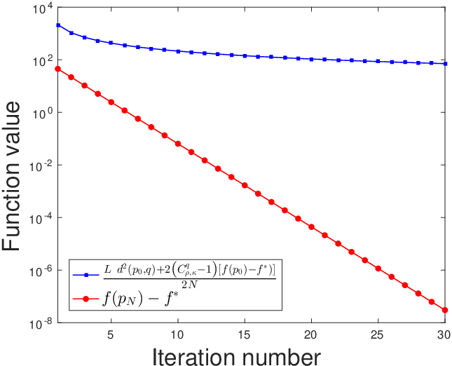
Due to the closed-form solution, we use problem (41) to illustrate the results on iteration-complexity bound of Section 3.2. We consider the Riemannian gradient algorithm with Lipschitz stepsize. Note that the set of positive definite diagonal matrices can be identified with . Thus, problem (41) can be seen as a particular case of problem (37) for positive definite diagonal matrices. Given and defining for all , we defined the Lipschitz stepsize as in Section 5.2.2.
We set , and randomly generated the elements of and initial point from a uniform distribution on . The computed Lipschitz stepsize was set to . The Riemannian gradient algorithm stopped declaring “solution was found” with 30 iterations. Figures 4 (a) and (b) report the function values of the left and right hand sides of inequalities (16) and (17), respectively.
(a)

(b)
6 Conclusions
In this paper, the behavior of the gradient method for convex optimization problems on Riemannian manifolds with lower bounded sectional curvature were analyzed. We considered three different finite procedures for determining the stepsize, namely, constant stepsize, adaptive procedure and Armijo’s procedure. As far as we know, the full convergence of the sequence generated by this method with these three strategies is a new contribution of this paper, which adds important results in the available convergence theory. Besides, under mild assumptions, we showed that the iteration-complexity bound related to the method is for finding a point such that . The numerical experiments provided illustrate the effectiveness of the method in this new setting and certify the conclusions suggested by the theoretical results. Despite the simple linesearch mechanisms employed here, the numerical results indicate that, as it has to be expected, the efficient implementation of linear search algorithms can significantly improve the Riemannian gradient method. In particular, the effectiveness of the method to find the Riemannian mass center and the so-called Karcher’s mean is presented, indicating that the adaptive procedure is a promising scheme that is worth considering. We expect that this paper will contribute to the development of studies of optimization methods in the Riemannian setting. Finally, it would be interesting to analyze stochastic versions of the the gradient method by using adaptive procedures.
References
- [1] P.-A. Absil, R. Mahony, and R. Sepulchre. Optimization algorithms on matrix manifolds. Princeton University Press, Princeton, NJ, 2008. With a foreword by Paul Van Dooren.
- [2] B. Afsari, R. Tron, and R. Vidal. On the convergence of gradient descent for finding the Riemannian center of mass. SIAM J. Control Optim., 51(3):2230–2260, 2013.
- [3] T. Ando, C.-K. Li, and R. Mathias. Geometric means. Linear Algebra and its Applications, 385:305–334, 2004.
- [4] A. Beck and M. Teboulle. A fast iterative shrinkage-thresholding algorithm for linear inverse problems. SIAM J. Imaging Sci., 2(1):183–202, 2009.
- [5] G. C. Bento, S. D. B. Bitar, J. X. Cruz Neto, P. R. Oliveira, and J. C. Souza. The steepest descent method for computing riemannian center of mass on hadamard manifolds. Technical report, submitted, 2017.
- [6] G. C. Bento, O. P. Ferreira, and J. G. Melo. Iteration-Complexity of Gradient, Subgradient and Proximal Point Methods on Riemannian Manifolds. J. Optim. Theory Appl., 173(2):548–562, 2017.
- [7] D. A. Bini and B. Iannazzo. Computing the Karcher mean of symmetric positive definite matrices. Linear Algebra Appl., 438(4):1700–1710, 2013.
- [8] N. Boumal, P.-A. Absil, and C. Cartis. Global rates of convergence for nonconvex optimization on manifolds. ArXiv e-prints, 1(1):1–31, 2016.
- [9] R. Burachik, L. M. G. Drummond, A. N. Iusem, and B. F. Svaiter. Full convergence of the steepest descent method with inexact line searches. Optimization, 32(2):137–146, 1995.
- [10] J. da Cruz Neto, L. De Lima, and P. Oliveira. Geodesic algorithms in riemannian geometry. Balkan J. Geom. Appl, 3(2):89–100, 1998.
- [11] J. X. da Cruz Neto, L. L. de Lima, and P. R. Oliveira. Geodesic algorithms in Riemannian geometry. Balkan J. Geom. Appl., 3(2):89–100, 1998.
- [12] J. X. da Cruz Neto, O. P. Ferreira, and L. R. Lucambio Pérez. Contributions to the study of monotone vector fields. Acta Math. Hungar., 94(4):307–320, 2002.
- [13] M. P. do Carmo. Riemannian geometry. Mathematics: Theory & Applications. Birkhäuser Boston, Inc., Boston, MA, 1992. Translated from the second Portuguese edition by Francis Flaherty.
- [14] E. D. Dolan and J. J. Moré. Benchmarking optimization software with performance profiles. Mathematical programming, 91(2):201–213, 2002.
- [15] A. Edelman, T. A. Arias, and S. T. Smith. The geometry of algorithms with orthogonality constraints. SIAM J. Matrix Anal. Appl., 20(2):303–353, 1999.
- [16] O. P. Ferreira, A. N. Iusem, and S. Z. Németh. Concepts and techniques of optimization on the sphere. TOP, 22(3):1148–1170, 2014.
- [17] D. Gabay. Minimizing a differentiable function over a differential manifold. J. Optim. Theory Appl., 37(2):177–219, 1982.
- [18] B. Jeuris, R. Vandebril, and B. Vandereycken. A survey and comparison of contemporary algorithms for computing the matrix geometric mean. Electron. Trans. Numer. Anal., 39:379–402, 2012.
- [19] S. Lang. Fundamentals of differential geometry, volume 191 of Graduate Texts in Mathematics. Springer-Verlag, New York, 1999.
- [20] C. Lenglet, M. Rousson, R. Deriche, and O. Faugeras. Statistics on the manifold of multivariate normal distributions: theory and application to diffusion tensor MRI processing. J. Math. Imaging Vision, 25(3):423–444, 2006.
- [21] C. Li, B. S. Mordukhovich, J. Wang, and J.-C. Yao. Weak sharp minima on Riemannian manifolds. SIAM J. Optim., 21(4):1523–1560, 2011.
- [22] C. Li and J.-C. Yao. Variational inequalities for set-valued vector fields on Riemannian manifolds: convexity of the solution set and the proximal point algorithm. SIAM J. Control Optim., 50(4):2486–2514, 2012.
- [23] D. G. Luenberger. The gradient projection method along geodesics. Management Sci., 18:620–631, 1972.
- [24] J. H. Manton. A framework for generalising the Newton method and other iterative methods from Euclidean space to manifolds. Numer. Math., 129(1):91–125, 2015.
- [25] Y. Nesterov. Introductory lectures on convex optimization, volume 87 of Applied Optimization. Kluwer Academic Publishers, Boston, MA, 2004. A basic course.
- [26] Y. Nesterov. Gradient methods for minimizing composite functions. Math. Program., 140(1, Ser. B):125–161, 2013.
- [27] Y. E. Nesterov and M. J. Todd. On the Riemannian geometry defined by self-concordant barriers and interior-point methods. Found. Comput. Math., 2(4):333–361, 2002.
- [28] T. Rapcsák. Smooth nonlinear optimization in , volume 19 of Nonconvex Optimization and its Applications. Kluwer Academic Publishers, Dordrecht, 1997.
- [29] M. Raydan. The Barzilai and Borwein gradient method for the large scale unconstrained minimization problem. SIAM J. Optim., 7(1):26–33, 1997.
- [30] O. S. Rothaus. Domains of positivity. Abh. Math. Sem. Univ. Hamburg, 24:189–235, 1960.
- [31] T. Sakai. Riemannian geometry, volume 149 of Translations of Mathematical Monographs. American Mathematical Society, Providence, RI, 1996. Translated from the 1992 Japanese original by the author.
- [32] S. T. Smith. Optimization techniques on Riemannian manifolds. In Hamiltonian and gradient flows, algorithms and control, volume 3 of Fields Inst. Commun., pages 113–136. Amer. Math. Soc., Providence, RI, 1994.
- [33] S. Sra and R. Hosseini. Conic geometric optimization on the manifold of positive definite matrices. SIAM J. Optim., 25(1):713–739, 2015.
- [34] C. Udrişte. Convex functions and optimization methods on Riemannian manifolds, volume 297 of Mathematics and its Applications. Kluwer Academic Publishers Group, Dordrecht, 1994.
- [35] X. Wang, C. Li, J. Wang, and J.-C. Yao. Linear convergence of subgradient algorithm for convex feasibility on Riemannian manifolds. SIAM J. Optim., 25(4):2334–2358, 2015.
- [36] X. M. Wang, C. Li, and J. C. Yao. Subgradient projection algorithms for convex feasibility on Riemannian manifolds with lower bounded curvatures. J. Optim. Theory Appl., 164(1):202–217, 2015.
- [37] Y.-x. Yuan. Step-sizes for the gradient method. In Third International Congress of Chinese Mathematicians. Part 1, 2, volume 2 of AMS/IP Stud. Adv. Math., 42, pt. 1, pages 785–796. Amer. Math. Soc., Providence, RI, 2008.
- [38] H. Zhang, S. J. Reddi, and S. Sra. Fast stochastic optimization on Riemannian manifolds. ArXiv e-prints, pages 1–17, 2016.
- [39] H. Zhang and S. Sra. First-order methods for geodesically convex optimization. JMLR: Workshop and Conference Proceedings, 49(1):1–21, 2016.