Why initial system-environment correlations do not imply the failure of complete positivity: a causal perspective
Abstract
The common wisdom in the field of quantum information theory is that when a system is initially correlated with its environment, the map describing its evolution may fail to be completely positive. If true, this would have practical and foundational significance. We here demonstrate, however, that the common wisdom is mistaken. We trace the error to the standard proposal for how the evolution map ought to be defined. We summarize this standard proposal and then show that it sometimes fails to define a linear map or any map at all. Further, we show that these pathologies persist even in completely classical examples. Drawing inspiration from the framework of classical causal models, we argue that the correct definition of the evolution map is obtained by considering a counterfactual scenario wherein the system is reprepared independently of any systems in its causal past while the rest of the circuit remains the same, yielding a map that is always completely positive. In a post-mortem on the standard proposal, we highlight two distinct mistakes that retrospectively become evident (in its application to completely classical examples): (i) the types of constraints to which it appealed are constraints on what one can infer about the final state of a system based on its initial state, where such inferences are based not just on the cause-effect relation between them—which defines the correct evolution map—but also on the common cause of the two; (ii) in a (retrospectively unnecessary) attempt to introduce variability in the input state, it inadvertently introduced variability in the inference map itself, then tried to fit the input-output pairs associated to these different maps with a single map.
1 Introduction
Quantum state evolution is typically represented by a completely positive linear map. There are two justifications that are usually given for this. The first (the axiomatic justification) is that one always has the freedom to implement a quantum evolution map on a subsystem of some composite system, and complete positivity is then required in order for the state of the composite to remain positive, which is in turn required in order for the Born rule to return positive numbers as the probabilities for the outcomes of future measurements on the system. The second justification notes that the evolution of an isolated system is always described by a unitary map. This implies that the most general sort of evolution of an open system arises by unitarily coupling the system to an environment (in some fixed state) and then tracing over the environment, and such evolution is always represented by a completely positive map.
However, the common wisdom in the field of quantum information is that there is an exception to the rule that the evolution of quantum states is represented by completely positive maps, namely, when the initial state of the system-environment composite does not factorize. For instance, Nielsen and Chuang [[1], Sec. 8.5] state that
“a quantum system which interacts with the degrees of freedom used to prepare that system after the preparation is complete will in general suffer a dynamics which is not adequately described within the quantum operations formalism”,
(here, “quantum operations” refer to completely positive trace-preserving linear maps), and that
“It is an interesting problem for further research to study quantum information processing beyond the quantum operations formalism.”
A large body of literature has arisen to address this problem [2, 3, 4, 5, 6, 7, 8, 9, 10, 11, 12, 13, 14, 15, 16, 17, 18, 19, 20]. This literature includes a great diversity of examples to support the claim that quantum state evolution cannot always be described by a completely positive map from initial to final states of the system.
Some recent work in the literature, e.g. Ref. [21, 22], has criticized non-completely positive maps on the grounds that they lack operational significance. These authors then advocate for a more operational approach (building on Refs. [23, 24]), introducing an alternative framework that avoids the issue of non-complete positivity by proposing a different type of map [25, 26, 21, 22, 27, 28] as representing the evolution of the system. The relation between this prior work and our own proposal is discussed in Sec. 7.2.
Here, we take a more radical stance against non-completely positive maps, arguing that they are explicitly at odds with the standard notion of evolution from elsewhere in physics, a fact that we highlight by taking the perspective of causal modeling. In particular, we do not assume that the evolution of a quantum state is constrained by the marginal states of the system before and after the evolution, as has previously been assumed; indeed, we show that this constraint does not hold.
In the framework of classical causal models, the evolution of a system in any setting is described by ‘do-conditionals’ [29]. These were introduced to describe the inferences that can be made from one variable to another based solely on their cause-effect relation, even when these variables also exhibit correlations due to a common cause. In particular, the correlations that arise between the initial and final versions of a system undergoing Markovian evolution is an example of correlations based solely on a cause-effect relation, whereas correlations between the initial and final versions of a system when the system is initially correlated with an environment with which it subsequently interacts are an example of correlations that are due to both a cause-effect and a common-cause relation. The presence of a nontrivial common cause relation changes the sorts of inferences one can make about the final version of the system based on knowledge of the initial version of the system, but the map describing such inferences does not describe the system’s evolution.
Our criticism of the standard proposal for how to define an evolution map rests on the fact that for purely classical examples, it contradicts the answer that one obtains by defining an evolution map in the presence of initial system-environment correlations using a do-conditional, as the framework of causal inference would have us do. The thrust of our paper is to argue that once one separates out inference and influence, one sees that the mathematical relation that the standard proposal focuses on has no relevance for the map which describes the dynamics of the system; it need not constrain the evolution map in any way. This is in explicit contradiction with the common wisdom.
Consequently, we argue that the common wisdom is mistaken, and that the evolution of a quantum system in time is always represented by a linear and completely positive map. Our definition of the evolution map, therefore, does not lead to any of the pathological conclusions of the standard proposal, such as the failure of complete positivity, the failure of linearity or the failure to define a map.
Pearl has expressed a dictum regarding what counts as a satisfactory resolution of an apparent paradox [30], namely, that the resolution should allow one to retrospectively identify why there was an appearance of paradox. The framework of causal modelling allows us to identify two distinct mistaken assumptions in the standard proposal and to understand precisely how the pathological conclusions arise from these mistakes.
We show that the correct evolution map depends on the marginal state of the environment, but does not depend on the correlations between the system and the environment. This fact is derived from our conception of evolution, and is not assumed a priori. Further, it holds true regardless of the nature of the correlations or the operational procedure by which the initial state was prepared.
Pursuing a quantum generalization of the classical framework of causal modelling has already had many interesting applications in quantum foundations, including: revealing a quantum advantage for causal inference [31], uncovering new experimental scenarios wherein there is a gap between quantum and classical correlations [32, 33, 34, 35, 36, 37, 38], uncovering a promising approach to achieving a causal explanation of Bell inequality violations without fine-tuning [39, 40, 41, 42, 43], expanding the set of experimental configurations wherein one can achieve quantum state pooling [44], and exploring the possibility of quantum uncertainty about the causal structure [45, 46, 47].
This article continues this trend by showing that the correct definition of a quantum evolution map in the presence of initial system-environment correlations requires a quantum generalization of a key notion from classical causal modelling, that of the do-conditional, thereby demonstrating the conceptual significance of the quantum version of this notion.
1.1 Outline of the paper
Section 2 lays out the standard argument for the inadequacy of completely positive maps for describing evolution, abstracted from the various perspectives on the subject found in the literature. The argument is based on a proposal, which we term the standard proposal, for how to define the evolution map in the scenarios of interest. We give several examples in which the standard proposal leads to problematic conclusions, and we explain why these conclusions cast doubt on the validity of the proposal.
In Section 3, we show that the pathological consequences of the standard proposal arise even in purely classical scenarios. In Section 4, we describe how to define a classical evolution map in the presence of initial system-environment correlations, using the notion of do-conditionals from the framework of classical causal models. In Section 5, we show that the prescription of the standard proposal generally fails to reproduce it, and we leverage the framework of classical causal models to elucidate the underlying mistaken assumptions within the scope of classical scenarios.
In Section 6, we show that the definition of the classical evolution map in terms of do-conditionals generalizes naturally to a definition of the quantum evolution map, which is seen to be always completely positive and to avoid the pathologies of the standard proposal. We then assess the mistakes of the standard proposal in the quantum sphere.
Finally, in Section 7 we discuss some of the implications of our definition of the quantum evolution map, we explain how it can be extracted from experimental data, and we advocate for the study of open-system dynamics from the causal modelling perspective.
2 Problems with the standard proposal
2.1 Preliminaries
First we recall some mathematical facts. Let denote the space of linear operators on the Hilbert space describing system . We denote a map from to by . Such a map is said to be trace-preserving if . It is said to be positivity-preserving, or simply positive, if it takes all positive operators to positive operators, . It is said to be completely positivity-preserving, or simply completely positive, if its action on a composite system is also positive; that is, for any ancillary system, denoted at the initial time and at the final time, and evolving by the identity map, , we have .
Suppose that the principal system is coupled to an ancillary system by a unitary , that is prepared at the initial time in the state and that one traces over the ancillary system to obtain the final state of the principal system. The evolution of the principal system is then represented by the map defined by
| (1) |
Note that throughout this article we denote the argument of a map by , where the subscript specifies the type of system at the input. Clearly, such a map is completely positive and trace-preserving. It turns out, furthermore, that any completely positive trace-preserving map can be realized in this fashion, a result known as the Stinespring dilation theorem [48].
2.2 The standard argument for the inadequacy of completely positive maps
We now review the standard argument for the inadequacy of completely positive maps in describing the evolution of the quantum state of the principal system (which we henceforth simply call ‘the system’) when it is initially correlated with the environment [1, 2, 3, 9, 8, 12, 11, 15, 5, 23, 13, 17, 6, 7].
To assume that the system and environment are initially correlated is to assume that their joint state does not factorize, that is, . The system and environment are imagined to subsequently interact according to the map
| (2) |
where is a unitary operator. This scenario is depicted in Fig. 1.

The standard argument is predicated on a particular proposal for how to define the evolution map from to , which we call the standard proposal. (We will argue in the following that the standard argument is mistaken precisely because the standard proposal is conceptually misguided.) The standard proposal begins by assuming that the evolution map, which we denote here by , is constrained by the following equation:
| (3) |
where denotes the marginal on ,
| (4) |
and denotes the marginal on ,
| (5) |
However, Eq. (3) only specifies how a single state of the system, namely , is transformed. This is clearly not sufficient to determine how an arbitrary state on is transformed, and therefore Eq. (3) does not serve to define a map uniquely.11 1 In particular, any pair of states and is consistent with the map that ignores the state of and simply prepares , .
In order to define a map uniquely, it is critical that its action be specified on many different input states. Towards this end, most articles on the topic do not consider a single joint state on system and environment, but rather a set of such states with differing marginal states for the system. The specific means by which this variation is generated differs among proposals: one might apply a transformation on the system, or one might apply a joint transformation on the system and the environment, or one might imagine performing some non-destructive measurement on the system. Physically, it must be that some sort of laboratory operation induces variation on the initial system-environment state. We denote the random variable which encodes the setting of this operation by and the random variable which encodes its outcome by . For each pair of values for these variables, the system-environment composite is prepared in a corresponding state .
The general circuit diagram representing the class of scenarios studied in the literature, then, is that of Fig. 2.

The standard proposal asks us to consider the mathematical relation
| (6) |
where
| (7) |
and
| (8) |
which we term the input-output relation. It asserts that the evolution map should satisfy the constraints
| (9) |
Note that one could only hope to uniquely define a map on all input states in this manner if the map is assumed to be linear and the domain of the input-output relation includes an informationally complete set of states (i.e., the set forms a basis of the operator space ).
The standard argument for the inadequacy of completely positive maps for describing the evolution of the quantum state of the system is concluded by noting that in many scenarios, the map which is defined by Eq. (9) fails to be completely positive. We provide a simple example of this type in the next section.
In fact, one can find examples wherein the prescription that is endorsed by the standard argument defines a map that is not linear, and other examples where it does not define any map at all. We provide such examples in the two subsequent sections. For each type of failure—the failure of complete positivity, the failure of linearity, and the failure to define a map—we explain why it casts doubt on the standard argument.
Before moving to these examples, we pause to note a problematic feature that lies at the very base of the standard proposal.
The question that we believe ought to be answered is the following one:
: What is the evolution map from to in the experimental scenario of Fig. 1?
However, the standard proposal immediately substitutes this question for a new one:
: What is the evolution map from to in the experimental scenario of Fig. 2?
As noted earlier, the motivation for the substitution is that there seems to be no way to answer question if one is committed to the standard proposal, that is, if one is committed to defining the evolution map using an input-output relation for the input states that are realized in the scenario at hand. We will ultimately argue that this commitment is mistaken and that there is consequently no need to retreat from to . For the moment, however, we wish simply to note a problem with any such retreat. Namely, it implies a violation of a criterion of universality that we believe ought to be upheld in such investigations:
Any proposal for the evolution map should be applicable to any scenario.
In particular, it should be applicable to the natural scenario depicted in Fig. 1.
2.3 An example where the standard proposal implies a map that is not completely positive
Imagine that one achieves a variation over the initial state of the system-environment composite as follows: one first prepares it in the maximally entangled state with the environment, , and then for each value of a setting variable , one implements upon it the binary-outcome measurement associated to the orthogonal basis with von Neumann-Lüders state update rule and one post-selects on obtaining the first outcome, . Here, and form an orthogonal basis for the qubit Hilbert space.
This scenario is depicted in Fig. 3. The part of the circuit that is conceptualized as the preparation of the joint state of system and environment (that is, the part which corresponds to the first gate in Fig. 2) is highlighted by a dashed box. This convention is followed in all of the examples we consider.

Because the environment is initially correlated with the system, the state that one infers for it from the post-selection depends on the basis choice and the outcome, a phenomenon that is often termed quantum steering [50, 51]. Specifically, when one learns from the measurement that the quantum state of the system is , one infers that the state of the environment is , where denotes transposition in the computational basis (since for any ).
Thus by varying the parameter and conditioning on obtaining the first outcome of the measurement, , one obtains the set where
| (10) |
The subsequent system-environment interaction is presumed to implement the swap operation on their states. That is, is defined, via Eq. (2), by the operator
| (11) |
where for all and .
By Eq. (8), we infer that the marginal states of the system (for each value of ) after the system-environment interaction are given by
| (12) |
The input-output relation in this case, therefore, is
| (13) |
If the projectors form a basis for the operator space (i.e., an informationally complete set), one can conclude that there is a unique linear map defined (via Eq. (9)) by this relation, namely, the transpose map. This is the canonical example of a map that is positive but not completely positive [1].
i Problematic implications of the failure of complete positivity
Even though the failure of completely positivity is obviously acknowledged by proponents of the standard argument (it is the reason this field of research even exists), we believe that it already provides good reasons for being suspicious of the argument.
An immediate worry is that such maps could lead to output states on system-ancilla composites that fail to be positive.
The standard response to this worry (found, for instance, in Ref. [9, 8]) is that the map describing the evolution of the system in this circumstance is only applicable on a limited domain of input states, and that this domain of input states does not include the marginals of the set of entangled states which manifest the failure of the map to be completely positive.
Note, first of all, that this response is a denial of the axiomatic justification of complete positivity which we discussed in the introduction. The problem we see with this denial is that it forces one to give up on the notion that the map describing the evolution can support inferences about counterfactuals. This notion is central to the notion of evolution in physics: laws of motion are not just descriptions of historically actual motions, but prescriptions for determining what motion would occur for any initial condition. The possibility of making inferences about counterfactual scenarios is precisely what makes laws of motion so useful in practice. To entertain the idea that a map only describes the evolution of a system when that system is assured to be in one of a restricted set of states is to retreat from the usual conception of an evolution map.
2.4 An example where the standard proposal implies a map that is not linear
The following example is a simplified version of the one presented in Nielsen and Chuang [1].
Here, one begins with the product state and, conditioned on the classical control , one applies a controlled-Hadamard gate on the system and a controlled-NOT gate on the environment. This procedure does not involve any measurement, and hence is trivial. The system-environment composite is therefore prepared in one of the states where
| (14) | ||||
| (15) |
with .
Next, there is a controlled- gate with the environment qubit as control and the system qubit as target,
| (16) |
where denotes the unitary gate obtained by performing the Hadamard gate followed by the Pauli gate .
This circuit is shown in Fig. 4.
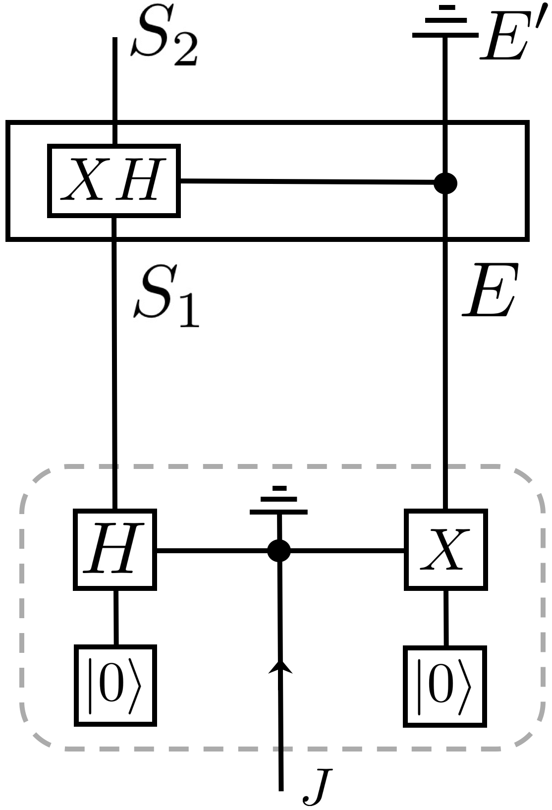
By Eq. (8), we infer that the marginal states of the system after the system-environment interaction (for each value of ) are given by
| (17) | ||||
| (18) |
The input-output relation in this case, therefore, is
| (19) | ||||
| (20) |
Note that the map implied by the standard proposal is not completely specified by these constraints. However, any map consistent with this relation must take nonorthogonal states to orthogonal states, and every such map is nonlinear. (Note that once one allows for the failure of linearity, even having a set of input states that span becomes insufficient to determine how the map acts on all states.)
i Problematic implications of the failure of linearity
The fact that the standard proposal does not always define a linear map is troubling, because the linearity of transformations can be justified on numerous physical grounds. For example, representing a process by a nonlinear map violates the principle that processing of a system cannot increase the amount of information it contains about another system. Specifically, every such map violates the data processing inequality [1]. Such violations have physically problematic implications, such as the possibility of superluminal signalling [52, 53, 54].
2.5 An example where the standard proposal implies a relation that is not a map
Most pathologically, the standard proposal can yield a relation which is inconsistent with any map whatsoever. This is illustrated by a simple example, motivated by one from Ref. [5] and pictured in Fig. 5.

Here, is again trivial, and for each value of , one prepares a distinct initial joint state by performing a controlled-NOT gate on the system with as the control. In this way, the system-environment composite is prepared in one of the states , namely
| (21) | ||||
| (22) |
Next, there is a controlled-NOT gate with the environment qubit as control and the system qubit as target, with unitary description
| (23) |
By Eq. (8), we infer that the marginal states of the system (for each value of ) after the system-environment interaction are given by
| (24) | ||||
| (25) |
The input-output relation defined by this scenario is
| (26) |
Because this relation is one-to-many, it does not define a map from to .
i Problematic implications of the failure of the standard proposal to define a map
The standard proposal purports to define the evolution map. However, we have just seen that it sometimes fails to define any map whatsoever. This failure strikes us as a decisive criticism. Proponents of the standard proposal have not offered any satisfactory account of how their scheme can be salvaged in the face of this failure.
2.6 Every pathology can be obtained from every circuit type
We have provided three examples which illustrate distinct pathologies of the standard proposal. Much previous work [2, 3, 4, 9, 8, 15, 12, 11, 23, 13, 17, 6, 7] has focused on these distinctions, e.g., by seeking necessary or sufficient conditions for the relation to define a completely positive map, a linear map, and so on. The coming analysis shows that these questions are misguided: evolution maps are always completely positive, and all of the apparent counterexamples are really just indicative of the fact that the standard proposal is not the correct way to define the evolution map.
Our examples differed also in the way in which they introduced variability in the initial state of the system-environment composite. Specifically, the variability was introduced (respectively) by (a) the choice of transformation on the system-environment composite, (b) the choice of measurement on the system and the choice of post-selection on its outcomes, and (c) the choice of transformation on the system alone. Roughly, all examples in the literature fit into one of these three special cases of the circuit of Fig. 2. Some articles, however, left the operational (circuit) description of the problem unspecified [15, 8, 9, 12, 5, 11, 13, 6], and took the problem description to be a (possibly continuous) set of initial states on and a unitary system-environment interaction, . One consequence of our work is to show that this version of the problem is not well-posed; knowing the causal structure of the circuit is in fact critical to defining the evolution map.22 2 There is, however, some prior acknowledgement of the importance of the form of the circuit in Refs. [24, 23].
Apart from their simplicity, there is nothing special about the examples we have chosen. In Appendix A, we show that each of the three circuit types can generate each of the pathologies of the standard proposal. In particular, this means that one cannot evade such pathologies by restricting attention to one of the three special classes of circuits.
As we argued at the end of Sec. 2.2, any sensible definition of the evolution map should satisfy a criterion of universality, namely, that it should be applicable regardless of the scenario. As we already noted in that section, the standard proposal fails to satisfy this criterion because it does not define an evolution map in the simple scenario of Fig. 1. We are also not satisfied with the standard responses to the problematic implications of the standard proposal just outlined, because they too compromise on the criterion of universality. Indeed, they do so in a particularly unsatisfying way. Namely, they assert that their proposed definition of the evolution map is only applicable to a restricted class of circuits, but the restriction is ad hoc insofar as no justification is given other than to avoid the pathologies that would otherwise result. For example, Refs. [55, 18] recognized that certain scenarios yielded the pathology discussed in Section 2.5, and sought to avoid it by excluding such scenarios by fiat.
3 Persistence of the problems of the standard proposal in the classical sphere
In a classical setting, one can also consider the evolution map for a system when there are initial correlations between the system and environment. In this section, we demonstrate that if one tries to define this classical evolution map using the prescription endorsed by the standard proposal, then one obtains all of the same problematic implications that one saw quantumly. (This should already be evident given that for many of the quantum examples we presented, both above and in the appendix, all the states and maps could be dephased in the computation basis without affecting our conclusions.) Therefore, although it is a widely held belief that the surprising form of quantum evolution maps in cases of initial system-environment correlations is just another example of a counterintuitive feature of quantum theory (so-called ‘quantum weirdness’), we will demonstrate that it should be taken instead as evidence of the fallacy of the standard proposal for how to define the evolution map.
3.1 Classical Preliminaries
A classical system is described by a set of physical states, which can be encoded as values of a random variable . The statistical state of the classical system is given by a probability distribution over the possible physical states of the system. More precisely, if denotes the set of possible values of (here assumed discrete), then where denotes the probability that . satisfies the normalization condition , where denotes the function on defined by and where the right-hand side of the condition denotes the function that takes value for all .
We are interested in the evolution of these probability distributions for a system interacting with an environment. We will denote the space of probability distributions on by , and for later convenience we introduce the following notation:
| (27) | ||||
| (28) |
A map is called stochastic if there exists a conditional probability distribution such that
| (29) |
Note that this is a linear map.
The most general manner in which a probability distribution on a classical system can evolve is by a stochastic map. This can be justified, analogously to complete positivity in the quantum case, as follows: if one imagines that an ancillary system is prepared in some fixed distribution, and the system-ancilla composite is subjected to a deterministic dynamics, and then the ancilla is ignored, then the resulting map on the probability distribution over the system is always stochastic. Stochastic maps are also the most general type of map that preserve positivity for all input distributions.
3.2 What the standard proposal stipulates in a classical scenario
The standard proposal applies just as well to classical scenarios as to quantum scenarios, since the former are a strict subset of the latter, where all operators are diagonal in some fixed basis. A classical scenario can be described by the same sort of circuit as a quantum scenario: one simply replaces quantum states by probability distributions and unitary operations by deterministic functions. Hence we can consider a direct analogy for each of the quantum circuits considered previously.
The classical analogue for the general circuit from Fig. 1 is shown in Fig. 6(a). If one followed the standard proposal, one would demand that a constraint on the evolution map, which we denote by , is:
| (30) |
with and . One would again be compelled to introduce variability in the input state on in a manner analogous to what was done in the quantum sphere in Fig. 2.
The resulting scenario, a classical analogue for the general circuit from Fig. 2, is shown in Fig. 6(b), where represents a stochastic map induced by a deterministic dynamics, so that
| (31) |
for some functions and .

.
Applying the standard proposal to these classical scenarios, one simply computes
| (32) |
and
| (33) |
generating an input-output relation
| (34) |
as in the quantum case. The standard proposal dictates that the map describing the evolution should be taken to be one which satisfies the constraints encoded in this relation; that is, a map for which
| (35) |
As we now show, this prescription for how to define the evolution map leads to the same sorts of pathologies we saw in the quantum case. There exist simple physical scenarios that generate relations which imply maps that are not stochastic, others which imply maps that are not linear, and still others which do not define any map at all.
Our examples of each of the three failures are chosen to be analogous to the corresponding quantum examples. Note that , and are now taken to denote classical random variables rather than being mere labels of systems.
3.3 A classical example where the standard proposal implies a map that is not stochastic
Our example of the failure of stochasticity in a classical system is analogous to our example of the failure of complete positivity in a quantum system (described in Section 2.3) and is realized with a circuit of exactly the same form (shown in Fig. 3).
Consider a system and an environment that each have four possible physical states, so that . The pair are first prepared in the joint distribution . System is then subjected to one of three measurements, determined by the value of a ternary variable , and each measurement having a binary outcome . The measurement determines whether or not, whether or not, and whether or not. labels the outcome wherein is found to be in the given set, and the complementary set. We further imagine that these measurements are not passive, but disturb the value of the system variable. Specifically, the update rule is such that the final state on depends only on and : is prepared in a uniform distribution over the values of in the complementary set to the one that was found in. For instance, if the measurement is done and the outcome occurs, verifying that , then is reprepared in the distribution .
Finally, undergoes a swap operation with .
In our example, we consider only the cases where the outcome is found to be . For each possible value of , the joint distribution on and , , is as follows:
| (36) | ||||
| (37) | ||||
| (38) |
It follows that after the swap operation on the system and environment, the marginal state of , for each value of and for , denoted , is as follows:
| (39) | ||||
| (40) | ||||
| (41) |
The input-output relation, therefore, is
| (42) |
This relation is consistent with a linear map,
| (43) |
where the probability distribution over the four physical states of is expressed as a vector, . However, this map is not stochastic (e.g., the columns do not each sum to one), and in fact there is no stochastic map consistent with the relation above. To see this, note that the first ordered pair in guarantees that physical state 0 has no probability of mapping to 0 or 1, the second ordered pair guarantees that it has no probability of mapping to 0 or 2, and the third ordered pair guarantees that it has no probability of mapping to 0 or 3. But every stochastic map is certain to map physical state 0 to some other physical state, in contradiction with these three constraints.
3.4 A classical example where the standard proposal implies a map that is not linear
Next, we provide a classical example in which the standard proposal yields a map that fails to be linear. This is analogous to the failure of linearity in the quantum example of Section 2.4, and it is realized in a classical circuit of exactly the same form (shown in Fig. 4).
The system-environment composite is prepared in one of two possible states, depending on the value of :
| (44) | ||||
| (45) |
The system-environment composite then undergoes the following joint evolution: if , then , while if , then , where denotes summation modulo . (Note that the principal system has three distinct states in this example.)
The marginal states of the system (for each value of ) after the system-environment interaction are given by
| (46) | ||||
| (47) |
The input-output relation defined by this transformation is
| (48) |
Any map consistent with this relation must take overlapping distributions to non-overlapping distributions, and every such map is nonlinear.
3.5 A classical example where the standard proposal does not define a map
Finally, we provide a classical example in which the standard proposal fails to yield any map at all. This is an exact analogue of the quantum example of Section 2.5, so it is realized in a classical circuit of exactly the same form (shown in Fig. 5).
As in the quantum example, is trivial, and for each value of , one prepares a distinct initial joint state by performing a controlled-NOT gate on the system. In this way, the system-environment composite is prepared in one of the distributions , namely,
| (49) | ||||
| (50) |
As before, the system-environment interaction is a controlled-NOT gate with the environment qubit as control and the system qubit as target, so that if , then , while if , then .
The marginal states of the system (for each value of ) after the system-environment interaction are given by
| (51) | ||||
| (52) |
The corresponding input-output relation is
| (53) |
Since it is one-to-many, there is no map consistent with this relation.
3.6 Every classical pathology can be obtained from every classical circuit type
We have designed these specific classical examples to make the point as simply as possible (while maintaining a close analogy with the three quantum examples presented previously). As we show in Appendix B, however, there are infinite families of examples which exhibit each of the three pathologies, no matter which type of operational scenario (, and in Section 2.6 above) one considers. These generic classical examples are analogous to the generic quantum examples in Appendix A.
4 The correct definition of the evolution map in the classical sphere
In the quantum literature, some of the problematic examples we described earlier led researchers to question the notion that the evolution of quantum states is always described by a completely positive map. By contrast, no one has previously seen fit to cite the kinds of problematic classical examples that we have just described as a reason to question the claim that evolution of classical probability distributions is always described by a stochastic map. Why not? Could it simply be a failure to recognize the existence of problematic classical examples?
No. The reason no one has questioned the adequacy of stochastic maps is because in the classical sphere no one was inclined to endorse the classical analogue of the standard proposal for how to define the evolution map. Rather, the framework of causal modeling and the so-called do calculus was developed [29], and this provided a scheme for inferring the evolution map on the system even in the presence of initial correlations between system and environment. It is found to differ significantly from that of the standard proposal, and in particular it avoids all of the problematic implications. In this section, we will present this scheme, explain why it clearly yields the correct notion of an evolution map in the classical realm, and identify the mistaken assumptions in the standard proposal.
The correct definition of an evolution map in the classical sphere generalizes easily to the quantum sphere, as we will show in Section 6.
4.1 The causal perspective on defining an evolution map
We begin with some reflections on the notion of an evolution map in a classical statistical theory. These are the ideas that underlie the calculus for causal reasoning that has been developed by Pearl [29]33 3 Classical causal models are typically defined in terms of directed acyclic graphs, rather than circuit diagrams. We use the latter representation because it facilitates the comparison with the quantum case. .
An evolution map is not a mere description of the actual statistical states of the input and the output of a process, but a prescription for determining the statistical state of the output for any statistical state of the input, in analogy to what distinguishes a law of motion from a historical account (as we already noted in Section i). Just as a law of motion is autonomous from the initial conditions, an evolution map is autonomous from the state at its input: for any variation of the state of its input, the map is unchanged.
To define the evolution map from to in an arbitrary circuit, therefore, one considers a counterfactual scenario involving the minimal modification to the circuit which allows one to freely vary the statistical state of , while keeping the rest of the circuit unchanged. This minimal modification consists of altering the causal mechanism that determines , while keeping every other causal mechanism in the circuit unchanged. (We have here made explicit use of the fact that the different causal mechanisms in the circuit are autonomous.) Because the way that depends on is only a function of these other causal mechanisms (and not a function of the mechanism that determines ), it is the same in the counterfactual circuit as it is in the actual circuit. Therefore, the evolution map from to in the actual circuit can be identified with the map from to in the counterfactual circuit. We denote the evolution map from to by , in deference to the notion of a ‘do-conditional’ from classical causal modeling.
Recall the very first scenario we introduced, shown in Fig. 1, and consider its classical analogue, shown in Fig. 7(a). For such a circuit, one computes the evolution map from to by applying the prescription just given, as follows. One imagines that the naturally occurring state of is ignored, and instead a new state for is prepared, in a manner uncorrelated with the systems that would under natural circumstances be its causal parents. The counterfactual scenario being imagined is depicted in Fig. 7(b). The wire labeled in the original circuit is replaced, in the counterfactual circuit, by a pair of wires that are disconnected. The first, which inherits the label , maintains the causal ancestry of the original, but is marginalized over (denoted by the ground symbol from electronics). The second, which is labeled by , maintains the causal descendants of the original, and is an input to the counterfactual circuit.

The evolution map from to in the original circuit of Fig. 7(a), , is defined as the map which is isomorphic (under the identification of and ) to the map in the counterfactual circuit of Fig. 7(b), that is,
| (54) |
The classical causal models framework typically focuses on the do-conditional , rather than the evolution map , but the latter is simply related to the former via
| (57) |
Eq. (56) implies that the evolution map can be computed directly from the identity of the circuit elements in the original circuit of Fig. (1). This is because it depends only on and (which is obtained from by marginalization).
It follows, in particular, that there is no need to consider an input-ouput relation. This is in contrast to the standard proposal, which (because of its insistence on starting with the input-output relation) cannot define a map uniquely unless the scenario explicitly involves a set of initial states. This is why, as we noted in Sec. 2, the standard proposal cannot define a map for the circuit of Fig. (1) and why it is forced to consider circuits of the form of Fig. (2), where there are variables and/or that allow one to introduce variation in the input state.
Note that we are here discussing how to define the evolution map when one has a complete description of the form of the circuit and the identity of each of its elements. The question of how one obtains such a description is not relevant to the definitional question, and it is important not to confuse the two questions. We will discuss the question of how to infer the quantum evolution map from experimental data in Section 7.4.
4.2 Contrasting the evolution map with the inference map
In the causal modeling framework [29], the primary motivation for introducing do-conditionals was to distinguish them from standard conditionals. We pause here to describe the distinction because it is critical to our analysis of the mistakes of the standard proposal.
Suppose that one considers the map defined by the standard conditional , namely,
| (58) |
The correct way of interpreting the map defined in Eq. (58) is as an inference map. It answers the question: Given a particular state of knowledge of , what is the appropriate state of knowledge to assign to ? In particular, if one updates one’s description of (based on passively observing it, for instance), this map specifies how one should update one’s description of . If and are related causally by both a cause-effect connection and a common cause of the two, then the inference map describes what can teach you about through either causal pathway. By contrast, the evolution map specifies only what can teach you about through the cause-effect pathway.
This distinction is often illustrated by Simpson’s paradox. This is a scenario in which there is a positive correlation between a treatment variable and a recovery variable, even though the causal influence of the treatment is to reduce the probability of recovery (see Sec. 6 of [29]). The positive correlation is the result of there also being a common cause acting on the two variables. For instance, if men are more likely than women to seek the treatment and are also more likely than women to recover regardless of treatment, then gender acts as a common cause. In this circumstance, learning that an individual in the sample population got the treatment warrants assigning a higher likelihood to the proposition that that individual recovered, simply because learning that someone got the treatment is positive evidence for them being male, which in turn is positive evidence for them recovering.
To see this mathematically, let denote the recovery variable and let denote the treatment variable. If one naïvely computes , or equivalently, the map (via Eq. (58)), it is clear that this does not represent the cause-effect relation that exists between and and hence cannot be used to make assessments of the effectiveness of the treatment on recovery. Only the map , computed from (via Eq. (57)), wherein the intervention on rules out the possibility of inference via a common cause, represents state updating based purely on the cause-effect relation.
In short, Simpson’s paradox reminds us that correlation does not imply causation. To draw conclusions about whether a given treatment contributes causally to recovery, one must consider what would occur in a trial wherein the value of the treatment variable is assigned at random (drug or placebo, for instance), independently of any preferences of the individual. The do-conditional describes what would occur in such randomized trials.
Hence, we see that the evolution map is generally distinct from the inference map.
Finally, note that—just as we saw for the evolution map—the inference map in classical scenarios can be computed directly from the original circuit elements, so that one need not consider any sort of input-output relation. To see this, first note that the conditional can be expressed as
| (59) | ||||
| (60) |
The assumption that the circuit elements in Fig. 7(a) are known implies that and are known. in the above equation is just the conditional associated to the stochastic map , while can be computed from by where . The inference map associated to the conditional is then found, via Eq. (58), to be:
| (61) |
5 The mistaken assumptions of the standard proposal in the classical sphere
With the causal point of view in mind and the correct definition of the evolution map in hand, it is very instructive to revisit the standard proposal in the classical sphere and to isolate the mistaken assumptions therein.
5.1 The mistake of confusing the evolution map with the inference map
Consider what the standard proposal entails for the simple circuit of Fig. 7(a). There is only a single distribution and a single distribution , and so the input-output relation consists of a single input-output pair, namely, . The standard proposal is committed to the notion that this input-output pair can be interpreted as a constraint on the evolution map, namely, that the evolution map acting on must yield .
Classical probability theory dictates that the relationship which holds between and is
| (62) |
and consequently, if is the stochastic map associated to the conditional by Eq. (58), then
| (63) |
But is the inference map from to , which can differ from the evolution map , as discussed in Sec. 4.2. Consequently, the input-output pair is only guaranteed to be consistent with the inference map and is not guaranteed to be consistent with the evolution map. Indeed, if there is a common cause acting on and , as is the case in the circuit of Fig. 7(a), then generically the evolution map and the inference map do differ, and the input-output pair is only consistent with the inference map and not the evolution map.
To assume, as the standard proposal does, that the input-output pair constitutes a constraint on the evolution map is to make a mistake akin to inferring causation from correlation alone. For instance, it is akin to inferring, from a positive correlation between treatment and recovery, that treatment has a positive causal influence on recovery even though there is a common cause (such as gender) that could account for this positive correlation.
This is the first mistake of the standard proposal.
As we discuss in Appendix C, the inference map and the evolution map coincide if and only if and are marginally independent, . This is ironic, because proponents of the standard proposal were interested in characterizing precisely those scenarios which violated this condition.
5.2 The mistake of taking input-output pairs from different inference maps as constraints on a single map
Proponents of the standard proposal sought to define a map through an input-output relation where variability in the input state of the system (and therefore also the output state of ) was introduced via variation in the values of and in a circuit of the form of Fig. 6(b). Since, as noted in the previous section, an individual input-output pair in is not a constraint on the evolution map, the set of such pairs obviously does not constrain the evolution map either. This would seem to leave open the possibility that the set of input-output pairs might still constrain the inference map. However, this is not the case either. If confusing inference with evolution had been the only mistake of the standard proposal, then because every inference map is a stochastic map, one would never have found any failure of the input-output relation to define a stochastic map, contrary to what is found in the pathological examples.
The standard proposal not only fails to yield the evolution map, it also fails to yield the inference map, due to a second mistaken assumption, which we now discuss.
As we argued in Section 4.2, the inference map in classical scenarios can be computed directly from the circuit, without introducing a set of initial states indexed by and . Therefore, introducing explicit variation in the initial state was unnecessary. Moreover, it is the root of all the pathological implications of the standard proposal.
The means by which variability was introduced in the input state inadvertently led to variability in the inference map as well. That is, for generic examples of circuits to which the standard proposal has been applied (those of the form of Fig. 6(b)), the variation in the values of and leads not only to variation in the marginal state of the system , but also to variation in , and hence, given Eq. (61), to variation in the inference map.
To show this, we determine the formula that relates the conditional probability to for circuits of the form of Fig. 6(b).
By definition,
| (64) |
To express as a function of , we simply make a repeated application of an identity from Bayesian probability theory, namely, . We infer that and consequently that
| (65) |
For a circuit of the form of Fig. 6(b), the causal structure ensures that is conditionally independent of given , so that , and we conclude that
| (66) |
This defines a -dependent map from distributions on to distributions on . Specifically, if we define by
| (67) |
the map is
| (68) |
Rewriting in terms of the circuit elements given in our scenario (as was done in Eq. (61)), this map has the form:
| (69) |
For one who knows that and , the latter map is the correct way of making inferences from to . The inference map clearly depends on the values of and .
It follows from Eqs. (66) and (68) that if and are defined by
| (70) | ||||
| (71) |
then the input-output pair is consistent with the map in the sense that
| (72) |
However, the prescription of the standard proposal was to find a single map such that
| (73) |
This last step is the origin of the pathologies of the standard proposal. As Eq. (72) shows, in general the input-output pairs for different values of describe the input and output states of different maps. But the prescription of the standard proposal asks us to collect all of these input-output pairs into a single set, the input-output relation, and to try and find a single map that is consistent with all of them. Given the origin of these pairs, there is no guarantee that there is any such map, and even if there does happen to be one, there is no guarantee that it is linear or stochastic.
To summarize, the second mistake of the standard proposal is to have inadvertently introduced variability in the inference map and then to have tried to define a unique map from the input-ouput pairs that are associated to these different inference maps.
5.3 The correct evolution map(s) for the scenarios wherein the standard proposal led to pathologies
In the previous section, we noted that the inference map can be -dependent in the scenario of Fig. 6(b). It turns out that the evolution map can also be -dependent in this scenario. Generally, therefore, there is no single evolution map to be characterized in this scenario. Rather, following the prescription of Section 4.1, one finds that for each valuation of and , there is a (generally) distinct marginal state of the environment, which leads to distinct evolution maps, namely
| (74) |
At first glance, this may seem problematic, but in fact the knowledge-dependence of evolution maps is ubiquitous in both classical and quantum physics. We give several examples in Appendix D.
5.4 Illustrating the mistakes with the classical examples considered previously
In this section, we illustrate the general discussion just given by explicitly analyzing classical examples introduced previously, highlighting interesting features along the way.
Consider again the third classical example, discussed in Section 3.5, where the input-output relation failed to identify any map at all.
Recall that the example has no variable, so only is relevant. Consider the inference map from to for a particular value of . Specializing Eq. (69), this has the form
| (75) |
The coupling of system and environment implies that ; that is, it implies that tracks the parity of and . The controlled-NOT operation from to toggles this parity in a -dependent way, but without changing the marginal state of . Thus, as one varies , one has variability in the state on , but no variability in the state on , leading to the one-to-many relation that fails to correspond to any map.
One way to understand the fact that different values of lead to different states on is that is correlated with given , so that , or equivalently (given Eq. (70)), , and consequently the inference map in Eq. (75) becomes -dependent.
Indeed, as we show in Appendix E, the inference maps for the two values of are
| (76) |
so that for (), one updates one’s description of to the state () regardless of one’s state of knowledge of .
Recall the input-output relation for this example, Eq. (53). Clearly, the first () input-output pair is consistent with the inference map for , , while the second () input-output pair is consistent with the inference map for , . However, if one mistakenly considers both input-output pairs to be associated to a single map, one finds a contradiction. This illustrates the second mistake of the standard proposal.
The first mistake of the standard proposal is also illustrated in this example.
The correct evolution map is straightforward to identify using the prescription of Section 4.1. For both values of , the marginal state of the environment is uniformly random, so the evolution map is -independent and equal to the randomizing map
| (77) |
which takes any input probability distribution on to a uniformly random distribution on . This is distinct from either of the inference maps or , and so confirms that the evolution map is not constrained at all by the input-output pairs considered in the standard proposal.
We now turn our attention to the second classical example, discussed in Section 3.5.
Again, only the variable is nontrivial in this example. However, whereas was a cause of alone in the third classical example, here it is a cause of as well. In fact, is the complete common cause of and and consequently is conditionally independent of given , . Thus, Eq. (69) specializes to the expression
| (78) |
for the inference map from to in this example. Different values of lead to different marginals on , and therefore different inference maps.
The inference map for is
| (79) |
as shown in Appendix E. For any state of knowledge of , one should assign the same state of knowledge to if , and the same state of knowledge modulo an increase of the value by 1 (in arithmetic modulo 3) if .
Again, one can check explicitly that in this example an individual input-output pair for , (as in Eqs. (44) and (46)), is a constraint on the inference map for . However, if one mistakenly considers both input-output pairs to be associated to a single map, then the only maps consistent with the constraint are nonlinear.
In this example, it happens that the evolution map for a particular value of coincides with the inference map for that same value,
| (80) |
The reason is that conditioning on makes and independent, so that in the presence of this conditioning, one need not intervene on the system to achieve this independence.
The analysis of the first classical example is similar, and is also provided in Appendix E.
The situation in the classical sphere can be summarized as follows. The only sensible notion of an evolution map classically is the one defined by a do-conditional, but the information used in the standard proposal to try to infer the system’s evolution—input-output pairs of statistical states—does not constrain the evolution map but instead only constrains the inference map. Furthermore, even if one were content to try to identify the inference map rather than the evolution map, the prescription of the standard proposal does not provide a means of doing so because it takes a number of input-output pairs for different inference maps and mistakenly takes them all to be constraints on a single map.
6 The correct definition of the evolution map in the quantum sphere
The definition of a classical evolution map, presented in Section 4, generalizes naturally to the definition of a quantum evolution map. It suffices to substitute the quantum analogues of the relevant classical notions (quantum states for statistical states and unitary dependences for functional dependences) in the definition provided there.
The ideas underlying the definition are the same as those outlined in Section 4.1: an evolution map for quantum states of a system is a prescription for determining the quantum state of the output for any quantum state of the input, and it is autonomous from the state at its input.
Just as in the classical case, one imagines the counterfactual scenario with the minimal modification to the circuit which allows one to freely vary the quantum state of , while keeping the rest of the circuit unchanged; the evolution map from to in the actual circuit can then be identified with the map from to in the modified circuit. We denote an evolution map from quantum system to quantum system by , where the “do” on the right of the conditional parallels the classical notation and is a reminder that the definition requires contemplating the counterfactual scenario just described.
Let us return to the most basic quantum circuit wherein the system and environment are initially correlated, that of Fig. 1, reproduced here as Fig. 8(a). For this case, the relevant counterfactual scenario is depicted in Fig. 8(b). We again denote the version of the system which is varied counterfactually by , and here the ground symbol from electronics represents the trace over a subsystem.

The evolution map from to in the circuit of Fig. 8(a), denoted , is defined as the map which is isomorphic (under the identification of and ) to the map in the counterfactual circuit of Fig. 8(b); that is,
| (81) |
This prescription unambiguously leads one to identify the evolution map to be
| (82) |
where . This is the quantum analogue of Eq. (56). It is always completely positive.
The quantum evolution map can be deduced from the identity of the circuit elements in the original circuit of Fig. 8(a) because it depends only on and on (which is obtained from by taking a partial trace). No input-output relation is needed.
Furthermore, like its classical counterpart, the quantum evolution map is knowledge-dependent insofar as it depends on one’s information about the environment, encoded in the quantum state .44 4 Some previous works (e.g. Refs. [5, 11]) sought to define the evolution map as a function of the marginal state of the environment and also as a function of the initial system-environment correlations present in the initial state of the composite. This prescription is distinct from that of the standard proposal, but it does not correspond to our prescription. In particular, it does not reproduce the correct evolution map (of Eq. (82)) because the latter depends only on the marginal state of the environment. As we discuss in Appendix D, this knowledge-dependence of one’s description of evolution is ubiquitous in physics, including textbook quantum mechanics.
For completeness, in Appendix F we determine the correct evolution map for each of the three quantum examples from Section 2. We also show that the most general circuit considered in the standard proposal, Fig. 2, is described by a distinct evolution map for each valuation of and :
| (83) |
6.1 What is an inference map quantumly?
Once one takes a causal point of view, the description of quantum evolution is scarcely more complicated than the description of classical evolution. Devising a complete framework for describing inference in quantum theory, however, is a much more complicated venture, and remains an open problem [40, 56, 44]. (Note that, in keeping with the framework laid out in section 4, both evolution and inference are formalized as maps from states of to states of , and it is this type of object that we are interested in here. We discuss maps with a more general input type in Section 7.2.)
The root of the problem lies in how one acquires the information about that is input into the map. Classically, passive observation of a variable does not change the dependence of that variable on its causal parents. So, there is a way to update one’s knowledge of , and therefore the distribution , without changing any of the causal mechanisms that relate to the other variables of interest. In the quantum realm, however, it is unclear whether there is an appropriate analogue of passive observation given that every attempt to gain information about a system changes its state. Consequently, it would seem to be impossible to update one’s knowledge of , and therefore the state , without changing any of the causal mechanisms that relate to the other systems of interest. (For example, measuring a quantum system generally leads to a different post-measurement state, altering the way in which the system affects its causal children, while preparing the system in a known state nullifies the influence of its causal parents.)
It is worth noting that, even classically, it is only for a limited set of probing schemes on (which includes ‘passive’ measurements, which are non-disturbing and maximally informative) that the question of what one can infer about (given the outcome of the probing scheme) can be answered by an inference map that takes statistical states on as input. Since this is mathematically a limiting case of the full quantum treatment, one can see already that for quantum systems, too, only a limited set of probing schemes on could possibly admit inferences about that can be expressed by a map with quantum states on as input. Moreover, since quantum states generally contain richer information about a system than their classical limit, the set of scenarios that admit such an inference map is likely to be even more restricted. Nonetheless, it is conceivable that there are intrinsically quantum scenarios—those that cannot be reduced to an effectively classical description—wherein such an inference map can be defined.
For generic probing schemes (both classical and quantum), there is no such map which takes a state of as input.
6.2 The mistakes of the standard proposal in the quantum sphere
The set of quantum states and evolution maps includes the set of classical states and evolution maps as special cases (wherein all operators are diagonal in some fixed basis). The fact that the standard proposal fails to identify the correct evolution map in various classical examples, therefore, implies that it is not a valid prescription for identifying the correct evolution map in the quantum sphere. Furthermore, the mistaken assumptions of the standard proposal that we have identified by considering classical examples remain mistaken assumptions in the quantum sphere.
Outside the classical subtheory, the story is more subtle, but analogues of the two mistaken assumptions can be identified. We begin with the quantum analogue of the first mistake. Although we have left open the question of whether one can make sense of the notion of an inference map from to in such examples, it is still clear that, whenever one has initial system-environment correlations, the quantum systems and are causally related not only as cause and effect but by a common cause as well. As such, an individual input-output pair of states in such a scenario will generally not reflect the cause-effect relation alone. But given that the correct definition of the evolution map depends only on the cause-effect relation, there is no reason to think that an individual input-output pair of states is a constraint on the evolution map when there are initial system-environment correlations.
Indeed, as we show in Appendix G, the necessary and sufficient condition for an individual input-output pair to be a constraint on the evolution map is that the joint state on factorizes, . The ironic conclusion (reached also in our discussion of the classical case) is that the only circumstance in which the first mistake of the standard proposal would be innocuous is the case of no initial system-environment correlations.
If there is (as speculated in the previous section) a subset of intrinsically quantum scenarios where an inference map can be defined, and the scenario in question is presumed to be within this subset, then perhaps an input-output pair of states for a given value of could be taken as a constraint on the inference map. But it would still be the case that the inference map would vary with , and consequently it would be inappropriate to consider all of these input-output pairs as constraints on a single map. This is the second mistake of the standard proposal.
7 Discussion and Future Work
We here summarize some of the lessons of our analysis. First, one cannot define an evolution map simply by listing a set of marginal states at its input and at its output, since if there is a common cause acting on the input and the output, then such pairs of states do not constitute constraints on the evolution map. Second, one should not restrict the input domain of the evolution map, as this would violate the counterfactual conception of evolution, embodied for instance in the idea that a law of motion should be autonomous from the initial conditions. Further, such restrictions are not needed to preserve complete positivity. Third, the marginal state of the environment is relevant to the evolution map, while the system-environment correlations are not. This latter fact is not assumed, but rather is derived from our conception of evolution, and holds true in all possible operational scenarios and for all possible initial states. Fourth, because the marginal state one assigns to the environment describes one’s information about the environment, the evolution map one assigns will depend on one’s state of knowledge. If a scenario includes a variable that contains information about the environment, then that scenario is associated to a set of evolution maps rather than a single evolution map, one for each value of the variable.
We hope that these lessons might be valuable outside the scope of this work.
7.1 Composition of evolution maps
The definition of the quantum evolution map, Eq. (82), has the following feature: for a circuit of the form of Fig. 9, the composition of the evolution map from to with the evolution map from to does not generally yield the evolution map from to ; that is, the compositional property fails to hold.
This compositional property only holds if constitutes the complete causal mediary between and . For the circuit in Fig. 9, however, is also such a causal mediary, and so the only sequential decomposition of the evolution map from to that holds is the decomposition into an evolution map from to and an evolution map from to , that is, .

It is only with the correct definition of the evolution map that one can properly pose the question of how it can be decomposed into a temporal sequence of evolution maps. Therefore, we expect that our results will have relevance to questions about the divisibility of quantum channels and the detection of nonMarkovianity [57, 58].
7.2 Comparison with prior work
As mentioned in the introduction, some prior work has also criticized the standard argument for the inadequacy of completely positive maps [21, 22]. These works have argued against the standard proposal on the grounds that it lacks operational meaning, for instance, by pointing out that one cannot vary the marginal state of the system while keeping the system-environment correlations fixed. In contrast, our criticism of the standard proposal is that (i) it fails to satisfy the criterion of universality, e.g., it only seeks to answer question (concerning Fig. 2) rather than question of Section 2.2 (concerning Fig. 1), and even for question it sometimes fails to identify any map as the description of the evolution of the system; and (ii) in the classical limit, it fails to reproduce the evolution map that is implied by the framework of classical causal modeling.
This prior work, e.g. Refs. [25, 26, 21, 22, 27, 28], has also proposed a new framework for analyzing dynamics in the presence of system-environment correlations, where one focuses on an altogether different type of map that does have a clear operational meaning and which is always completely positive. Specifically, whereas maps purporting to describe the dynamics of system typically take states on as input and have states on as output, these new maps take instruments from to as input and have states on as output. In other words, the domain of the map is the space of operators on two rather than one copy of the system’s Hilbert space, that is, on rather than on .

One can motivate this new perspective by considering the circuit in Fig. 10(a), which is clearly a special case of Fig. 2, and reconceptualizing the experiment not as a preparation of a set of initial joint states on , but rather as an interventional probing scheme on the system. This idea is represented in Fig. 10(b), where the intervention on the system is denoted inside the dashed box, and is associated for each value of and of with a map , and where the circuit fragment outside the dashed box is associated with a map . The circuit fragment defines a map from each element of the instrument describing the intervention, , to a state using the link product of Ref. [59], , where the output of the circuit fragment is fed into the input of the instrument, and the output of the instrument is fed into the input of the circuit fragment. This sort of map has been studied in many formalisms [45, 60, 61, 59, 62, 63, 64, 65, 21] and is often termed a quantum comb [59] or a process matrix [62]. When it was introduced for the study of open quantum systems in Ref. [21], this object was termed the -map.
As we understand it, the formalism of -maps differs from our own framework in two key respects.
Firstly, the -map and our evolution map seem to have been proposed as answers to different questions: the -map was introduced to describe aspects of the system’s dynamics in an experiment of the form of Fig. 10(b), where an intervention is actually made on the system, whereas our proposal is intended to describe the evolution of the system in the natural experiment of Fig. 1. In other words, whereas we aim to answer question from Sec. 2.2 (concerning Fig. 1), the -map is proposed as an answer to a question of the form of , but with the experiment given by Fig. 10(b) (rather than Fig. 2).
Secondly, we have defined the evolution map to be a complete description of the inferences one can make from to based purely on the cause-effect relation between the two, while the -map does not capture only those types of inferences, but, rather includes (as noted in, e.g., Ref. [21]) information about the initial correlations between the system and environment, and hence describes one’s inferences based on both the cause-effect and on the common-cause relation between and . One consequence of this distinction is that our notion of the quantum evolution map reduces in the classical limit (where all operators are diagonal in some fixed basis) to the classical evolution map, which we identify with Pearl’s do-conditional, whereas the -map does not reduce to the do-conditional in the classical limit. Indeed, from our perspective, the very fact that the -map takes an instrument from to as input rather than a state on precludes it from being a candidate for the evolution map.
Ref. [66] also asks a question of type ; namely, it asks what map one should use to describe scenarios in which certain special types of interventions are performed on the system. One such set of interventions considered in Ref. [66] and called ‘stochastic preparations’ consist of a trace operation on and a repreparation of in one of an informationally complete set of states. For such a set of interventions, the map that is tomographically reconstructed from data is
| (84) |
Based on the notation used for this object in Ref. [21], we call it the -map. Unlike the -map, it is identical in form to the evolution map we have introduced in Eq. (82). However, just as we noted in our discussion of the M-map, we read this prior work as asserting that the L-map describes the dynamics only for a very limited scope of experiments, namely, those wherein a ‘stochastic preparation’ was actually implemented and not that it does so for the the general case involving no intervention, depicted in Fig. 1.
This prior work appears to be motivated by a type of operationalism wherein an entity is only meaningful insofar as one can specify the experimental procedure that would allow one to measure it. In particular, it defines both the -map and the -map in terms of the tomographic procedure by which one could identify it. By contrast, the causal modelling perspective that we adopt in this work is not wedded to this positivist notion of meaningfulness and therefore aims to answer question directly, without recourse to interventions, but rather through the use of counterfactuals.
Note, however, that if one adopts the positivist attitude merely as a means for discovering the form of the -map, but one then kicks away this empiricist ladder and simply treats the -map as the correct description of dynamics even in the case of Fig. 1 (where there are no interventions on which any operational definitions could be based), then one comes to the same conclusion regarding the correct definition of the evolution map as we have reached here by adopting the causal modelling perspective.
Similarly, one might appeal to such a ladder-kicking procedure to justify considering the -map as pertinent not just to the class of experiments shown in Fig. 10(b), but also to the general case of Fig. 1. Even reconceptualized in this way, however, the -map is not an evolution map in our sense, for the reasons described above. So what does the map describe from the causal modelling perspective? We address this question in the next section.
7.3 The status of the quantum comb from the causal point of view
Viewed as a description of the general case of Fig. 1, Eq. (84) shows how the map can be used to recover the evolution map, which describes inferences which can be made solely on the basis of the cause-effect relation between and . Additionally, can be used to recover an inference map which describes inferences which can be made solely on the basis of the common cause relation between and . In order to be assured that one’s inferences about are based purely on knowledge of , and not on knowledge of , one presumes a state of complete ignorance regarding , represented by the completely mixed state , where is the dimension of . The object that allows one to make inferences based solely on the common cause relation, therefore, is the joint state
| (85) |
In particular, if one implements a measurement on and one obtains an outcome associated to a positive operator , then one should update one’s description of to
| (86) |
where is a normalization constant. This defines a map from effects on to states on which has been termed the steering map and discussed in [31]. It is linear and co-CP (that is, the composition of the map with the tranpose operation is completely positive).
Based on these facts, one might hope that the map simply represents the elusive quantum inference map that we discussed in Section 6.1. However, it does not.
Here, one must again distinguish between two sorts of maps that might describe such inferences—one whose inputs are operators on a single copy of , and one whose inputs are operators on two copies of . It is the possibility of the former that we discussed in Section 6.1, whereas the map , if it is to be interpreted as an inference map, is of the latter variety. Even if it turns out that the only sort of inference map which can sensibly be defined in generic quantum scenarios has as input a state on 55 5 Which is a reasonable conjecture: even in the classical sphere, disturbing interventions are most naturally described by an inference map from states of knowledge on two copies of random variable to ., the natural inference map would still be of the form , rather than . Defining such a map likely requires a theory of quantum Bayesian inversion (e.g. to determine the correct input state on from a specification of an instrument from to ).
7.4 Experimentally determining quantum combs and evolution maps
Our focus herein has been on elucidating the correct definition of the evolution map when the circuit is completely specified. A secondary problem concerns deducing the evolution map from experimental data. (It is secondary insofar as it can only be addressed once one has the correct definition of the evolution map).
It is clear that if one can experimentally characterize the different components of the circuit (the state and the unitary map ), then one can deduce the evolution map from Eq. (82). Although this is sufficient, it is not necessary for characterizing the evolution map. The question arises, therefore, of what is the minimal experimental effort that suffices.
To begin with, consider the idealization wherein one can perfectly implement any desired laboratory operation. The causal map has input space and output space Hence, if one intervenes on the system by performing an informationally complete measurement on and then repreparing one of an informationally complete set of states on , and one also implements (for each state on ) an informationally complete measurement on , then one can tomographically reconstruct the causal map. This was termed causal tomography in Ref. [31].
If one has experimentally determined the causal map, then the evolution map can be computed directly from it via Eq. (84). A less demanding experimental method, however, is to simply ignore (rather than measuring it) and prepare in one of an informationally complete set of states. For each such state, one then implements an informationally complete measurement on . This achieves process tomography on the evolution map. Note that this corresponds to experimentally implementing the intervention that is contemplated in the counterfactual circuit that defines the evolution map. It is analogous to measuring a classical do-conditional by implementing a randomized trial.
What about experimentally determining the causal map or evolution map when the experimenter does not have ideal laboratory operations? For example, what if they are not able to localize their operations to particular systems, or to characterize their laboratory operations accurately? Because such limitations can result in inadvertently preparing initial system-environment correlations, they have previously served as a motivation for this field. Specifically, it has been suggested that if no completely positive map fits the relation of the standard proposal, this should be taken as evidence that one has inadvertently introduced system-environment correlations [67, 23].
Given our demonstration that the prescription of the standard proposal does not yield the evolution map, we advocate against analyzing experimental data in the manner it proposes, even if only as a diagnostic for imperfections in one’s laboratory operations. The solution to the problem of imperfect laboratory operations is to use a form of tomography in which various features of the probing scheme (such as the identities of the laboratory operations and the dimensionality and nature of the systems being probed) are not presupposed, but are rather taken to be hypotheses whose plausibility is assessed on the basis of the data. In identifying the evolution map that provides the best fit to the experimental data, the maps over which one varies must be constrained to be completely positive (by virtue of the definition of an evolution map), and if the quality of the fit is poor (as is indicated, for instance, by a bad -value), then the correct reaction is not to entertain the possibility that completely positive maps are inadequate for describing evolution, as has previously been suggested [67, 23], but to reject one or more of the assumptions about features of the probing scheme. A demonstration of how to implement tomography in this way is provided in Ref. [68].
Finally, we note that in classical scenarios, it is sometimes possible to identify the evolution map from purely passive observations if these are made on the right systems. (The more general problem of identifying the do-conditional for some pair of variables embedded in a given causal structure is known as the “identifiability problem” [29].) The significance of this fact is that although evolution maps are defined in terms of hypothetical nonpassive interventions, these nonpassive interventions need not necessarily be performed in order to identify the map. Whether there is a sensible quantum analogue of the identifiability problem and whether it is possible to sometimes deduce the quantum evolution map without nonpassive interventions remains unclear. In particular, to even pose the question, one must explore whether there is anything in quantum theory that ought to be considered an analogue of passive observation.
8 Conclusion
We have argued that, for a general circuit wherein a system interacts with its environment such as the one in Fig. 1, the evolution map on the system should be defined as in Eq. (82). This map is always linear and completely positive, even in the presence of arbitrary initial system-environment correlations. Thus, we have shown that the common wisdom that such initial correlations constitute an exception to the rule of complete positivity is mistaken.
Our results provide good reasons to abandon a host of questions that have previously been the primary focus of research in this field. There is no reason to find necessary or sufficient conditions under which one can find a completely positive map (or a linear map, a positive map, etc.) that is consistent with the input-output relation of the standard proposal, because this relation has no bearing on the evolution map. There is also no reason to worry about the physical meaning of evolution maps that are not completely positive or not linear, because these never arise.
Instead, we advocate for pursuing a new set of questions, inspired by the drive to generalize the do-calculus of Ref. [29] to the quantum realm [69, 42]. Are there circumstances in which one can define an intrinsically quantum inference map? Can one sometimes identify the evolution map even without implementing the hypothetical intervention invoked in its definition? What are the implications of our results for continuous-time dynamics of open quantum systems, and in particular, nonMarkovian dynamics?
Acknowledgment—We acknowledge useful comments by K. Modi, F. Costa and F. Buscemi on a draft of this article, in particular, concerning how our results relate to previous work. Of course, any inaccuracies in our account of this relation are entirely our fault. D.S. is supported by a Mike and Ophelia Lazaridis Fellowship. K.R. is partially supported by the Austrian Science Fund (FWF) through the SFB FoQuS F4012. This research was also supported by a Discovery grant of the Natural Sciences and Engineering Research Council of Canada and by Perimeter Institute for Theoretical Physics. Research at Perimeter Institute is supported by the Government of Canada through the Department of Innovation, Science and Economic Development Canada and by the Province of Ontario through the Ministry of Research, Innovation and Science.
Appendix A Generic families of quantum examples in which the standard proposal fails
We here illustrate the breadth of the pathologies of the standard proposal, and show that there is nothing special about the examples we have given.
In Section 2.6, we argued that there exist operationally realizable relations for which
- 1.
there is no completely positive map such that
- 2.
there is no linear map such that
- 3.
there is no map such that
For notational simplicity, we have dropped the system labels on the quantum states in the relation; throughout, note that and .
We further asserted that all three of these failures can arise in each of the three operational circuit types described in Section 2.6; namely, circuits where the initial state of the system is varied by
- a.
the choice of transformation on the system-environment composite.
- b.
the choice of measurement on the system (and the choice of post-selection on its outcome).
- c.
the choice of transformation on the system alone.
All of these are, of course, special cases of the general circuit in Fig. 2. We have highlighted these three specific circuit types because they cover the range of operational scenarios considered in the literature. Roughly, scenarios of type (a) are considered in Refs. [26, 25, 21, 27, 24]; of type (b) in Refs. [24, 3, 15, 5, 17], and of type (c) in Refs. [26, 25, 21, 27, 24]. Furthermore, all examples in the literature, to our knowledge, fit within one of these three categories.
We now provide these nine families of examples (one for each pairing of and ), in order to cover the full diversity of examples in the literature and to demonstrate explicitly that one cannot salvage the standard proposal simply by restricting to one of the families of operational circuits ().
For simplicity of presentation, we represent the system-environment interaction in these examples by a general quantum channel rather than a unitary channel . (Of course, any such quantum channel could be dilated to recover a unitary description of the same example, although this dilation might require an increase in the dimensionality of the environment, to accommodate the ancilla required to achieve the dilation.)
Examples of types will be given, respectively, by providing an operationally realizable relation such that
- 1.
the set is informationally complete, and , where denotes the transpose map (relative to some basis), so that is this transpose map and consequently is not completely positive.
- 2.
the are more distinguishable66 6 That is, if there exists a pair which has a smaller fidelity than the corresponding pair . than the , so that is necessarily a nonlinear map.
- 3.
the are independent of (so for some fixed ) but varies nontrivially with , so that the relation is one-to-many, and there can be no map consistent with it.
i Operational scenarios in which the setting variable affects the system and the environment and is trivial
Here we provide quantum examples of types , , and .
If the setting variable influences both the principal system and the environment, one can prepare any initial joint state on the system and environment. Then, one can easily generate any relation at all, including all three types from above. The following arguments can be seen as a generalization of arguments originating with Pechukas [2].
For example, taking the environment system to have dimension equal to the cardinality of the set , then for any set one can prepare the system-environment joint state when . The system and environment may then interact via the controlled channel , for any set of states on . Hence, for the final marginal state of the system is . Since both sets and are completely unconstrained, one can certainly satisfy any of the conditions articulated in 1, 2, and 3.
ii Operational scenarios in which the setting variable determines the measurement on the system and one post-selects on the measurement outcome
Here we provide quantum examples of types , , and .
Suppose that the initial state of the system-environment composite is a maximally entangled state. By the Hughston-Josza-Wootters theorem [70], it is possible, by implementing a -dependent measurement on the system and post-selecting on outcome , to steer the environment to any arbitrary state 77 7 Note that for a given choice of measurement, the ensemble to which one steers is not entirely arbitrary: the weighted average of the states in the ensemble is fixed. However, we can avoid this restriction by post-selecting on a particular outcome for each choice of measurement. . Further, the update rule of the measurement (which affects only the system) can be arbitrary. Given an outcome of the th measurement, one can find an update rule which ignores the state of the system and simply reprepares it in the state . If the subsequent system-environment interaction is a swap gate, one can generate the input-output relation for completely unconstrained sets and . Hence, one can certainly satisfy the conditions of 1, 2, and 3 (where is replaced with ).
iii Operational scenarios in which the setting variable affects only the system and is trivial
Here we provide quantum examples of types , , and .
Suppose that one of four possible states are prepared by implementing a transformation on the system, as follows. One applies a ‘preparation’ channel , for and for , to the fiducial state , where
| (87) |
and where is the standard set of four Pauli matrices. In this case, there are four possible system-environment states, corresponding to the elements of the Bell basis,
| (88) |
Each of these has the same marginal on —the completely mixed state—so
| (89) |
Now suppose that the system-environment interaction consists of a measurement of the Bell basis on the system-environment composite, and then a repreparation of the system in a state depending on the outcome that was obtained,
| (90) |
where denotes an arbitrary set of four states on .
The input-output relation in this case, therefore, is easily verified to be
| (91) |
If the depend nontrivially on , then the relation is one-to-many, so we have an example of type 3.
We can modify this example slightly to get one of type 2. Simply let the initial preparation channel on the system, , be a Pauli unitary with probability and a repreparation of an arbitrary state with probability :
| (92) |
where the can be drawn from an arbitrary set of four states . In this case, the four initial system-environment states one generates are
| (93) |
The four corresponding marginals on are
| (94) |
The measurement of the Bell basis on the system-environment composite gives a uniform distribution over its outcomes if the joint state is of the form , so that applying Eq. (90) with a set rather than to the state in Eq. (93) gives the four final marginal states of the system Taking as a simple special case, we have
| (95) |
The input-output relation in this case is therefore
| (96) |
Since both sets and are completely unconstrained sets of four states, one can certainly choose them (for any ) to satisfy condition . One can also choose them to satisfy condition , since a set of four states can be informationally complete for a two-dimensional Hilbert space. The simplest such construction would take the set to be an informationally complete set of pure states, , and for all , where is the transpose operation.
Appendix B Generic families of classical examples in which the standard proposal fails
All nine families of quantum examples from Appendix A have close classical analogues.
For simplicity of presentation, we represent the system-environment interaction in these examples by a conditional probability distribution rather than the deterministic map . (Of course, the stochastic map induced by can always be dilated to a deterministic map .)
We show that (for probability distributions and ) there exist operationally realizable input-output relations for which
- 1.
there is no stochastic map such that
- 2.
there is no linear map such that
- 3.
there is no map such that
Each point is demonstrated, respectively, by providing an operationally realizable input-output relation such that
- 1.
the set is informationally complete (that is, forms a basis for the space of functions on ), and the convex hull of the has symmetries that are not shared by the full simplex of probability distributions on , so that any map implementing such a symmetry transformation cannot be a mixture of permutations of the physical states, and consequently cannot be a stochastic map.88 8 This holds because transformations generated by symmetries of the full space of probability distributions are reversible, and the only reversible transformations on the physical states correspond to permutations—that is, symmetries of the simplex; further, all stochastic maps can be expressed as a mixture of permutations. We give a specific example of this form in Appendix iii.
- 2.
the are more distinguishable than the 99 9 That is, there exists a pair which has a smaller classical fidelity than the corresponding pair ., so that is necessarily a nonlinear map.
- 3.
the are independent of (so for some fixed ) but varies nontrivially with , so that the relation is one-to-many, and there can be no map consistent with it.
We again demonstrate that all three of these failures occur in each of the three operational circuit types (listed as in Appendix A).
i Classical operational scenarios in which the setting variable affects the system and the environment and is trivial
Here we provide classical examples of types , , and .
If the setting variable influences both the principal system and the environment, one can prepare any initial joint probability distribution on the system and environment. Then, as in the quantum case, one can easily generate any relation at all, including all three types from above.
For example, taking the environment system to have dimension equal to the cardinality of the set , then for any set one can prepare the system-environment joint state when . The system and environment may then interact via the channel , for any set of states . Hence, for the final marginal state of the system is . Since both sets and are completely unconstrained, one can certainly satisfy the conditions of 1, 2, and 3.
ii Classical scenarios in which the setting variable determines the measurement on the system and one post-selects on the measurement outcome
Here we provide classical examples of types , , and .
Suppose that the initial state of the system-environment composite is a maximally correlated probability distribution. By the natural classical analogue of the Hughston-Josza-Wootters theorem, it is possible, by implementing a -dependent measurement on the system and post-selecting on outcome , to steer the environment to any arbitrary probability distribution (see footnote 7). Further, the update rule of the measurement (which affects only the system) can be arbitrary. Given an outcome of the th measurement, one can find an update rule which ignores the physical state of the system and simply reprepares the system in the state . If the subsequent system-environment interaction is a swap gate, one can again generate the input-output relation for completely unconstrained sets and . Hence, one can certainly satisfy the conditions of 1, 2, and 3 (where is replaced with ).
iii Classical operational scenarios in which the setting variable affects only the system and is trivial
Here we provide classical examples of types , , and .
Suppose that one of four possible states are prepared by implementing a transformation on the system, as follows. For setting , one applies a transformation to the fiducial state , where denotes the identity map and each is the map on probability distributions over system induced by the corresponding permutation of ontic states (in cycle notation):
| (97) | ||||
In this case, there are four possible system-environment distributions, corresponding to four maximally correlated probability distributions,
| (98) |
Each of these has the same marginal on , namely, the uniform probability distribution
| (99) |
Now suppose that the system-environment interaction consists of a measurement distinguishing the supports of the maximally correlated states defined by Eq. (98) (that is, a measurement whose outcome can be associated to the response function ), followed by a repreparation of the system in the state , thereby enacting the stochastic map
| (100) |
where denotes an arbitrary set of four probability distributions.
The input-output relation in this case is
| (101) |
If the depend nontrivially on , then the relation is one-to-many, so we have an example of type 3.
We can modify this example slightly to get one of type 2. Simply let the initial transformation on the system be generated by the permutation of Eq. (97) with probability and a repreparation of an arbitrary state with probability , so that
| (102) |
In this case, the four initial system-environment states are
| (103) |
The marginals on are
| (104) |
The measurement defined above gives a uniform distribution over its outcomes if the joint probability distribution is of the form , so that applying Eq. (100) with replaced by to the state in Eq. (103) gives the four final marginal states of the system Taking as a simple special case, we have
| (105) |
The input-output relation in this case, therefore, is
| (106) |
Since both sets and are completely unconstrained sets of four states, one can certainly choose them (for any ) to satisfy condition .
One can also choose them to satisfy condition 1. As one example, let , and let the be
| (107) | ||||
The set is a basis for the space of distributions over the 4 physical states. Let the be , so that
| (108) | ||||
The relation in such circumstances is
| (109) | ||||
There is a linear map which fits the input-output relation: it is given by the matrix
| (110) |
(acting on probability distributions over the four physical states of , expressed as four-component vectors). This linear map is not stochastic, since the elements in the matrix are not all positive. Because the set of input distributions in the relation form a basis for the space of all distributions over physical states, this is the unique linear map satisfying the relation. Hence, in such an example, the only linear map consistent with the standard proposal is non-stochastic.
Geometrically, the convex hull of the distributions in Eq. (107) and Eq. (108) forms an octahedron inside the 4-simplex of all probability distributions. The evolution map one finds by the standard proposal (defined by Eq. (109)) corresponds to a reflection through the origin, which is a reversible injective map. However, this map (extended uniquely by linearity to the whole space) does not correspond to a symmetry of the 4-simplex. Hence the linear map in this example does not correspond to any permutation of the physical states.
Appendix C When does the evolution map coincide with the inference map classically?
Consider the classical circuit of Fig. 7(b). Generally, it is possible to have inferences along a common cause pathway and therefore possible that the inference map might differ from the evolution map. What are the necessary and sufficient conditions on for them to be the same for all ? The answer is simply that and must be marginally independent,
| (111) |
A sufficient condition for this independence to hold is that and have no common ancestors in the causal structure. However, the independence relation can sometimes hold when this causal condition fails, for instance, using fine-tuned choices of circuit elements [39, 29].
If one is considering a circuit that contains some variables which one is conditioning upon (like and in the examples we considered previously), then the sufficient condition for equality of the inference and evolution maps is simply that one must have independent of after conditioning on these variables. It is worth noting that this provides another example (besides the possibility of fine-tuning) of how a statistical independence can hold in spite of the variables failing to have disconnected causal ancestry—in classical example 2, for instance, is a common cause of and , but if one conditions upon it, then and become independent.
Therefore, the precise circumstances under which confusing inference and evolution has no consequences are when there are no initial system-environment correlations. In other words, the first mistake of the standard proposal, conflating inference and evolution, is problematic precisely because the standard proposal sought to address scenarios with such correlations.
Appendix D Knowledge-dependence of evolution maps
We mentioned in Section 5.3 and Section 6 that the classical and quantum evolution maps depend on one’s knowledge of the state of the environment. We now provide several textbook examples of this phenomena, simply to show that it is not a cause for concern.
Consider encoding a single bit using a Vernam cypher (one-time pad). Let be the bit to be encoded (the plaintext) and the key, which is shared between the sender and the receiver. The value of is sampled uniformly at random. To encode the plaintext, a controlled-NOT is implemented on with the key as control, as shown in Fig. 11. Because the users of the cypher know the value of , they describe the evolution of , conditional on the value of , as follows: if the evolution map is the identity, while if it is the bit-flip. An eavesdropper assigns to the uniformly random distribution , and therefore describes the evolution of as the randomization channel (the equal mixture of identity and bit-flip channels).

The knowledge-dependence of one’s description of evolution is also seen in many protocols for quantum cryptography. For example, a private quantum channel on a qubit [71] can be implemented as follows. The sender and receiver share a uniformly random two-bit key. The sender draws a Pauli matrix from the set based on the value of the key, and implements it on the system. To decode, the user applies the same Pauli. The users of the channel, who know the key’s value, describe the evolution as . An eavesdropper who does not know the key’s value, but knows only that the key was drawn uniformly at random, describes the evolution as .
As a final example, consider the transformation that a quantum state undergoes when it is measured. The map which one uses to update the state of the measured system depends on how much one knows about the outcome of the measurement. Consider for simplicity a rank-one projective measurement performed on some initial state . If one has no information about which outcome occurred, then the correct update map is given by the non-selective update rule, . On the other hand, if one knows that outcome occurred, then the correct update map is given by the selective update rule, .
Appendix E Analysis of the three classical examples of Sec. 3
We now provide a derivation of the claims of Section 5.4, completing the analysis of the three classical examples from Sec. 3 and the mistakes of the standard proposal when applied to them. For convenience, we represent the system-environment interaction in each case by the probabilistic dependence , where is the conditional associated to the stochastic map ; we also indicate conditioning on or in the subscripts (e.g., ).
Classical Example 3, from Section 3.5
As indicated by Eq. (75), the inference map from to for a particular value of is
| (112) |
Given the nature of the coupling of system and environment, we have
| (113) |
Denote the early version of by . Then, because the joint distribution over and is a state of perfect positive correlation with uniform marginals,
| (114) |
and because the controlled-NOT from to is modeled by the conditional
| (115) |
a simple application of Bayesian probability theory implies that
| (116) |
Finally, substituting Eqs. (113) and (116) into Eq. (112), we conclude that
| (117) | ||||
| (118) | ||||
| (119) |
This constitutes the proof of Eq. (76).
The correct evolution map in this example is straightforward to identify using the prescription of Section 4.1. For both values of , the marginal state of the environment is uniformly random, so there is a unique evolution map. It is easily seen to be the randomization channel, which takes any input probability distribution to a uniformly random distribution on , as stated in Eq. (77).
Classical Example 2, from Section 3.4
We start with Eq. (78), in the form
| (120) |
Recalling the details of the example, one has
| (121) |
Furthermore, because simply tracks , we have
| (122) |
Substituting these expressions into Eq. (120), we conclude that
| (123) | ||||
| (124) |
confirming Eq. (79)
Classical Example 1, from Section 3.3
Here, both and are nontrivial. The causal structure is the same as that of Fig. 3, and ensures that is conditionally independent of given , . Thus, the inference map for and is
| (125) |
Because of the perfect correlation between and in the initial joint state, whatever one infers about from learning that and , one learns the same thing about as well. Consequently,
| (126) | ||||
| (127) | ||||
| (128) |
The system and environment interact via a swap, so
| (129) |
Substituting these expressions into Eq. (125), we have
| (130) | ||||
| (131) | ||||
| (132) |
The inference map for and for the different values of is simply the map that ignores the distribution on and outputs whatever distribution one infers for as the distribution on . Clearly, therefore, the inference map is -dependent in this example.
Recalling Eq. (42), one sees that each of the input-output pairs (for a given value of when ) is consistent with the corresponding inference map in Eqs. (130)-(132). But if one tries to find a single map that is consistent with all three input-output pairs, as the standard proposal mistakenly suggests to do, one finds that no stochastic map can do the job.
As with example 2, it happens that the evolution map for any given values of and coincides with the inference map for those values because the causal structure is such that and are conditionally independent given , so that an intervention on does not change the map after conditioning on ,
| (133) |
Appendix F The correct quantum evolution maps for scenarios with nontrivial and
Consider the scenario at play in the standard proposal, shown in Fig. 2. Following the prescription of Section 6, one obtains (for and ) a map in the modified circuit given by
| (134) |
where . Thus, by Eq. (81), the evolution map from to in the circuit of Fig. 2, given that the setting variable has value and the outcome was found to be , is
| (135) |
This is the quantum analogue of Eq. (74).
As was the case classically, the evolution map generally depends on the values of the parameters , through the marginal state of the environment appearing in Eq. (135).
F.1 Resolution of the three quantum examples in Section 2
Using Eq. (135), we can compute the correct evolution maps for the three quantum examples of Section 2.
In the first quantum example (Section 2.3), the evolution map for and is
| (136) |
In other words, for each value of (which corresponded to preparing as the marginal state of the system), one has a distinct map, which ignores the input on the system and reprepares the fixed state .
In the second quantum example (Section 2.4), the evolution maps for and are
| (137) | ||||
| (138) |
That is, for the controlled operation is not activated, while for it is.
For these two quantum examples, if one considers specific values for and , the input-output pair associated to that valuation is consistent with the evolution map for that valuation. This is because in both examples, conditioning on and makes and marginally independent in the sense that
| (139) |
and therefore satisfies the condition of Eq. (141) for the equivalence of the evolution map and the inference map.
In the third quantum example (Section 2.5), there is a unique evolution map , since . It is
| (140) |
the dephasing map in the Z basis. This is intuitively clear from the fact that we are performing a flip of the system in the Z basis, conditioned on an environment whose marginal state is completely mixed.
In this example, each individual input-output pair for a given value of and is not consistent with the evolution map. This is because, for a given value of , if you came to know something about , it would inform you about both by the cause-effect connection between and and by the common-cause connection between and that is mediated by . The precise formalism for modeling this sort of inference in quantum theory, however, is not yet clear.
Appendix G When do individual input-output pairs of quantum states constrain the quantum evolution map?
Here we show that the necessary and sufficient condition for an individual input-output pair appearing in the standard proposal to be a constraint on the evolution map is that and are marginally independent,
| (141) |
The proof is by contradiction. If the joint state on did not factorize, then there would be a choice of unitary in the circuit such that depended explicitly on the correlations between and for a given value of . The input-output pair for that value of would then reflect this dependence. On the other hand, by the definition of the quantum evolution map, its output on cannot depend on the correlations between and , and so cannot yield the same input-output pair.
References
- [1] M. A. Nielsen and I. L. Chuang, Quantum Computation and Quantum Information: 10th Anniversary Edition. New York, NY, USA: Cambridge University Press, 10th ed., 2011.
- [2] P. Pechukas, “Reduced dynamics need not be completely positive,” Phys. Rev. Lett., vol. 73, pp. 1060–1062, Aug 1994.
- [3] R. Alicki, “Comment on “reduced dynamics need not be completely positive”,” Phys. Rev. Lett., vol. 75, pp. 3020–3020, Oct 1995.
- [4] P. Pechukas, “Pechukas replies:,” Phys. Rev. Lett., vol. 75, pp. 3021–3021, Oct 1995.
- [5] P. Štelmachovič and V. Bužek, “Dynamics of open quantum systems initially entangled with environment: Beyond the kraus representation,” Phys. Rev. A, vol. 64, p. 062106, Nov 2001.
- [6] H. Hayashi, G. Kimura, and Y. Ota, “Kraus representation in the presence of initial correlations,” Phys. Rev. A, vol. 67, p. 062109, Jun 2003.
- [7] K. M. F. Romero, P. Talkner, and P. Hänggi, “Is the dynamics of open quantum systems always linear?,” Phys. Rev. A, vol. 69, p. 052109, May 2004.
- [8] T. F. Jordan, A. Shaji, and E. C. G. Sudarshan, “Dynamics of initially entangled open quantum systems,” Phys. Rev. A, vol. 70, p. 052110, Nov 2004.
- [9] A. Shaji and E. Sudarshan, “Who’s afraid of not completely positive maps?,” Physics Letters A, vol. 341, no. 1–4, pp. 48 – 54, 2005.
- [10] T. F. Jordan, A. Shaji, and E. C. G. Sudarshan, “Maps for lorentz transformations of spin,” Phys. Rev. A, vol. 73, p. 032104, Mar 2006.
- [11] H. A. Carteret, D. R. Terno, and K. Życzkowski, “Dynamics beyond completely positive maps: Some properties and applications,” Phys. Rev. A, vol. 77, p. 042113, Apr 2008.
- [12] C. A. Rodríguez-Rosario, K. Modi, A. meng Kuah, A. Shaji, and E. C. G. Sudarshan, “Completely positive maps and classical correlations,” Journal of Physics A: Mathematical and Theoretical, vol. 41, no. 20, p. 205301, 2008.
- [13] A. Shabani and D. A. Lidar, “Vanishing quantum discord is necessary and sufficient for completely positive maps,” Phys. Rev. Lett., vol. 102, p. 100402, Mar 2009.
- [14] A. Shabani and D. A. Lidar, “Erratum: Vanishing quantum discord is necessary and sufficient for completely positive maps [phys. rev. lett. 102, 100402 (2009)],” Phys. Rev. Lett., vol. 116, p. 049901, Jan 2016.
- [15] C. A. Rodríguez-Rosario, K. Modi, and A. Aspuru-Guzik, “Linear assignment maps for correlated system-environment states,” Phys. Rev. A, vol. 81, p. 012313, Jan 2010.
- [16] M. E. Cuffaro and W. C. Myrvold, “On the debate concerning the proper characterization of quantum dynamical evolution,” Philosophy of Science, vol. 80, pp. 1125–1136, Dec 2013.
- [17] A. Brodutch, A. Datta, K. Modi, A. Rivas, and C. A. Rodríguez-Rosario, “Vanishing quantum discord is not necessary for completely positive maps,” Phys. Rev. A, vol. 87, p. 042301, Apr 2013.
- [18] J. M. Dominy, A. Shabani, and D. A. Lidar, “A general framework for complete positivity,” Quantum Information Processing, vol. 15, pp. 465–494, Oct 2015.
- [19] E. Chitambar, A. Abu-Nada, R. Ceballos, and M. Byrd, “Restrictions on initial system-environment correlations based on the dynamics of an open quantum system,” Phys. Rev. A, vol. 92, p. 052110, Nov 2015.
- [20] J. M. Dominy and D. A. Lidar, “Beyond complete positivity,” Quantum Information Processing, vol. 15, pp. 1349–1360, Jan 2016.
- [21] K. Modi, “Operational approach to open dynamics and quantifying initial correlations,” Scientific Reports, vol. 2, Aug 2012.
- [22] S. Milz, F. A. Pollock, and K. Modi, “An introduction to operational quantum dynamics,” Open Systems & Information Dynamics, vol. 24, p. 1740016, Dec 2017.
- [23] K. Modi and E. C. G. Sudarshan, “Role of preparation in quantum process tomography,” Phys. Rev. A, vol. 81, p. 052119, May 2010.
- [24] K. Modi, “Preparation of states in open quantum mechanics,” Open Systems and Information Dynamics, vol. 18, no. 03, pp. 253–260, 2011.
- [25] M. Ringbauer, C. J. Wood, K. Modi, A. Gilchrist, A. G. White, and A. Fedrizzi, “Characterizing quantum dynamics with initial system-environment correlations,” Phys. Rev. Lett., vol. 114, p. 090402, Mar 2015.
- [26] F. A. Pollock, C. Rodríguez-Rosario, T. Frauenheim, M. Paternostro, and K. Modi, “Non-markovian quantum processes: Complete framework and efficient characterization,” Phys. Rev. A, vol. 97, p. 012127, Jan 2018.
- [27] F. A. Pollock, C. Rodríguez-Rosario, T. Frauenheim, M. Paternostro, and K. Modi, “Operational markov condition for quantum processes,” Physical Review Letters, vol. 120, Jan 2018.
- [28] S. Milz, F. A. Pollock, T. P. Le, G. Chiribella, and K. Modi, “Entanglement, non-markovianity, and causal non-separability,” New Journal of Physics, vol. 20, no. 3, p. 033033, 2018.
- [29] J. Pearl, Causality: Models, Reasoning, and Inference. New York, NY, USA: Cambridge University Press, 2000.
- [30] J. Pearl and D. Mackenzie, Book of Why: the new science of cause and effect. Penguin Books, 2019.
- [31] K. Ried, M. Agnew, L. Vermeyden, D. Janzing, R. W. Spekkens, and K. J. Resch, “A quantum advantage for inferring causal structure,” Nature Physics, vol. 11, pp. 414–420, Mar 2015.
- [32] T. Fritz, “Beyond bell’s theorem: correlation scenarios,” New Journal of Physics, vol. 14, no. 10, p. 103001, 2012.
- [33] J. Henson, R. Lal, and M. F. Pusey, “Theory-independent limits on correlations from generalized bayesian networks,” New Journal of Physics, vol. 16, p. 113043, Nov 2014.
- [34] R. Chaves, L. Luft, and D. Gross, “Causal structures from entropic information: geometry and novel scenarios,” New Journal of Physics, vol. 16, no. 4, p. 043001, 2014.
- [35] R. Chaves, C. Majenz, and D. Gross, “Information–theoretic implications of quantum causal structures,” Nature Communications, vol. 6, Jan 2015.
- [36] M. Weilenmann and R. Colbeck, “Inability of the entropy vector method to certify nonclassicality in linelike causal structures,” Phys. Rev. A, vol. 94, p. 042112, Oct 2016.
- [37] J. Pienaar, “Which causal structures might support a quantum-classical gap?,” New Journal of Physics, vol. 19, no. 4, p. 043021, 2017.
- [38] R. Chaves, G. Carvacho, I. Agresti, V. Di Giulio, L. Aolita, S. Giacomini, and F. Sciarrino, “Quantum violation of an instrumental test,” Nature Physics, vol. 14, no. 3, pp. 291–296, 2018.
- [39] C. J. Wood and R. W. Spekkens, “The lesson of causal discovery algorithms for quantum correlations: causal explanations of bell-inequality violations require fine-tuning,” New Journal of Physics, vol. 17, no. 3, p. 033002, 2015.
- [40] M. S. Leifer and R. W. Spekkens, “Towards a formulation of quantum theory as a causally neutral theory of bayesian inference,” Phys. Rev. A, vol. 88, p. 052130, Nov 2013.
- [41] E. G. Cavalcanti and R. Lal, “On modifications of reichenbach’s principle of common cause in light of bell’s theorem,” Journal of Physics A: Mathematical and Theoretical, vol. 47, no. 42, p. 424018, 2014.
- [42] J.-M. A. Allen, J. Barrett, D. C. Horsman, C. M. Lee, and R. W. Spekkens, “Quantum common causes and quantum causal models,” Phys. Rev. X, vol. 7, p. 031021, Jul 2017.
- [43] E. G. Cavalcanti, “Classical causal models for bell and kochen-specker inequality violations require fine-tuning,” Phys. Rev. X, vol. 8, p. 021018, Apr 2018.
- [44] M. S. Leifer and R. W. Spekkens, “A bayesian approach to compatibility, improvement, and pooling of quantum states,” Journal of Physics A: Mathematical and Theoretical, vol. 47, no. 27, p. 275301, 2014.
- [45] J.-P. W. MacLean, K. Ried, R. W. Spekkens, and K. J. Resch, “Quantum-coherent mixtures of causal relations,” Nature Communications, vol. 8, p. 15149, May 2017.
- [46] D. Ebler, S. Salek, and G. Chiribella, “Enhanced communication with the assistance of indefinite causal order,” Phys. Rev. Lett., vol. 120, p. 120502, Mar 2018.
- [47] A. Feix and C. Brukner, “Quantum superpositions of ‘common-cause’ and ‘direct-cause’ causal structures,” New Journal of Physics, vol. 19, no. 12, p. 123028, 2017.
- [48] W. F. Stinespring, “Positive functions on C*-algebras,” Proceedings of the American Mathematical Society, vol. 6, pp. 211–211, Feb 1955.
- [49] Ried, Katja Stephanie, Causal Models for a Quantum World. PhD thesis, University of Waterloo, 2016.
- [50] A. Einstein, B. Podolsky, and N. Rosen, “Can quantum-mechanical description of physical reality be considered complete?,” Phys. Rev., vol. 47, pp. 777–780, May 1935.
- [51] E. Schrodinger, “Discussion of probability relations between separated systems,” Mathematical Proceedings of the Cambridge Philosophical Society, vol. 31, no. 4, pp. 555–563, 1935.
- [52] D. S. Abrams and S. Lloyd, “Nonlinear quantum mechanics implies polynomial-time solution for np-complete and# p problems,” Physical Review Letters, vol. 81, no. 18, p. 3992, 1998.
- [53] A. Peres, “Nonlinear variants of schrödinger’s equation violate the second law of thermodynamics,” Phys. Rev. Lett., vol. 63, pp. 1114–1114, Sep 1989.
- [54] N. Gisin, “Weinberg’s non-linear quantum mechanics and supraluminal communications,” Physics Letters A, vol. 143, no. 1, pp. 1 – 2, 1990.
- [55] K. K. Sabapathy, J. S. Ivan, S. Ghosh, and R. Simon, “Quantum discord plays no distinguished role in characterization of complete positivity: Robustness of the traditional scheme,” in arXiv:1304.4857, 2013.
- [56] D. Horsman, C. Heunen, M. F. Pusey, J. Barrett, and R. W. Spekkens, “Can a quantum state over time resemble a quantum state at a single time?,” Proceedings of the Royal Society of London A: Mathematical, Physical and Engineering Sciences, vol. 473, no. 2205, 2017.
- [57] M. M. Wolf and J. I. Cirac, “Dividing quantum channels,” Communications in Mathematical Physics, vol. 279, no. 1, pp. 147–168, 2008.
- [58] M. M. Wolf, J. Eisert, T. Cubitt, and J. I. Cirac, “Assessing non-markovian quantum dynamics,” Physical review letters, vol. 101, no. 15, p. 150402, 2008.
- [59] G. Chiribella, G. M. D’Ariano, and P. Perinotti, “Theoretical framework for quantum networks,” Phys. Rev. A, vol. 80, p. 022339, Aug 2009.
- [60] M. S. Leifer, “Quantum dynamics as an analog of conditional probability,” Phys. Rev. A, vol. 74, p. 042310, Oct 2006.
- [61] Y. Aharonov, S. Popescu, J. Tollaksen, and L. Vaidman, “Multiple-time states and multiple-time measurements in quantum mechanics,” Phys. Rev. A, vol. 79, p. 052110, May 2009.
- [62] O. Oreshkov, F. Costa, and Č. Brukner, “Quantum correlations with no causal order,” Nature Communications, vol. 3, Jan 2012.
- [63] R. Silva, Y. Guryanova, N. Brunner, N. Linden, A. J. Short, and S. Popescu, “Pre- and postselected quantum states: Density matrices, tomography, and kraus operators,” Phys. Rev. A, vol. 89, p. 012121, Jan 2014.
- [64] J. F. Fitzsimons, J. A. Jones, and V. Vedral, “Quantum correlations which imply causation,” Scientific Reports, vol. 5, Dec 2015.
- [65] L. Hardy, “The operator tensor formulation of quantum theory,” Philosophical Transactions of the Royal Society of London A: Mathematical, Physical and Engineering Sciences, vol. 370, no. 1971, pp. 3385–3417, 2012.
- [66] A.-m. Kuah, K. Modi, C. A. Rodríguez-Rosario, and E. C. G. Sudarshan, “How state preparation can affect a quantum experiment: Quantum process tomography for open systems,” Phys. Rev. A, vol. 76, p. 042113, Oct 2007.
- [67] Y. S. Weinstein, T. F. Havel, J. Emerson, N. Boulant, M. Saraceno, S. Lloyd, and D. G. Cory, “Quantum process tomography of the quantum fourier transform,” The Journal of Chemical Physics, vol. 121, no. 13, pp. 6117–6133, 2004.
- [68] M. D. Mazurek, M. F. Pusey, K. J. Resch, and R. W. Spekkens, “Experimentally bounding deviations from quantum theory in the landscape of generalized probabilistic theories,” in arXiv:1710.05948, 2017.
- [69] F. Costa and S. Shrapnel, “Quantum causal modelling,” New Journal of Physics, vol. 18, no. 6, p. 063032, 2016.
- [70] L. P. Hughston, R. Jozsa, and W. K. Wootters, “A complete classification of quantum ensembles having a given density matrix,” Physics Letters A, vol. 183, no. 1, pp. 14 – 18, 1993.
- [71] A. Ambainis, M. Mosca, A. Tapp, and R. De Wolf, “Private quantum channels,” in Foundations of Computer Science, 2000. Proceedings. 41st Annual Symposium on, pp. 547–553, IEEE, 2000.