Causal Interventions for Fairness
Abstract
Most approaches in algorithmic fairness constrain machine learning methods so the resulting predictions satisfy one of several intuitive notions of fairness. While this may help private companies comply with non-discrimination laws or avoid negative publicity, we believe it is often too little, too late. By the time the training data is collected, individuals in disadvantaged groups have already suffered from discrimination and lost opportunities due to factors out of their control. In the present work we focus instead on interventions such as a new public policy, and in particular, how to maximize their positive effects while improving the fairness of the overall system. We use causal methods to model the effects of interventions, allowing for potential interference–each individual’s outcome may depend on who else receives the intervention. We demonstrate this with an example of allocating a budget of teaching resources using a dataset of schools in New York City.
1 Introduction
Machine learning is used by companies, governments, and institutions to make life-changing decisions about individuals, such as how much to charge for insurance [27], how to target job ads [33], and who may likely commit a crime [36]. Thus, it can be used to give people an opportunity or deny it.
Recently, a number of striking examples of bias against sensitive attributes such as race or gender have raised awareness about potential downsides of algorithmic decisions. For example, Google’s advertisement system was more likely to produce ads implying a person had been arrested when the search term was a name commonly associated with African Americans [32]. In another case, algorithms that learn word embeddings from news articles resulted in sexist associations such as “woman” being associated with “homemaker” [5].
Partially in response to these examples, there has been much recent work aimed at quantifying and removing these biases [4, 5, 7, 9, 10, 12, 14, 15, 16, 17, 18, 19, 20, 22, 24, 28, 34, 35, 37]. In large part, these works have used observational data to quantify fairness with various measures and correct for it. Unfortunately, it is rarely clear which measure is right for a given problem, and we cannot resort to combining them as many are mutually incompatible [18, 28]. Alternatively, causal approaches [17, 19, 24, 37] allow the modeler to design customized fairness measures via domain-specific causal graphs.
However, in this work we argue, that if machine learning is now really changing people’s lives with its decisions, then we have an opportunity to not only make fair predictions, but to alter the unfairness in the system itself. In agreement with [3] we argue in favor of exploiting interventions to mitigate associations between important outcomes and sensitive attributes (i.e., race, sex, gender identity, sexual orientation, or otherwise). To do so we draw upon the well-established tools of causal inference for interventions. Inspired by the causal notion of counterfactual fairness [19] we design counterfactual quantities to measure how much an intervention weakens the association between an outcome and a sensitive attribute. These quantities measure how much an individual benefits from an intervention purely because they are members of a privileged group. We introduce an optimization procedure to find an intervention maximizing total benefit that simultaneously weakens this privileged association. We demonstrate our method on a real-world dataset to assess the impact of funding advanced classes on college-entrance exam-taking.
2 Background: Counterfactual Fairness
Counterfactual fairness [19] is a definition of fair predictors that is based in causal models. Let be a (set of) protected attribute(s), an outcome of interest and a set of other features. A predictor of satisfies counterfactual fairness if it satisfies the following criteria:
| (1) |
for all in the domains of , , and . The notation represents a counterfactual variable corresponding to a factual variable .11 1 Our notation is slightly different but equivalent to the one in [19]. It represents the counterfactual statement “the value of had instead of the factual value”. As used by [19], counterfactuals are defined within Pearl’s Structural Causal Model (SCM) framework [25]. This framework defines a causal model by a set of structural equations , which correspond to a directed acyclic graph (DAG) where are the observable parents of in , and is (set of) parent-less unobserved latent causes of .22 2 We use boxed subscripts to index the th variable/feature and unboxed subscripts to denote the th individual. Also, an edge from a set of variables to another variable will mean each feature in causes . The counterfactual “world” is generated by fixing to , removing any edges into vertex , and propagating the change to all descendants of in the DAG, as shown in Figure 1 (a), (b). Any variables in the model that are not in , and are not descendants of , can be inferred given the event , as the remaining set of equations defines a joint distribution.
The motivation behind (1) is that the protected attribute should not be a cause of the predicted outcome for any particular individual, other things being equal (in this case, the non-descendants of in the DAG). Informally, it translates as “we would not make a different prediction for this person had this person’s protected attribute been different, given what we know about them” (the prediction is probabilistic if it depends on unobserved variables). This is in contrast to non-causal definitions which enforce observational criteria such as (calibration [13]), or (equalized odds [14]). As discussed by [7, 18], in general it is not possible to enforce both conditions, particularly if . This will happen if is a cause of : in a SCM if is an ancestor of in the DAG. In a nutshell, counterfactual fairness can be interpreted as building a predictor that is not a descendant of if we augment the system with a vertex representing the predictor, as in Figure 1 (c). Within the family of predictors satisfying such dependencies, predictive accuracy of with respect to is maximized. The recent survey [23] provides an extensive overview of causal thinking in fairness problems and the role of counterfactual fairness in particular.

In this formulation, the world itself might be unfair in the sense that is caused by , but we have the freedom of setting our predictor in a way where is not causally affected by the protected attribute. In an important sense, this only addresses an injustice in the world in an indirect way. If is “race”, is “person will default a loan”, and is a cause of , counterfactual fairness emphasizes making predictions of loan default that excludes information about unfair events. But it can only do so indirectly, and hope that this makes a change in the long run in the causal paths from to . Formalizing the interplay between and the changes in the causal graph would require longitudinal data on the adoption of and/or many assumptions about the dynamics of society. While such issues are just starting to be considered in the literature (we are aware of only one other work [21], which is complimentary to ours), our goal here is to directly distinguish the relationship between and to have immediate impact. To do so, our approach is to leverage existing work in causal interventions, and to link them to formal counterfactual definitions of fairness. We introduce our approach below.
3 Problem Formulation and Solution
We consider the interventional problem, which complements the prediction problem described in the previous section. In this scenario, we assume that we have the opportunity of altering the existing relationship between and by performing interventions in the system. Within the SCM framework, the concept of “perfect intervention” is one of its primitives: modifications in the causal process of the world that can be represented by breaking edges in the causal graph. For example, if it was possible to perform a perfect intervention on in the graph of Figure 1(a), this would imply the deletion of the edge . No propagation from to would occur in the graph of Figure 1(b).
Perfect interventions are often impossible in real problems in social science. Otherwise, a direct intervention on would solve the problem. Instead, we consider “soft,” or imperfect interventions that alter the relationship between and without removing the pathways. As commonly done in the literature [31, 25, 8], we can represent interventions as special types of vertices in a causal graph which index particular counterfactuals. For instance, if each individual is given a particular intervention , we can represent its counterfactual outcomes as , and the corresponding causal graph will include a vertex pointing to . This vertex does not represent a random variable, but the index of a choice of intervention. In particular, we will adopt the convention “” to denote that no intervention is applied to unit : instead, denotes that we let the th instantiation of the system run its “natural regime.” In Figure 1(a), we have a graph defined to represent the natural regime of a system. We could define “set variable to ” as the perfect intervention on , adding an edge from to . In general we could have being a parent to all vertices, with representing a particular choice of conditional distribution for each vertex given their parents.
3.1 Assumptions
We consider interference models, where interventions applied to one individual affect other individuals [30, 11]. That is, it is allowed that for . As in [2], we will not be concerned about direct causal connections between different outcomes , focusing exclusively on the intention-to-treat effects of on , where is the number of individuals.
As discussed in the previous section, each individual has a set of features represented as a vector , and each individual belongs to a sensitive group . For each individual , we decide to perform intervention . For simplicity of presentation, we will assume throughout that each are binary, with representing the “idle” choice of making no direct intervention on . In contrast to the usual definition of counterfactual fairness where the only counterfactual index is given by the protected attributes, we will use to denote the counterfactual outcome for individual with a fixed protected attribute and control signal where is the assignment to intervention variable . In particular is the set of outcomes where we decide to leave the system unperturbed.
In a causal graph, each outcome is assumed to be directly influenced by the individual’s sensitive group , features , and the intervention , represented by the edges:
These correspond to inputs to a structural equation for , as described by [25, 26]. We further assume that a pre-defined set of “neighbors” of , defined as , influence . Specifically, their interventions will influence the outcome of . This is represented as , where signifies either an indirect or direct ‘spillover’ causal effect: that is, is a shorthand notation for possible paths such as or . We do not explicitly model any connections among outcomes, as our objective function will not require this information.
Finally, we assume that there are no edges from any into any . We can interpret as features observed prior to intervention, with possibly changing hidden variables not in but acting as mediators in pathways such as or ( may be observed after the action takes place, but not conditioned on). The idea explored in the next section is that we choose by first observing all and to achieve some measure of fairness within a set of individuals. Edges from to are omitted for simplicity. Like in the original counterfactual fairness work [19], we will assume that there is a model that maps inputs to outputs . For instance, [1, 2] provide some methods for this task. Our focus is not on estimating a causal model: such a model is assumed to be given either by prior experiments or by fitting observational data under causal assumptions. Rather, we focus on defining a measure of fairness for new cases where have been observed but has not occurred yet.
Figure 2 shows a simple example where two individuals are neighbors and thus, there is possible interference between their individual interventions.

3.2 -Controlled Counterfactual Privilege
Without perfect interventions we cannot guarantee via some . But even if this was possible, we must still specify how is preferable to : for instance, it is undesirable to have a policy that removes unfairness by crashing the economy to ensure everyone has zero income. Unlike the prediction problem that just attempts to reconstruct , in this control problem we need to consider which outcomes are desirable. Assuming is a probabilistic outcome, we proceed by choosing: i) a summary of the distribution of that we want to control; ii) an objective function; iii) an appropriate notion of approximate control of unfairness. We will use expected values to summarize the distribution of each , and assume without loss of generality that is encoded such that larger values are preferable.
Objective.
Our goal is to assign (binary) interventions to maximize the sum of expected outcomes over individuals subject to a maximum budget :
| (2) | ||||
where , are the factual realizations of and , for individual . As discussed previously, this conditional expectation is assumed to be given by a pre-defined causal model for relational data, well-defined for our target outcomes regardless of the neighborhood of each individual [1, 2].
Constraints: Bounding Group Privileges.
With a causal graph we can define privilege as having a better outcome because of ones value of the protected attribute, i.e. . Based on this, we might consider interventions inducing “approximate fairness” , for instance by enforcing for some predefined . This does not clarify what happens to features , which might lie on the pathway between and and cannot be simply conditioned on [19]. Moreover, since the problem is a maximization problem, it is less clear why bounding absolute differences is sensible. Before we present a formal definition, let us introduce a motivating example below.
In the above example, the structural equation for is assumed to be a fact of society. We cannot change the equation, but we can change its inputs. In particular, we are interested in bounded privilege constraints. If we adopt the constraints:
| (3) |
for some and all in the domain of , and , we exclude treatment assignments that allow an individual to gain more than units in expectation due to the interaction of and . The interpretation of constraint (3) is that if individual has an increase in (expected) outcome that is due (by at least a margin ) to belonging to group , then this is defined as unfair privilege.
In general, the constraint in eq. (3) requires full-knowledge of the specific form of all structural equations33 3 Depending on the causal graph, it may be possible to identify the desired functionals without complete knowledge of the structural equations [24].. For example, if some is a descendant of , then in general . To avoid that, we can exclude all descendants of (but , which is the outcome to be predicted instead of observed evidence) and fit a model that will not require any structural equation except for the outcome. Note that this assumes we can block any confounding between and (which can be done nonparametrically either by randomized controlled trials or knowledge of the causal graph combined with particular adjustments [25, 31]). Thus we propose a variation of the above constraint:
| (4) |
where is the subset of that are non-descendants of in the causal graph, and is a causal model that excludes all observed non-descendants of but . Notice that the objective function (2) can use all information in , since there is no need to propagate counterfactual values of . Hence, this formulation uses two structural equations for the outcome , one including and one including . The advantage of (4) is not requiring structural equations for any variables other than , which in general would require assumptions that cannot be tested even with randomized controlled trials [23, 19]. In contrast, the objective function and constraints (4) can at least in principle be estimated by experiments. The fair optimization problem is therefore:
| (5) | ||||
where is the domain of and . We call a treatment assignment satisfying the constraints above as -controlled counterfactual privilege.
The Optimization Framework
As the difference between an approximate solution and a globally optimal solution could mean the difference between a fair and an unfair solution, and as the problems we are interested in are often only hundreds or thousands of interventions, we propose an optimization procedure to solve it exactly. Our formulation will accommodate any function form for the structural equation for . To do so, we formulate eq. (5) as a mixed-integer-linear-program (milp). To avoid fractional solutions from the milp for intervention set , we use integer constraints to enforce that each intervention is binary in the final solution. Given a set of individuals, we assume that for each individual there are at most other neighbor individuals whose interventions interfere on their outcome . Let these interventions be called . We begin by introducing a fixed auxiliary matrix . Each row corresponds to one of the possible values that can take (i.e, all possible -length binary vectors).
Additionally we introduce a matrix where each row indicates for individual , which of the possible neighbor interferences affect (i.e., each row is a 1-hot vector). We will optimize jointly with . This allows us to rewrite the objective of eq. (5) as: . Note that we introduce a sum over all possible and use to indicate which element of this sum is non-zero. We can rewrite the fairness constraints in a similar way. To ensure that each row agrees with the actual we enforce the following constraints: and , where is the indicator function that operates on each element of a vector. The first constraint ensures that the non-zero entries of are consistent with via , and the second ensures the zero entries agree. Finally, to ensure that each row of is 1-hot we introduce the constraint for all . This yields the following optimization program:
| (6) | ||||
Path-specific and Multiple-model Variants.
Following the original exposition of [19], we have described the case where all paths from to in the causal graph carry a notion of unfairness. It is possible to extend the constraints above to “path-specific” effects, a concept exploited by other causal formalisms such as [17, 19, 24, 37]. Although the extension to path-specific counterfactual fairness is a natural one, its notation can get cumbersome [23, 6], and as such we defer the discussion to a longer version of this paper. Likewise, [29] discuss how to accommodate multiple competing models.
Solution Paths, Feasibility and Ineffective Interventions.
A practitioner does not need to commit herself to a single choice of . We may interpret this problem as multiple-objective optimization problem that maximizes with respect to and minimizes with respect to , which leads naturally to exploring a whole solution path of possible values of and reporting the corresponding trade-off. In particular, it is possible that must be relatively large for a problem to be feasible. For instance, if the structural equation for is additive on , such as , then no solution will be feasible for . Moreover, as there is no interaction between and , solutions will be trivial in the sense that they cannot reduce the gap among the counterfactuals compared to . This is not a problem due to the definition of -controlled counterfactual privilege: it is solely the consequence of having an ineffective class of interventions, an issue that cannot be solved by an algorithm but by real-world design.

4 Experiments
We now demonstrate our fair allocation of interventions on a real-world dataset.
Dataset.
We compiled a dataset on high schools from the New York City Public School District, largely from the Civil Rights Data Collection (CRDC)44 4 https://ocrdata.ed.gov/. The CRDC collects data on U.S. public primary and secondary schools to ensure that the U.S. Department of Education’s financial assistance does not discriminate ‘on the basis of race, color, national origin, sex, and disability.’ This dataset contains demographic information, Full-time School Counselors (): the number of full-time counselors employed at school (fractional values indicate part-time work), AP/IB (): whether the school offers Advanced Placement (AP) or International Baccalaureate (IB) classes, Calculus (): whether the school offers Calculus courses, and SAT/ACT-taking (): the percent of students who take the college entrance examinations, the SAT and/or the ACT. For simplicity we assign each school a race according to its majority race out of the possible groups: black, Hispanic, white.
Setup.
In this experiment, we imagine that the U.S. Department of Education wishes to intervene to offer financial assistance to schools to hire a Calculus teacher, a class that is commonly taken in the U.S. at a college level. The goal is to increase the number of students that are likely to attend college, as measured by the fraction of students taking the entrance examinations (via SAT/ACT-taking). It is reasonable to assume that this intervention is exact. Specifically, if the intervention is given to school , i.e., , then we assume that the school offers Calculus, i.e., . Without fairness considerations, the Department would simply assign interventions to maximize the total expected percent of students taking the SAT/ACT until they reach their allocation budget . However, to ensure we allocate interventions to schools that will benefit independent of their societal privilege due to race we will learn a model using the fairness constraints described in eq. (5). We begin by formulating a causal model that describes the relationships between the variables.
Causal model.
The structure of the causal model we propose is shown in Figure 3 (a subset of the graph is shown for schools and ). Recall that technically does not directly effect observable variables. is hidden to the extent that its value is only observable after the action takes place. All variables directly affect the outcome (SAT/ACT-taking). Frequently schools will allow students from nearby schools to take classes that are not offered at their own school. Thus we model both the Calculus class variables and the AP/IB class variables as affecting the outcome of students at neighboring schools. Specifically, we propose the following structural equations for with interference:
| (7) |
where , refers to the nearby schools of school (including ), and is the similarity of schools and . We construct both and using GIS coordinates for each school in our dataset55 5 https://data.cityofnewyork.us/Education/School-Point-Locations/jfju-ynrr: is the nearest schools to school and is the inverse distance in GIS coordinate space. We fit the parameters via maximum likelihood, assuming a Gaussian noise model for .

Results.
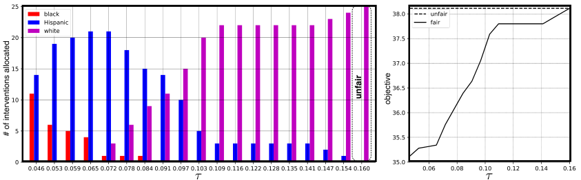
To evaluate the effect on SAT/ACT-taking when intervening on Calculus courses we start with null allocation vector (i.e., no school has a Calculus course). We then solve the optimization problem in eq. (5) with the structural equation for in eq. (7), and a budget of schools. The results of the fair model is shown in Figure 4. The left plot shows the number of interventions allocated to schools by race. The right plot shows the objective value achieved by the fair and unfair (unconstrained) models. On the far right of the left plot is the unfair allocation. In this case, all interventions are given to predominantly white schools. When is small both predominantly black and Hispanic schools receive allocations because these schools benefit the least from their race. As is increased Hispanic school allocations increase, then decrease as white schools are allocated.
Figure 5 shows how each policy allocates interventions on a map of New York City. The fair policy (, the first set of bars in Figure 4) assigns interventions to predominantly Hispanic and black schools that have high utility because of things not due to race. Some of these schools are in neighborhoods with low median income such as North Bronx and North Manhattan66 6 http://uk.businessinsider.com/new-york-city-income-maps-2014-12?r=US&IR=T. As is increased (, the seventh set of bars in Figure 4) the allocation includes more majority white schools, less black schools, and roughly the same number of Hispanic schools. There are more allocations in Brooklyn and Queens. The only intervention to a majority black school kept is to the one in the racially-diverse St. George neighborhood of Staten Island77 7 https://www.nytimes.com/interactive/2015/07/08/us/census-race-map.html. The unfair policy assigns interventions to schools in traditionally white neighborhoods including lower Manhattan, and lower Brooklyn, and all allocations are to white schools. Curiously, many of the interventions made by the unfair model in Manhattan are nearby those made by the fair models to majority Hispanic schools.
5 Conclusion
In this paper we depart from much of the past work on algorithmic fairness by focusing on designing fair interventions to change the underlying system rather than on fair prediction. We make use of structural causal models to encode the effects of public policy interventions, including potential interference. For concreteness we pursued a particular optimization problem where the intervention has a budget constraint, but the approach can be used for other kinds of optimization problems. We devised a fairness criterion that allows us to find beneficial interventions while bounding the benefit to individuals caused by being a member of a privileged group, as determined by the causal model. We test our method on allocating college-preparatory classes to NYC schools fairly. We found that when the fairness criterion holds, interventions are given to a more racially diverse set of schools.
References
- [1] D. Arbour, D. Garant, and D. Jensen. Inferring network effects in relational data. KDD ’16 Proceedings of the 22nd ACM SIGKDD International Conference on Knowledge Discovery and Data Mining, pages 715–724, 2016.
- [2] P. M. Aronow and C. Samii. Estimating average causal effects under general interference, with application to a social network experiment. Annals of Applied Statistics, 11:1912–1947, 2017.
- [3] Chelsea Barabas, Madars Virza, Karthik Dinakar, Joichi Ito, and Jonathan Zittrain. Interventions over predictions: Reframing the ethical debate for actuarial risk assessment. In Sorelle A. Friedler and Christo Wilson, editors, Proceedings of the 1st Conference on Fairness, Accountability and Transparency, volume 81 of Proceedings of Machine Learning Research, pages 62–76, New York, NY, USA, 23–24 Feb 2018. PMLR. URL http://proceedings.mlr.press/v81/barabas18a.html.
- [4] Richard Berk, Hoda Heidari, Shahin Jabbari, Michael Kearns, and Aaron Roth. Fairness in criminal justice risk assessments: The state of the art. arXiv preprint:1703.09207, 2017.
- [5] Tolga Bolukbasi, Kai-Wei Chang, James Y Zou, Venkatesh Saligrama, and Adam T Kalai. Man is to computer programmer as woman is to homemaker? debiasing word embeddings. In Advances in Neural Information Processing Systems, pages 4349–4357, 2016.
- [6] S. Chiappa and T. Gillam. Path-specific counterfactual fairness. arXiv:1802.08139, 2018.
- [7] Alexandra Chouldechova. Fair prediction with disparate impact: A study of bias in recidivism prediction instruments. Big data, 2017.
- [8] A. P. Dawid. Influence diagrams for causal modelling and inference. International Statistical Review, 70:161–189, 2002.
- [9] Cynthia Dwork, Moritz Hardt, Toniann Pitassi, Omer Reingold, and Richard Zemel. Fairness through awareness. In Innovations in Theoretical Computer Science Conference, 2012.
- [10] Cynthia Dwork, Nicole Immorlica, Adam Tauman Kalai, and Mark DM Leiserson. Decoupled classifiers for group-fair and efficient machine learning. In Conference on Fairness, Accountability and Transparency, pages 119–133, 2018.
- [11] T. J. VanderWeele E. L. Ogburn. Causal diagrams for interference. Statistical Science, 29:559–578, 2014.
- [12] Harrison Edwards and Amos Storkey. Censoring representations with an adversary. arXiv preprint:1511.05897, 2015.
- [13] Anthony W Flores, Kristin Bechtel, and Christopher T Lowenkamp. False positives, false negatives, and false analyses: A rejoinder to machine bias: There’s software used across the country to predict future criminals. and it’s biased against blacks. Fed. Probation, 2016.
- [14] Moritz Hardt, Eric Price, Nati Srebro, et al. Equality of opportunity in supervised learning. In Advances in neural information processing systems, 2016.
- [15] Faisal Kamiran and Toon Calders. Classifying without discriminating. In International Conference on Computer, Control and Communication, 2009.
- [16] Toshihiro Kamishima, Shotaro Akaho, Hideki Asoh, and Jun Sakuma. Fairness-aware classifier with prejudice remover regularizer. In Joint European Conference on Machine Learning and Knowledge Discovery in Databases, 2012.
- [17] Niki Kilbertus, Mateo Rojas Carulla, Giambattista Parascandolo, Moritz Hardt, Dominik Janzing, and Bernhard Schölkopf. Avoiding discrimination through causal reasoning. In Advances in Neural Information Processing Systems, 2017.
- [18] Jon Kleinberg, Sendhil Mullainathan, and Manish Raghavan. Inherent trade-offs in the fair determination of risk scores. arXiv preprint:1609.05807, 2016.
- [19] M. Kusner, J. Loftus, C. Russell, and R. Silva. Counterfactual fairness. Advances in Neural Information Processing Systems, 30:4066–4076, 2017.
- [20] Jeff Larson, Surya Mattu, Lauren Kirchner, and Julia Angwin. How we analyzed the compas recidivism algorithm. ProPublica (5 2016), 9, 2016.
- [21] L. T. Liu, S. Dean, E. Rolf, M. Simchowitz, and M. Hardt. Delayed impact of fair machine learning. arXiv:1803.04383, 2018a.
- [22] Lydia T Liu, Sarah Dean, Esther Rolf, Max Simchowitz, and Moritz Hardt. Delayed impact of fair machine learning. arXiv preprint arXiv:1803.04383, 2018b.
- [23] J. Loftus, C. Russell, M. Kusner, and R. Silva. Causal reasoning for algorithmic fairness. arxiv:1805.05859, 2018.
- [24] Razieh Nabi and Ilya Shpitser. Fair inference on outcomes. Thirty-Second AAAI Conference on Artificial Intelligence, 2018.
- [25] J. Pearl. Causality: Models, Reasoning and Inference. Cambridge University Press, 2000.
- [26] J. Pearl, M. Glymour, and N. Jewell. Causal Inference in Statistics: a Primer. Wiley, 2016.
- [27] Gareth William Peters. Statistical machine learning and data analytic methods for risk and insurance. 2017.
- [28] Geoff Pleiss, Manish Raghavan, Felix Wu, Jon Kleinberg, and Kilian Q Weinberger. On fairness and calibration. In Advances in Neural Information Processing Systems, 2017.
- [29] C. Russell, M. Kusner, J. Loftus, and R. Silva. When worlds collide: integrating different counterfactual assumptons in fairness. Advances in Neural Information Processing Systems, 30:6417–6426, 2017.
- [30] M. Sobel. What do randomized studies of housing mobility demonstrate? Journal of the American Statistical Association, 101:1398–1407, 2006.
- [31] P. Spirtes, C. Glymour, and R. Scheines. Causation, Prediction and Search. Lecture Notes in Statistics 81. Springer, 1993.
- [32] Latanya Sweeney. Discrimination in online ad delivery. Queue, 11(3):10, 2013.
- [33] Shuo Yang, Mohammed Korayem, Khalifeh AlJadda, Trey Grainger, and Sriraam Natarajan. Combining content-based and collaborative filtering for job recommendation system: A cost-sensitive statistical relational learning approach. Knowledge-Based Systems, 136:37–45, 2017.
- [34] Muhammad Bilal Zafar, Isabel Valera, Manuel Gomez Rodriguez, and Krishna Gummadi. Fairness beyond disparate treatment & disparate impact: Learning classification without disparate mistreatment. In World Wide Web Conference, 2017.
- [35] Rich Zemel, Yu Wu, Kevin Swersky, Toni Pitassi, and Cynthia Dwork. Learning fair representations. In International Conference on Machine Learning, 2013.
- [36] Jiaming Zeng, Berk Ustun, and Cynthia Rudin. Interpretable classification models for recidivism prediction. Journal of the Royal Statistical Society: Series A (Statistics in Society), 180(3):689–722, 2017.
- [37] Junzhe Zhang and Elias Bareinboim. Fairness in decision-making: The causal explanation formula. In AAAI Conference on Artificial Intelligence, 2018.