Cosmological evolution of the proton-to-electron mass ratio in an extended Brans-Dicke theory
Abstract
We study variation of the proton-to-electron mass ratio by incorporating standard model (SM) of particle physics into an extended Brans-Dicke theory. We show that the evolution of the Higgs vacuum expectation value (VEV), with expansion of the Universe, leads to the variation of the proton-to-electron mass ratio. This is because the electron mass is proportional to the Higgs VEV, while the proton mass is mainly dependent on the quantum chromodynamics (QCD) energy scale, i.e., . Therefore, using the experimental and cosmological constraints on the variation of the we can constrain the variation of the Higgs VEV. This study is important in understanding the recent claims of the detection of a variation of the proton-to-electron mass ratio in quasar absorption spectra.
August 24, 2026
1 Introduction
The assumption of the constancy of the constants plays an important role in astronomy and cosmology, especially with respect to the look-back time measured by the redshift. Refusing the possibility of varying constants could lead to a distorted view of the Universe and, if such a variation were founded, corrections would have to be applied. Therefore, it is important to investigate this possibility, in particular as the measurements become more and more strict. The history of these investigations traces back to early ideas in the 1930s on the possibility of a time variation of the gravitational constant by Milne [1] and the suggestion by Dirac of the large number hypothesis [2, 3] which led him also to propose in 1937 the time evolution of . Clearly, the constants have not undergone enormous variations on solar system scales and geological time scales, and one is looking for tiny effects. There are some reviews on the time variation of the constants of nature, for example see [4, 5, 6, 7].
The proton-to-electron mass ratio is another important dimensionless constant that may evolve with cosmic time. This ratio is effectively the ratio of the strong and electroweak scales. The molecular absorption lines spectra, as first pointed out by Thompson [8], can provide a test of the variation of . The variation of this ratio has been measured using quasar absorption lines [9, 10, 11, 12, 13, 14]. Motivated by these observations of quasar absorption systems, some theories have been proposed, for example see [15, 16, 17, 18, 19, 20, 21, 22]. In this paper, considering the standard model of particle physics and a generalized Brans-Dicke (BD) theory containing two interacting scalar fields, we propose another scenario in which the proton-to-electron mass ratio varies with cosmic time.
According to the standard model of particle physics, the masses of elementary particles, including the electron mass, is proportional to the vacuum expectation value (VEV) of the Higgs boson while the proton mass is mainly determined by the scale of quantum chromodynamics (QCD), i.e., [23]. Therefore, the variation of the Higgs VEV, , leads to a variation of the electron mass while the proton mass almost remains constant (We have also supposed that Yukawa coupling constant between Higgs boson and electron is time-independent). On the other hand, there must be a time, for example the time of electroweak phase transition, when Higgs VEV were different from what is today. Therefore, it is natural to expect that Higgs VEV has been varied during cosmological epochs. Indeed, in the framework of generalized Brans-Dicke (BD) theories, in which BD-field interacts with Higgs field , one can show the effective potential associated to may adopt the Higgs potential form with a slowly evolving vacuum expectation value.
In the next section we discuss the variation of the electron mass and proton mass with the evolution of the Higss VEV. The study of the evolution of the Higgs VEV in cosmological context comes next. Finally, in the conclusion section, using experimental and cosmological observations, we put a constraint on the variation of the Higss VEV.
2 Standard Model and electron/proton mass
The Higgs boson is presumed by the electroweak theory initially to explain the origin of particle masses. In the Standard Model of particle physics, the mass of all elementary particles is proportional to the Higgs VEV. Therefore, for the electron mass as well as the quarks masses, we have
| (1) |
where is the Yukawa coupling and is the Higgs VEV. On the other hand, how the proton mass is related to the Higgs VEV is another question. The total proton mass is 938 MeV, while the masses of the valence quarks in the proton are just 3 MeV per quark which is directly related to the Higgs VEV. The quark and gluon contributions to the proton mass can be provided by solving QCD non-perturbatively. The proton mass is a function of and quark masses. In the chiral limit the theory contains massless physical particles. In this limit is proportional to the QCD energy scale and it does not change with variation of the Higgs VEV. Considering quark masses, the quark mass expansion for the proton mass has the structure [23]
| (2) |
One can derive a separation of the nucleon mass into the contributions from the quark, antiquark, gluon kinetic and potential energies, quark masses, and the trace anomaly [24]. The QCD Hamiltonian can be separated into four gauge-invariant parts
| (3) |
with
| (4) | ||||
| (5) | ||||
| (6) | ||||
| (7) |
where is the quark field, and E and B are electric and magnetic gluon field strengths, respectively. In Eq. (3), represents the quark and antiquark kinetic and potential energies, is the quark mass term, represents the gluon energy, and finally, is the trace anomaly term. Recent lattice simulations shows that the joint u/d/s quark mass term, , only contribute 9 percent of the proton mass [25]. Note that this term is the one where the Higgs boson contributes and it means the second term in Eq. (2) contribute 9 percent of the proton mass. Following [21], we assume that as well as Yukawa couplings are constants, while the Higgs VEV can evolve. Note that it is not the only option. For example in [26] such assumption is not made and nevertheless an alternative scenario changing the proton-to-electron mass ratio is obtained.
According to Eqs. (1) and (2) we have
| (8) | ||||
| (9) |
In Eq. (9), as we discussed before, we have assumed the quark mass term, , contribute 9 percent of the proton mass. Thus is negligible in comparison with and it means, considering time-dependent Higgs VEV, the electron mass should change with the cosmic time while the proton mass remains (almost) constant.
According to Eqs. (8) and (9), the cosmological evolution of the Higgs VEV would lead to a cosmological variation of the proton-to-electron mass ratio :
| (10) |
where for and the present value of the Higgs VEV and its value in the absorption cloud at redshift , respectively.
In order to provide another estimation for as function of , we consider the relation between top quark mass and proton mass discussed in [27]. In [27], using the renormalization group equation, it is argued that in a simple unified theory the proton mass depends on the top quark mass, , as the following
| (11) |
According to this relation, we get
| (12) |
which is in good agreement with Eq. (9).
In the following, we will show how the Higgs VEV, and consequently the proton-to-electron mass ratio, varies with cosmic time.
3 Expansion of the Universe and evolution of the Higgs VEV
Consider the Higgs sector of the standard model (in unitary gauge) with the following Lagrangaian
| (13) |
where is the present Higgs VEV.
One can decompose to the Higgs particle and a classical background field which plays the role of a Higgs cosmological value depending on the cosmic time: . In Lagrangian (13), according to spontaneous symmetry breaking, we should replace with where the time-dependent Higgs vacuum expectation value defined as . Then by minimally coupling to gravity, one can show that the expansion of the Universe leads to a cosmological time evolution of the vacuum expectation of the Higgs boson [21]. Time-dependent Higgs VEV is also studied in [28] considering dynamics of the standard model of particle physics alone. In this work, it has been shown that variation of the Higgs VEV leads to the non-adiabatic production of both bosons and fermions. There are other motivations for time-dependent Higgs VEV as well. For example in [29], the structure of the Higgs potential has been derived from a generalized Brans-Dicke theory [30] containing two interacting scalar fields. By requiring that the cosmological solutions of the model are consistent with observations, it has been shown that the effective scalar field potential adopts the Higgs potential form with a mildly time-dependent Higgs VEV. We conclude that time-dependent Higgs VEV is a natural assumption specially in the context of gravity and cosmology.
Motivated by these arguments, here we assume the Higgs VEV could be time-dependent. However, this does not mean that it certainly varies with time. We just consider it as a well-motivated possibility. Therefore, keeping an open mind on this possibility, we let equations determine the dynamics of its variation. The most stringent bound on comes from the comparison of the transitions in Yb+ with the cesium atomic clock [31]:
| (14) |
Comparing this value with Hubble constant , we obtain an experimental limit . In the end, one can constrain higgs VEV variation using this experimental data and cosmological observations coming from quasar absorption spectra.
In this section, we consider a generalized Brans-Dicke theory containing two interacting scalar fields used in [29]. In this approach, a mildly time-dependent Higgs VEV is derived from evolution of another scalar field. Note that Brans-Dicke theories are connected to the running vacuum models [32, 33]. These models can also produce a change of the vacuum with the expansion of the universe and they are highly competitive in the fitting of the cosmological data, see e.g. [34, 35, 36, 37]
The Universe is isotropic and homogeneous, at least as a first approximation. This assumption will lead us to the Robertson-Walker metric. Almost all of modern cosmology is based on this metric:
| (15) |
where is the curvature signature and is the scale factor. Now consider an extend Brans-Dicke model with the BD-field, , and another scalar field which eventually plays the role of Higgs field. There is a coupling term between these scalar fields, as well as non-minimal interactions with gravity. The new Brans-Dicke model includes all of the terms of the SM, however, we only consider the part of this action containing the dynamics and interaction between the scalar fields, as well as their couplings to gravity. This action is used in [29] in which the authors proposed a physical motivation for the structure of the Higgs potential. The scalar part of the action is:
| (16) |
where is Ricci scalar of curvature, and , , and are dimensionless constants. In action (16), is
| (17) |
which allows generalized derivative couplings of with gravity. The couplings and in (17) were first studied in [38, 39]. So far, the Higgs potential in (16) is unidentified. However, it takes the Higgs potential form after imposing the appropriate conditions.
The Euler-Lagrange equations corresponding to action (16) in the cosmological context with Robertson-Walker metric, Eq. (15), are given by [29]
| (18) |
| (19) |
| (20) |
where is the Hubble parameter.
The above equations can take the power-law solutions:
| (21) |
where and are dimensionless parameters. Since controls the evolution of Newton’s gravitational coupling in the context of BD-model, we expect to be small. Indeed, from observation we know that [5], but its sign is undetermined, see e.g. [40]. Furthermore, consistency of Euler-Lagrange equation (20) with power-law solutions (21) implies .
According to the solution (21), the first three terms of in (18) are proportional to while the other terms are proportional to . Therefore, equation (18) leads to the Higgs-like potential for field
| (22) |
where . Eqs. (19) and (20) lead to two constraints for the parameters of extended BD-action and constants in solution (21), so they are irrelevant in our study. In this approach parameters of Higgs potential (22) are related to the parameters of extended BD-action (16) which can be fixed so that and be positive and take SM values. Actually it is easy to see why should be positive. The sign of would be determined by the BD parameter in the third term of (18) and the cosmological constraint [41], leads to the negative sign in (22)).
Regarding Eq. (22), Higgs VEV is given by
| (23) |
Therefore, the Higgs VEV is depending on the cosmic time.
| (24) |
As we mentioned before, we have an experimental limit . This limit leads to . This constraint is much stronger than what we mentioned before, i.e., . However, this bound strongly depends on our assumption, i.e., constant .
4 Results and Conclusion
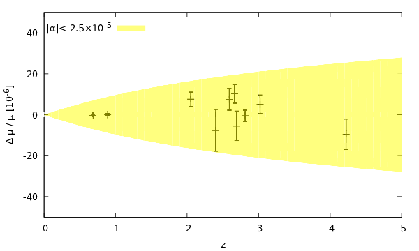
In Fig. 1 variation of the proton-to-electron mass ratio versus redshift has been depicted for . The colored region is compatible with observational data which can be seen in Fig. 1. These data are given in Table 1 in which the weighted average over observational values for eight quasar absorption spectra [42, 43, 44, 45, 46] are taken from [47]). Apart from the spectra for , we also show two observational data of other molecules spectra for [48, 49, 50].
| \topruleQuasar | Redshift | |
|---|---|---|
| B0218+357 | 0.685 | |
| PKS1830-211 | 0.89 | |
| HE0027-1836 | 2.40 | |
| Q0347-383 | 3.02 | |
| Q0405-443 | 2.59 | |
| Q0528-250 | 2.81 | |
| B0642-5038 | 2.66 | |
| J1237+064 | 2.69 | |
| J1443+2724 | 4.22 | |
| J2123-005 | 2.05 | |
| \botrule |
Note that, the Higgs potential itself has been derived from an extended BD-action with a mildly time-dependent Higgs VEV. Our result is compatible with BBN constraint on variation of the Higgs VEV, i.e., [51]. According to Eq. (25), for Gyr and min (with ), we obtain which is compatible with .
The field is also related to the effective gravitational ”constant” in BD theory, , therefore, one can constrain using the constraints on the gravitational constant [5] which, as mentioned before, leads to . On the other hand, observations of quasar absorption spectra, including those listed in Table 1, set a constraint on a varying proton-to-electron mass ratio of holding for redshifts in the range (for a review see [47]). According to Eq. (10) this directly constrains the variation of the Higgs VEV or equivalently the parameter in (24). As it is shown in Fig. 1 we estimate that . Note that this bound depends on our particular model in which we have assumed is NOT running.
Finally, we should mention that environmental conditions, such as the presence of strong gravitational fields [52], can also affect the variation of the proton-to-electron mass ratio, and these effects can distort look-back times effects discussed here.
Acknowledgement
This work is supported financially by the Young Researchers and Elite Club of Islamshahr Branch of Islamic Azad University.
References
- [1] E. A. Milne, Proc. R. Soc. A3 (1937) 242.
- [2] P. A. M. Dirac, The Cosmological constants, Nature 139 (1937) 323.
- [3] P. A. M. Dirac, New basis for cosmology, Proc. Roy. Soc. Lond. A165 (1938) 199.
- [4] J.-P. Uzan, The Fundamental constants and their variation: Observational status and theoretical motivations, Rev. Mod. Phys. 75 (2003) 403 [hep-ph/0205340] [INSPIRE].
- [5] J.-P. Uzan, Varying Constants, Gravitation and Cosmology, Living Rev. Rel. 14 (2011) 2 [arXiv:1009.5514] [INSPIRE].
- [6] T. Chiba, The Constancy of the Constants of Nature: Updates, Prog. Theor. Phys. 126 (2011) 993 [arXiv:1111.0092] [INSPIRE].
- [7] X. Calmet and M. Keller, Cosmological Evolution of Fundamental Constants: From Theory to Experiment, Mod. Phys. Lett. A30 (2015) 1540028 [arXiv:1410.2765] [INSPIRE].
- [8] R. Thompson, Astron. Lett. 16 (1975) 3.
- [9] E. Reinhold, R. Buning, U. Hollenstein, A. Ivanchik, P. Petitjean and W. Ubachs, Indication of a Cosmological Variation of the Proton - Electron Mass Ratio Based on Laboratory Measurement and Reanalysis of H(2) Spectra, Phys. Rev. Lett. 96 (2006) 151101.
- [10] V. V. Flambaum, M. G. Kozlov and M. G. Kozlov, Limit on the Cosmological Variation of mp/me from the Inversion Spectrum of Ammonia, Phys. Rev. Lett. 98 (2007) 240801 [arXiv:0704.2301] [INSPIRE].
- [11] J. A. King, M. T. Murphy, W. Ubachs and J. K. Webb, New constraint on cosmological variation of the proton-to-electron mass ratio from Q0528-250, Mon. Not. Roy. Astron. Soc. 417 (2011) 3010 [arXiv:1106.5786] [INSPIRE].
- [12] J. Bagdonaite, M. T. Murphy, L. Kaper and W. Ubachs, Constraint on a variation of the proton-to-electron mass ratio from H2 absorption towards quasar Q2348-011, Mon. Not. Roy. Astron. Soc. 421 (2012) 419 [arXiv:1112.0428] [INSPIRE].
- [13] H. Rahmani et al., The UVES Large Program for Testing Fundamental Physics II: Constraints on a Change in Towards Quasar HE 0027-1836, Mon. Not. Roy. Astron. Soc. 435 (2013) 861 [arXiv:1307.5864] [INSPIRE].
- [14] M. Dapra, P. Noterdaeme, M. Vonk, M. T. Murphy and W. Ubachs, Analysis of carbon monoxide absorption at zabs 2.5 to constrain variation of the proton-to-electron mass ratio, Mon. Not. Roy. Astron. Soc. 467 (2017) 3848 [arXiv:1702.03132] [INSPIRE].
- [15] J. D. Barrow and J. Magueijo, Cosmological constraints on a dynamical electron mass, Phys. Rev. D72 (2005) 043521 [astro-ph/0503222] [INSPIRE].
- [16] X. Calmet and H. Fritzsch, A Time Variation of Proton-Electron Mass Ratio and Grand Unification, Europhys. Lett. 76 (2006) 1064 [astro-ph/0605232] [INSPIRE].
- [17] T. Dent, Composition-dependent long range forces from varying m(p)/m(e), JCAP 0701 (2007) 013 [hep-ph/0608067] [INSPIRE].
- [18] T. Chiba, T. Kobayashi, M. Yamaguchi and J. Yokoyama, Time variation of proton-electron mass ratio and fine structure constant with runaway dilaton, Phys. Rev. D75 (2007) 043516 [hep-ph/0610027] [INSPIRE].
- [19] S. Lee, Time Variation of Fine Structure Constant and Proton-Electron Mass Ratio with Quintessence, Mod. Phys. Lett. A22 (2007) 2003 [astro-ph/0702063] [INSPIRE].
- [20] P. P. Avelino, On the cosmological evolution of alpha and mu and the dynamics of dark energy, Phys. Rev. D78 (2008) 043516 [arXiv:0804.3394] [INSPIRE].
- [21] X. Calmet, Cosmological evolution of the Higgs boson’s vacuum expectation value, Eur. Phys. J. C77 (2017) 729 [arXiv:1707.06922] [INSPIRE].
- [22] H. Fritzsch, J. Solà Peracaula and R. C. Nunes, Running vacuum in the Universe and the time variation of the fundamental constants of Nature, Eur. Phys. J. C77 (2017) 193 [arXiv:1605.06104] [INSPIRE].
- [23] J. Gasser and H. Leutwyler, Quark Masses, Phys. Rept. 87 (1982) 77.
- [24] X.-D. Ji, A QCD analysis of the mass structure of the nucleon, Phys. Rev. Lett. 74 (1995) 1071 [hep-ph/9410274] [INSPIRE].
- [25] Y.-B. Yang, J. Liang, Y.-J. Bi, Y. Chen, T. Draper, K.-F. Liu et al., Proton Mass Decomposition from the QCD Energy Momentum Tensor, Phys. Rev. Lett. 121 (2018) 212001 [arXiv:1808.08677] [INSPIRE].
- [26] H. Fritzsch and J. Solà Peracaula, Matter Non-conservation in the Universe and Dynamical Dark Energy, Class. Quant. Grav. 29 (2012) 215002 [arXiv:1202.5097] [INSPIRE].
- [27] C. Quigg, Hadron colliders, the top quark, and the Higgs sector, in Electroweak theory. Proceedings, Advanced School, Mao, Spain, June 16-22, 1996, pp. 115–177, 1996, hep-ph/9707508 [INSPIRE]
- [28] R. Casadio, P. L. Iafelice and G. P. Vacca, Non-adiabatic quantum effects from a Standard Model time-dependent Higgs vev, Nucl. Phys. B783 (2007) 1 [hep-th/0702175] [INSPIRE].
- [29] J. Solà Peracaula, E. Karimkhani and A. Khodam-Mohammadi, Higgs potential from extended Brans-Dicke theory and the time-evolution of the fundamental constants, Class. Quant. Grav. 34 (2017) 025006 [arXiv:1609.00350] [INSPIRE].
- [30] C. Brans and R. H. Dicke, Mach’s principle and a relativistic theory of gravitation, Phys. Rev. 124 (1961) 925.
- [31] N. Huntemann, B. Lipphardt, C. Tamm, V. Gerginov, S. Weyers and E. Peik, Improved limit on a temporal variation of from comparisons of Yb+ and Cs atomic clocks, Phys. Rev. Lett. 113 (2014) 210802 [arXiv:1407.4408] [INSPIRE].
- [32] J. Solà Peracaula, Brans-Dicke gravity: From Higgs physics to (dynamical) dark energy, Int. J. Mod. Phys. D27 (2018) 1847029 [arXiv:1805.09810] [INSPIRE].
- [33] J. de Cruz Pérez and J. Solà Peracaula, Brans-Dicke cosmology mimicking running vacuum, Mod. Phys. Lett. A33 (2018) 1850228 [arXiv:1809.03329] [INSPIRE].
- [34] A. Gómez-Valent and J. Solà Peracaula, Density perturbations for running vacuum: a successful approach to structure formation and to the -tension, Mon. Not. Roy. Astron. Soc. 478 (2018) 126 [arXiv:1801.08501] [INSPIRE].
- [35] J. Solà Peracaula, J. d. C. Perez and A. Gomez-Valent, Possible signals of vacuum dynamics in the Universe, Mon. Not. Roy. Astron. Soc. 478 (2018) 4357 [arXiv:1703.08218] [INSPIRE].
- [36] J. Solà Peracaula, J. de Cruz Pérez and A. Gómez-Valent, Dynamical dark energy vs. = const in light of observations, EPL 121 (2018) 39001 [arXiv:1606.00450] [INSPIRE].
- [37] J. Solà Peracaula, A. Gómez-Valent and J. de Cruz Pérez, First evidence of running cosmic vacuum: challenging the concordance model, Astrophys. J. 836 (2017) 43 [arXiv:1602.02103] [INSPIRE].
- [38] L. Amendola, Cosmology with nonminimal derivative couplings, Phys. Lett. B301 (1993) 175 [gr-qc/9302010] [INSPIRE].
- [39] S. Capozziello and G. Lambiase, Nonminimal derivative coupling and the recovering of cosmological constant, Gen. Rel. Grav. 31 (1999) 1005 [gr-qc/9901051] [INSPIRE].
- [40] Y.-C. Li, F.-Q. Wu and X. Chen, Constraints on the Brans-Dicke gravity theory with the Planck data, Phys. Rev. D88 (2013) 084053 [arXiv:1305.0055] [INSPIRE].
- [41] A. Avilez and C. Skordis, Cosmological constraints on Brans-Dicke theory, Phys. Rev. Lett. 113 (2014) 011101 [arXiv:1303.4330] [INSPIRE].
- [42] J. A. King, J. K. Webb, M. T. Murphy and R. F. Carswell, Stringent null constraint on cosmological evolution of the proton-to-electron mass ratio, Phys. Rev. Lett. 101 (2008) 251304 [arXiv:0807.4366] [INSPIRE].
- [43] A. L. Malec, R. Buning, M. T. Murphy, N. Milutinovic, S. L. Ellison, J. X. Prochaska et al., Keck Telescope Constraint on Cosmological Variation of the Proton-to-Electron Mass Ratio, Mon. Not. Roy. Astron. Soc. 403 (2010) 1541 [arXiv:1001.4078] [INSPIRE].
- [44] F. van Weerdenburg, M. T. Murphy, A. L. Malec, L. Kaper and W. Ubachs, First constraint on cosmological variation of the proton-to-electron mass ratio from two independent telescopes, Phys. Rev. Lett. 106 (2011) 180802 [arXiv:1104.2969] [INSPIRE].
- [45] M. Wendt and P. Molaro, Robust limit on a varying proton-to-electron mass ratio from a single H2 system, Astron. Astrophys. 526 (2011) A96 [arXiv:1009.3133] [INSPIRE].
- [46] M. Dapra, M. van der Laan, M. T. Murphy and W. Ubachs, Constraint on a varying proton-to-electron mass ratio from H2 and HD absorption at zabs 2.34, Mon. Not. Roy. Astron. Soc. 465 (2017) 4057 [arXiv:1611.05191] [INSPIRE].
- [47] W. Ubachs, J. Bagdonaite, E. J. Salumbides, M. T. Murphy and L. Kaper, Search for a drifting proton–electron mass ratio from H2, Rev. Mod. Phys. 88 (2016) 021003 [arXiv:1511.04476] [INSPIRE].
- [48] M. T. Murphy, V. V. Flambaum, S. Muller and C. Henkel, Strong Limit on a Variable Proton-to-Electron Mass Ratio from Molecules in the Distant Universe, Science 320 (2008) 1611 [arXiv:0806.3081] [INSPIRE].
- [49] N. Kanekar, Constraining changes in the proton-electron mass ratio with inversion and rotational lines, Astrophys. J. 728 (2011) L12 [arXiv:1101.4029] [INSPIRE].
- [50] C. Henkel, K. M. Menten, M. T. Murphy, N. Jethava, V. V. Flambaum, J. A. Braatz et al., The density, the cosmic microwave background, and the proton-to-electron mass ratio in a cloud at redshift 0.9, Astron. Astrophys. 500 (2009) 725 [arXiv:0904.3081] [INSPIRE].
- [51] J. Yoo and R. J. Scherrer, Big bang nucleosynthesis and cosmic microwave background constraints on the time variation of the Higgs vacuum expectation value, Phys. Rev. D67 (2003) 043517 [astro-ph/0211545] [INSPIRE].
- [52] J. Bagdonaite, E. J. Salumbides, S. P. Preval, M. A. Barstow, J. D. Barrow, M. T. Murphy et al., Limits on a Gravitational Field Dependence of the Proton-Electron Mass Ratio from H2 in White Dwarf Stars, Phys. Rev. Lett. 113 (2014) 123002 [arXiv:1409.1000] [INSPIRE].