merlin - a unified modelling framework for data analysis and methods development in Stata

University of Leicester

michael.crowther@le.ac.uk

Abstract

merlin can do a lot of things. From simple stuff, like fitting a linear regression or a Weibull survival model, to a three-level logistic mixed effects model, or a multivariate joint model of multiple longitudinal outcomes (of different types) and a recurrent event and survival with non-linear effects…the list is rather endless. merlin can do things I haven’t even thought of yet. I’ll take a single dataset, and attempt to show you the full range of capabilities of merlin, and discuss some future directions for the implementation in Stata.

Draft v1: August 24, 2026

1 Introduction

gsem’s introduction in Stata 14 brought an extremely broad class of mixed effects models (among other things), and most importantly (from my perspective), is that gsem is fast. gsem has full analytic derivatives for any model that you fit, including a model with any number of levels and random effects at each level. Of course, gllamm came along before gsem, providing a very flexible framework in Stata for modelling data (Rabe-Hesketh et al., 2002; Rabe-Hesketh et al., 2005). But inevitably, every program is limited to certain families of distributions, and complexity of the linear predictors, and of course computational speed.

Much of my previous work has centred on joint longitudinal-survival analysis, implemented in the stjm command (Crowther et al., 2013), which can fit a joint model for a continuous, repeatedly measured biomarker, and a single time-to-event. There is flexibility, in that you can use splines or polynomials to model the biomarker over time, and there’s lots of choices for your survival model, including spline based approaches. The main benefit of stjm is the added flexibility in how to link the two submodels, through things like the expected value, or derivatives of it, which are commonly used in the joint model literature. Given this starting point, the natural extension is to allow for more than one biomarker, recurrent events, competing risks…the list goes on. I’ve also released stmixed in Stata (Crowther et al., 2014), for two-level parametric survival models, in particular for the Royston-Parmar spline based model, and stgenreg for general hazard based regression (Crowther and Lambert, 2013; Crowther and Lambert, 2014), where the user could specify their own functional form for the hazard function, and stgenreg would use numerical quadrature to maximise the likelihood.

The aim of merlin was to bring together my previous programs, but also provide a whole lot more. In this paper, I’ll introduce the core features and syntax of merlin and illustrate a variety of models that can be fitted with it. More details on the methodological framework can be found in Crowther (2017). The paper is structured as follows: In Section 2 I describe the top level syntax of the merlin command and describe many of the options, and in Section 3 I detail some examples, showing the wide variety of available models. I conclude the paper in Section 4 with a discussion of merlin and its potential.

2 The architecture of merlin

merlin is designed to be as flexible and general as possible. There is no real limit to what it can do, given that the user can readily extend it. You can specify any number of outcome models, which can be linked in any number of ways. Each outcome model, $i=1,\dots,M$ , has a main complex predictor (you can have more, but I’ll leave that to another time), which is made up of additive components, $c=1,\dots,C$ , where each component is made up of multiplicative elements, $e=1,\dots,E$ .

g_{i}(\mu_{i}(y_{i}|x,b))=\sum_{c=1}^{C}\prod_{e=1}^{E}\psi_{ice}(x,b)

where for the $i^{th}$ model, $y_{i}$ is the observed response, $x$ is the full design matrix, and $b$ are the stacked multivariate normal or $t$ -distributed random effects. We have link function, $g_{i}()$ , and expected value $\mu_{i}$ . $\psi()$ defines essentially an arbitrary function, of which some special cases are defined in the next section.

merlin is estimated using maximum likelihood, with any random effects integrated out using either adaptive or non-adaptive Gaussian quadrature, or Monte Carlo integration. More details on the formulation of the likelihood can be found in Crowther (2017).

2.1 merlin syntax

merlin (model1) [(model2)] [...] [,options]

where the syntax of a modeli is

[depvar] [component1] [component2] [...] [,model_options]

where the syntax of a componentj is

element1[#element2][#element3][...][@real]

and each elementk can take one of the forms described in the next section. At the end of each component, you may optionally specify a constraint on the parameter(s) of the associated component, through use of the @.

model_options include:

•

family(fam,fam_options), where fam can be one of:
- –
  
  gaussian - Gaussian distribution
- –
  
  bernoulli - Bernoulli distribution
- –
  
  beta - beta distribution
- –
  
  poisson - Poisson distribution
- –
  
  ologit - ordinal with logistic link
- –
  
  oprobit - ordinal with probit link
- –
  
  exponential - exponential distribution
- –
  
  weibull - Weibull distribution
- –
  
  gompertz - Gompertz distribution
- –
  
  gamma - gamma distribution
- –
  
  rp - Royston-Parmar model (restricted cubic spline on log cumulative hazard scale)
- –
  
  rcs - restricted cubic splines on log hazard scale
- –
  
  user - specify your own distribution
  and fam_options include:
- –
  
  failure(varname) - event indicator for a survival model
- –
  
  ltruncated(varname) - left-truncation/delayed entry times for survival model
- –
  
  llfunction(func_name) - name of a Mata function which returns your user-defined log-likelihood contribution
- –
  
  hazard(func_name) - name of a Mata function which returns your user-defined hazard function
- –
  
  chazard(func_name) - name of a Mata function which returns your user-defined cumulative hazard function
- –
  
  nap(#) - estimate # ancillary parameters, which may be called in user-defined functions
•

timevar(varname) - specifies the variable which contains time; this is required to specify time-dependent effects. Generally within a survival model, time must be explicitly handled by merlin. timevar() will be matched against any elements (see the next section) which may use it, to make sure it is handled correctly.

There are many other suboptions available in merlin, which are fully documented in the help files.

2.1.1 Element types

One of the fundamental flexibilities of merlin is the variety of elements that can be used within your model.

•

varname - an independent variable in your dataset
•

rcs(varname ,opts) - a restricted cubic spline function
- –
  
  df(#) - degrees of freedom (# of internal knots + 1). Knots are placed at evenly spaced centiles of varname, with boundary knots assumed to be the minimum and maximum of varname.
- –
  
  knots(numlist) - specifies the knots, including the boundary knots.
- –
  
  log - create splines of log(varname) instead of the default untransformed varname
- –
  
  orthog - apply Gram-Schmidt orthogonalisation; can improve convergence
- –
  
  event - used in conjunction with df(), specifies that internal knot locations are based on centiles of only observations of varname that experienced the survival event specified in failure()
- –
  
  offset(varname) - specifies an offset, to be added to varname before the fp() function is built
•

bs(varname ,opts) - a B-spline function
- –
  
  df(#) - specifies the degrees of freedom (not strictly speaking) for the spline function, which allows you to specify internal knots at equally spaced centiles, instead of using knots(). df() is consistent with rcs() elements in how internal knots are chosen.
- –
  
  knots(numlist) - specifies the internal knots, must be in ascending order.
- –
  
  bknots(numlist) - specifies the lower and upper boundary knot locations. Must be in ascending order. Default is the minimum and maximum of varname.
- –
  
  intercept - includes the intercept basis function, which by default is not included.
- –
  
  log - create splines of log(varname) instead of the default untransformed varname
- –
  
  event - used in conjunction with df(), specifies that internal knot locations are based on centiles of only observations of varname that experienced the survival event specified in failure()
- –
  
  offset(varname) - specifies an offset, to be added to varname before the fp() function is built
•

fp(varname ,opts) - a fractional polynomial function (of order 1 or 2), where opts include:
- –
  
  powers(numlist) - powers up to a second-degree FP function, each of which can be one of (-2,-1,-0.5,0,0.5,1,2,3)
- –
  
  offset(varname) - specifies an offset, to be added to varname before the fp() function is built
•

mf(func_name) - a user-defined Mata function (see the section on utility functions)
•

M#[cluster level] - a random effect, defined at the cluster level, for example, M1[centre] defines a random intercept at the centre level, and M2[centre>id] defines a random intercept at the id level.
•

EV[depvar/#] - the expected value of an outcome model
•

dEV[depvar/#] - the first derivative with respect to time of the expected value of an outcome model
•

d2EV[depvar/#] - the second derivative with respect to time of the expected value of an outcome model
•

iEV[depvar/#] - the integral with respect to time of the expected value of an outcome model
•

XB[depvar/#] - the expected value of a complex predictor
•

dXB[depvar/#] - the first derivative with respect to time of the expected value of a complex predictor
•

d2XB[depvar/#] - the second derivative with respect to time of the expected value of a complex predictor
•

iXB[depvar/#] - the integral with respect to time of the expected value of a complex predictor

2.1.2 Utility functions

On one hand, merlin is an engine to estimate many standard models, such as multivariate hierarchical models. On the other, it’s a platform on which to extend and build on. One of the main design features of merlin is the ease at which it can be extended and added to by the user. This makes it extremely useful for methodological research. Utility functions can be used in two main settings.

1.

family(user) - when passing your own log-likelihood function, or hazard and/or cumulative hazard function, utility functions can be used within the Mata function to provide access to anything you may need from the merlin model object
2.

mf() - when specifying your own element type, you can also call any of the utility functions

Available utility functions include:

•

merlin_util_depvar(M) - returns the dependent variable for the current model. This will be a matrix with two columns if failure() is specified, and three columns if ltruncated() has been specified.
•

merlin_util_xzb(M , | real colvector t) - returns the complex predictor for the current model, optionally evaluated at time points t
•

merlin_util_xzb_deriv(M , | real colvector t) - returns d/dt of the complex predictor for the current model, optionally evaluated at time points t
•

merlin_util_xzb_deriv2(M , | real colvector t) - returns d2/dt2 of the complex predictor for the current model, optionally evaluated at time points t
•

merlin_util_xzb_integ(M , | real colvector t) - returns the integral with respect to time of the complex predictor for the current model, optionally evaluated at time points t
•

merlin_util_expval(M , | real colvector t) - returns the expected value of the response for the current model, optionally evaluated at time points t
•

merlin_util_expval_deriv(M , | real colvector t) - returns d/dt of the expected value of the response for the current model, optionally evaluated at time points t
•

merlin_util_expval_deriv2(M , | real colvector t) - returns d2/dt2 of the expected value of the response for the current model, optionally evaluated at time points t
•

merlin_util_expval_integ(M , | real colvector t) - returns the integral of the expected value of the response for the current model, optionally evaluated at time points t
•

merlin_util_ap(M,#)- returns the #th ancillary parameter of the current model
•

merlin_util_timevar(M) - returns the time variable for the current model, which would’ve been specified using the timevar(varname) option

All of the utility function take as their first argument a transmorphic object, in this case I have called it M, but you may call it anything you like. This contains the merlin object, which should not be edited. All of the xzb or expval utility functions have an equivalent *_mod() function, which allows you to specify an additional argument, representing the model which you want to call, e.g. merlin_util_xzb_mod(M,2) will return the complex predictor for the second model in your merlin statement. This can be included in your function for the first, letting you link submodels.

2.1.3 merlin postestimation

merlin comes with a set of post-estimation tools available through the predict function, with the standard syntax of:

predict newvarname, statistic [options]

where statistic includes:

•

mu - expected value of the response
•

eta - expected value of the complex predictor
•

hazard - hazard function
•

chazard - cumulative hazard function
•

survival - survival function
•

cif - cumulative incidence function
•

rmst - restricted mean survival time (integral of survival)
•

timelost - time lost due to the event (integral of cif)

and options include:

•

outcome(#) - specifies the model to predict for; default is outcome(1)
•

fixedonly - calculate prediction based only on the fixed effects
•

marginal - calculate prediction integrating out all random effects, i.e. the population-averaged prediction
•

at(at_spec) - specify covariate patterns at which to calculate the statistic at, e.g. at(trt 1 age 54)
•

timevar(varname) - specify a variable which contains timepoints at which to calculate the statistic at
•

ci - calculate confidence intervals, using the delta method through predictnl
•

causes(numlist) - specifies which models contribute to the calculation; for use in competing risks models

3 Examples

Given how varied and arguably complex the syntax can appear, the easiest way to get to grips with merlin is through some examples. Throughout this section I will use a single dataset (Murtaugh et al., 1994). It’s a commonly used dataset from the joint longitudinal-survival literature, and will serve to illustrate many different analysis techniques, culminating in a detailed, complex multivariate hierarchical model. First I load the data, which you can get from my website,

use "https://www.mjcrowther.co.uk/data/jm_example.dta", clear

The dataset consists of information on 312 patients with primary biliary cirrhosis, of which 140 died during a maximum follow-up of 14.3 years. Covariates of interest include serum bilirubin and prothrombin index, both markers of liver performance, and treatment allocation, trt. Patients were randomised to either D-penicillamine or a placebo. In all analyses, I will work with the log of serum bilirubin, stored in logb. The data structure looks as follows:

. list id stime died trt logb pro time if inlist(id,1,2), sepby(id) noobs

  +------------------------------------------------------------------+
  | id     stime   died         trt        logb   prothr~n      time |
  |------------------------------------------------------------------|
  |  1   1.09517      1   D-penicil    2.674149       12.2         0 |
  |  1         .      .   D-penicil    3.058707       11.2   .525682 |
  |------------------------------------------------------------------|
  |  2   14.1523      0   D-penicil    .0953102       10.6         0 |
  |  2         .      .   D-penicil   -.2231435         11   .498302 |
  |  2         .      .   D-penicil           0       11.6   .999343 |
  |  2         .      .   D-penicil    .6418539       10.6   2.10273 |
  |  2         .      .   D-penicil    .9555114       11.3   4.90089 |
  |  2         .      .   D-penicil    1.280934       11.5   5.88928 |
  |  2         .      .   D-penicil    1.435084       11.5   6.88588 |
  |  2         .      .   D-penicil    1.280934       11.5    7.8907 |
  |  2         .      .   D-penicil    1.526056       11.5   8.83255 |
  +------------------------------------------------------------------+

merlin, just like gsem, treats models in wide format, but observations within a model in long format. Hence, our survival outcome variables, stime and died, must only have one observation per id. If a patient had more than one row of data for their survival outcome, then we could fit a recurrent event model…but that’s a tangent for another time. Speaking of time, our time variable records the times at which the biomarkers logb and prothrombin were recorded.

3.1 Linear mixed effects regression

I will start with a very simple model, a linear regression of logb against time, assuming a Gaussian response:

. merlin (logb time, family(gaussian))

Fitting full model:

Iteration 0:   log likelihood = -3339.4091
Iteration 1:   log likelihood = -3044.5062
Iteration 2:   log likelihood = -2962.0949
Iteration 3:   log likelihood = -2961.4148
Iteration 4:   log likelihood = -2961.4144
Iteration 5:   log likelihood = -2961.4144

Mixed effects regression model                  Number of obs     =      1,945
Log likelihood = -2961.4144
------------------------------------------------------------------------------
             |      Coef.   Std. Err.      z    P>|z|     [95% Conf. Interval]
-------------+----------------------------------------------------------------
logb:        |
        time |   .0139443   .0081287     1.72   0.086    -.0019876    .0298763
       _cons |   .5594103   .0358095    15.62   0.000      .489225    .6295956
  sd(resid.) |   1.109201   .0177842                      1.074886    1.144611
------------------------------------------------------------------------------

Let’s add some flexibility by using the rcs() element, which lets us model the change over time flexibly using restricted cubic splines with three degrees of freedom, i.e. three spline terms.

. merlin (logb rcs(time, df(3)), family(gaussian)), nolog
variables created for model 1, component 1: _cmp_1_1_1 to _cmp_1_1_3

Fitting full model:

Mixed effects regression model                  Number of obs     =      1,945
Log likelihood = -2960.7317
------------------------------------------------------------------------------
             |      Coef.   Std. Err.      z    P>|z|     [95% Conf. Interval]
-------------+----------------------------------------------------------------
logb:        |
     rcs():1 |   .0636201    .065479     0.97   0.331    -.0647164    .1919567
     rcs():2 |   .0057442   .0115642     0.50   0.619    -.0169212    .0284096
     rcs():3 |  -.0012839   .0034269    -0.37   0.708    -.0080005    .0054327
       _cons |    .518356   .0540793     9.59   0.000     .4123626    .6243494
  sd(resid.) |   1.108811    .017778                      1.074509    1.144209
------------------------------------------------------------------------------

If you prefer fractional polynomials or B-splines, then use the fp() or bs() element types. Given our observations are clustered within individuals, let’s add a random intercept:

. merlin (logb rcs(time, df(3)) M1[id]@1, family(gaussian)), nolog
variables created for model 1, component 1: _cmp_1_1_1 to _cmp_1_1_3

Fitting fixed effects model:

Fitting full model:

Mixed effects regression model                  Number of obs     =      1,945
Log likelihood = -1871.1924
------------------------------------------------------------------------------
             |      Coef.   Std. Err.      z    P>|z|     [95% Conf. Interval]
-------------+----------------------------------------------------------------
logb:        |
     rcs():1 |   .1157301   .0300614     3.85   0.000     .0568108    .1746494
     rcs():2 |  -.0047585   .0052904    -0.90   0.368    -.0151275    .0056104
     rcs():3 |   .0024164   .0015696     1.54   0.124    -.0006599    .0054928
      M1[id] |          1          .        .       .            .           .
       _cons |   .5311768   .0666663     7.97   0.000     .4005132    .6618403
  sd(resid.) |   .4866347   .0085298                      .4702005    .5036433
-------------+----------------------------------------------------------------
id:          |
      sd(M1) |   1.099119   .0466923                       1.01131    1.194552
------------------------------------------------------------------------------

I have added M1[id]@1 to my complex predictor. This defines a single normally distributed random effect, called M1, defined at the id level. By default, any component within the complex predictor will have an estimated coefficient. Given our model will already estimate a fixed intercept, we want to constrain the random effects coefficient to be 1, by specifying @1 at the end. Let’s add a random linear slope, and also orthogonalise my spline terms:

. merlin (logb rcs(time, df(3) orthog) time#M2[id]@1 M1[id]@1, family(gaussian)), nolog
variables created for model 1, component 1: _cmp_1_1_1 to _cmp_1_1_3

Fitting fixed effects model:

Fitting full model:

Mixed effects regression model                  Number of obs     =      1,945
Log likelihood = -1531.5158
------------------------------------------------------------------------------
             |      Coef.   Std. Err.      z    P>|z|     [95% Conf. Interval]
-------------+----------------------------------------------------------------
logb:        |
     rcs():1 |   .5469075   .0439678    12.44   0.000     .4607322    .6330827
     rcs():2 |  -.0364925   .0115305    -3.16   0.002    -.0590918   -.0138932
     rcs():3 |   .0115627   .0091666     1.26   0.207    -.0064034    .0295289
 time#M2[id] |          1          .        .       .            .           .
      M1[id] |          1          .        .       .            .           .
       _cons |   1.034689   .0702843    14.72   0.000     .8969347    1.172444
  sd(resid.) |   .3445818   .0066951                      .3317063     .357957
-------------+----------------------------------------------------------------
id:          |
      sd(M1) |   1.011593   .0428349                      .9310276     1.09913
      sd(M2) |   .1814674   .0127782                      .1580739    .2083228
------------------------------------------------------------------------------

Note by orthogonalising the splines, it changes the interpretation of the intercept. I now have a component with more than one element, time#M2[id]@1 - a variable time has been interacted with a random effect called M2 defined at the id level, with its coefficient constrained to be 1. If I’d called it M1 again, then there would only be a single random effect in my model, but used twice, which would not be sensible in this case. By default, each level’s random effects are assumed to have covariance(diagonal). We can relax this by estimating a correlation:

. merlin (logb rcs(time, df(3) orthog) time#M2[id]@1 M1[id]@1, family(gaussian)),  ///
>                                       covariance(unstructured) nolog
variables created for model 1, component 1: _cmp_1_1_1 to _cmp_1_1_3

Fitting fixed effects model:

Fitting full model:

Mixed effects regression model                  Number of obs     =      1,945
Log likelihood =  -1518.484
------------------------------------------------------------------------------
             |      Coef.   Std. Err.      z    P>|z|     [95% Conf. Interval]
-------------+----------------------------------------------------------------
logb:        |
     rcs():1 |   .5975687    .044098    13.55   0.000     .5111382    .6839992
     rcs():2 |  -.0377092    .011405    -3.31   0.001    -.0600625   -.0153559
     rcs():3 |     .01592   .0091416     1.74   0.082    -.0019973    .0338372
 time#M2[id] |          1          .        .       .            .           .
      M1[id] |          1          .        .       .            .           .
       _cons |   1.079191   .0798641    13.51   0.000     .9226599    1.235721
  sd(resid.) |   .3456885   .0067258                      .3327544    .3591254
-------------+----------------------------------------------------------------
id:          |
      sd(M1) |   .9858939   .0421404                      .9066653    1.072046
      sd(M2) |   .1819288   .0127223                      .1586269    .2086537
 corr(M2,M1) |   .4340876   .0739756                       .278697    .5673296
------------------------------------------------------------------------------

which shows evidence of positive correlation between intercept and slope.

3.2 User-defined model

Now I’m going to show you how to replicate the previous model using your own log likelihood function. You simply write your function in Mata, which returns a real matrix containing the observation level log likelihood contribution. This is the code for a Gaussian distributed repsonse:

mata:
real matrix logl(M)
{
    y     = merlin_util_depvar(M)     //extract the response
    xb    = merlin_util_xzb(M)        //get the complex predictor
    sdre  = exp(merlin_util_ap(M,1))  //get the ancillary residual error std. dev.
    logl  = lnnormalden(y,xb,sdre)    //calculate ob. level log likelihood
    return(logl)                      //return result
}
end

I get my dependent variable, my linear predictor, my one ancillary parameter for the residual standard deviation (estimated on the log scale), and use Mata’s internal log normal density function. Now I simply pass it to merlin as a family(user), specifying nap(1) for my residual standard deviation, and you can specify anything you like in the complex predictor. Let’s fit the previous model,

. merlin (logb rcs(time, df(3) orthog) time#M2[id]@1 M1[id]@1,            ///
>                               family(user, llfunction(logl) nap(1))),   ///
>                               covariance(unstructured) nolog
variables created for model 1, component 1: _cmp_1_1_1 to _cmp_1_1_3

Fitting fixed effects model:

Fitting full model:

Mixed effects regression model                  Number of obs     =      1,945
Log likelihood =  -1518.484
------------------------------------------------------------------------------
             |      Coef.   Std. Err.      z    P>|z|     [95% Conf. Interval]
-------------+----------------------------------------------------------------
logb:        |
     rcs():1 |   .5975687    .044098    13.55   0.000     .5111382    .6839992
     rcs():2 |  -.0377092    .011405    -3.31   0.001    -.0600625   -.0153559
     rcs():3 |     .01592   .0091416     1.74   0.082    -.0019973    .0338372
 time#M2[id] |          1          .        .       .            .           .
      M1[id] |          1          .        .       .            .           .
       _cons |   1.079191   .0798641    13.51   0.000     .9226599    1.235721
        ap:1 |  -1.062217   .0194562   -54.60   0.000    -1.100351   -1.024084
-------------+----------------------------------------------------------------
id:          |
      sd(M1) |   .9858939   .0421404                      .9066653    1.072046
      sd(M2) |   .1819288   .0127223                      .1586269    .2086537
 corr(M2,M1) |   .4340876   .0739756                       .278697    .5673296
------------------------------------------------------------------------------

which gives us identical results, as expected. The potential of this sort of implementation is huge.

3.3 Survival/time-to-event analysis

Many standard time-to-event models are available in merlin, including most of those in streg, and some more flexible distributions are also inbuilt. This includes the Royston-Parmar model, and a log hazard scale equivalent model, both using restricted cubic splines to model the baseline. To fit a survival model with merlin, we simply add the failure(varname) option, to specify the event indicator.

3.3.1 Weibull proportional hazards model

Let’s start with a simple Weibull proportional hazards model, adjusting for treatment:

. merlin (stime trt, family(weibull, failure(died)))

Fitting full model:

Iteration 0:   log likelihood = -2000.3067
Iteration 1:   log likelihood = -512.23492
Iteration 2:   log likelihood = -511.85192
Iteration 3:   log likelihood = -511.84742
Iteration 4:   log likelihood = -511.84742

Mixed effects regression model                  Number of obs     =        312
Log likelihood = -511.84742
------------------------------------------------------------------------------
             |      Coef.   Std. Err.      z    P>|z|     [95% Conf. Interval]
-------------+----------------------------------------------------------------
stime:       |
         trt |  -.0004536    .169053    -0.00   0.998    -.3317914    .3308841
       _cons |  -2.815926   .2054485   -13.71   0.000    -3.218597   -2.413254
  log(gamma) |   .0740757   .0752114     0.98   0.325    -.0733359    .2214873
------------------------------------------------------------------------------

Simple, yet effective. Let’s explore some non-standard models.

3.3.2 Spline-based survival model

The Royston-Parmar model is now widely used, using restricted cubic splines to model the baseline log cumulative hazard function, and any time-dependent effects:

. merlin (stime trt, family(rp, failure(died) df(3)))
variables created: _rcs1_1 to _rcs1_3

Fitting full model:

Iteration 0:   log likelihood = -488.26676
Iteration 1:   log likelihood = -356.60857
Iteration 2:   log likelihood = -354.86415
Iteration 3:   log likelihood = -354.85331
Iteration 4:   log likelihood = -354.85331

Mixed effects regression model                  Number of obs     =        312
Log likelihood = -354.85331
------------------------------------------------------------------------------
             |      Coef.   Std. Err.      z    P>|z|     [95% Conf. Interval]
-------------+----------------------------------------------------------------
stime:       |
         trt |   .0001164   .1690663     0.00   0.999    -.3312475    .3314803
       _cons |  -1.088126   .1258163    -8.65   0.000    -1.334721   -.8415307
------------------------------------------------------------------------------

Note the spline coefficients aren’t shown by default (they’re essentially uninterpretable). You can show all the parameters by using ml display.

3.3.3 Assess proportional-hazards

Let’s assess proportional hazards in the effect of treatment by forming an interaction between treatment and log time:

. merlin (stime trt trt#fp(stime, powers(0)), family(rp, failure(died) df(3)) ///
>                                             timevar(stime))
variables created: _rcs1_1 to _rcs1_3
variables created for model 1, component 2: _cmp_1_2_1 to _cmp_1_2_1

Fitting full model:

Iteration 0:   log likelihood = -488.26676
Iteration 1:   log likelihood = -356.33217  (not concave)
Iteration 2:   log likelihood = -354.88597  (not concave)
Iteration 3:   log likelihood = -354.58729
Iteration 4:   log likelihood = -354.48331
Iteration 5:   log likelihood = -354.48326
Iteration 6:   log likelihood = -354.48326

Mixed effects regression model                  Number of obs     =        312
Log likelihood = -354.48326
------------------------------------------------------------------------------
             |      Coef.   Std. Err.      z    P>|z|     [95% Conf. Interval]
-------------+----------------------------------------------------------------
stime:       |
         trt |  -.2856643   .3731528    -0.77   0.444     -1.01703    .4457017
    trt#fp() |   .1395046    .162367     0.86   0.390    -.1787289     .457738
       _cons |  -1.058688   .1293423    -8.19   0.000    -1.312194   -.8051815
------------------------------------------------------------------------------

we had to specify our timevar() so merlin knows to handle it differently. Equivalently, we could’ve used the rcs() element type:

merlin (stime trt trt#rcs(stime, df(1) log),  family(rp, failure(died) df(3)) ///
                                              timevar(stime))

3.3.4 Add a non-linear effect

We can keep building this model, by investigating the effect of age, modelled flexibly using fractional polynomials:

. merlin (stime trt                                   ///
>               fp(age, pow(1 1))                     ///
>               trt#fp(stime, powers(0))              ///
>               , family(rp, failure(died) df(3))     ///
>               timevar(stime))                       ///
>               , nolog
variables created: _rcs1_1 to _rcs1_3
variables created for model 1, component 2: _cmp_1_2_1 to _cmp_1_2_2
variables created for model 1, component 3: _cmp_1_3_1 to _cmp_1_3_1

Fitting full model:

Mixed effects regression model                  Number of obs     =        312
Log likelihood =  -339.6019
------------------------------------------------------------------------------
             |      Coef.   Std. Err.      z    P>|z|     [95% Conf. Interval]
-------------+----------------------------------------------------------------
stime:       |
         trt |   -.435578   .3744746    -1.16   0.245    -1.169535    .2983787
      fp():1 |   .0168284   .2551338     0.07   0.947    -.4832246    .5168815
      fp():2 |    .005881   .0513732     0.11   0.909    -.0948086    .1065707
    trt#fp() |   .1340345   .1639652     0.82   0.414    -.1873314    .4554003
       _cons |   -3.04788   2.695243    -1.13   0.258     -8.33046    2.234699
------------------------------------------------------------------------------

and for completeness, we can of course investigate whether proportional hazards is valid for the age function,

. merlin (stime trt                                     ///
>               fp(age, pow(1 1))                       ///
>               fp(age, pow(1 1))#fp(stime, pow(0))     ///
>               trt#fp(stime, powers(0))                ///
>               , family(rp, failure(died) df(3))       ///
>               timevar(stime))                         ///
>               , nolog
variables created: _rcs1_1 to _rcs1_3
variables created for model 1, component 2: _cmp_1_2_1 to _cmp_1_2_2
variables created for model 1, component 3: _cmp_1_3_1 to _cmp_1_3_2
variables created for model 1, component 4: _cmp_1_4_1 to _cmp_1_4_1

Fitting full model:

Mixed effects regression model                  Number of obs     =        312
Log likelihood = -338.69894
------------------------------------------------------------------------------
             |      Coef.   Std. Err.      z    P>|z|     [95% Conf. Interval]
-------------+----------------------------------------------------------------
stime:       |
         trt |  -.4744271   .3734131    -1.27   0.204    -1.206303    .2574492
      fp():1 |   .6637168   .3303349     2.01   0.045     .0162722    1.311161
      fp():2 |  -.1204047   .0662931    -1.82   0.069    -.2503369    .0095274
 fp()#fp():1 |  -.3097024   .0167436   -18.50   0.000    -.3425192   -.2768856
 fp()#fp():2 |   .0604016   .0036997    16.33   0.000     .0531504    .0676529
    trt#fp() |   .1554519   .1637138     0.95   0.342    -.1654214    .4763251
       _cons |  -4.792055   3.470469    -1.38   0.167    -11.59405     2.00994
------------------------------------------------------------------------------

3.3.5 Delayed entry/left-truncation

We can allow for delayed entry/left-truncation by using the ltruncated() option. Since we have no delayed entry in this dataset, I simulate one as an illustration:

. set seed 42590

. gen t0 = runiform()*stime*0.5
(1,633 missing values generated)

. merlin (stime trt                                               ///
>               fp(age, pow(1 1))                                 ///
>               fp(age, pow(1 1))#fp(stime, pow(0))               ///
>               trt#fp(stime, powers(0))                          ///
>               , family(rp, failure(died) df(3) ltruncated(t0))  ///
>               timevar(stime))                                   ///
>               , nolog
variables created: _rcs1_1 to _rcs1_3
variables created for model 1, component 2: _cmp_1_2_1 to _cmp_1_2_2
variables created for model 1, component 3: _cmp_1_3_1 to _cmp_1_3_2
variables created for model 1, component 4: _cmp_1_4_1 to _cmp_1_4_1

Fitting full model:

Mixed effects regression model                  Number of obs     =        312
Log likelihood = -286.65131
------------------------------------------------------------------------------
             |      Coef.   Std. Err.      z    P>|z|     [95% Conf. Interval]
-------------+----------------------------------------------------------------
stime:       |
         trt |  -.5234664   .5618975    -0.93   0.352    -1.624765    .5778326
      fp():1 |   .3022418   .3293594     0.92   0.359    -.3432908    .9477743
      fp():2 |  -.0488895   .0668201    -0.73   0.464    -.1798545    .0820754
 fp()#fp():1 |  -.1271631   .0121461   -10.47   0.000     -.150969   -.1033571
 fp()#fp():2 |   .0244367    .003049     8.01   0.000     .0184607    .0304126
    trt#fp() |   .1226594   .1794447     0.68   0.494    -.2290458    .4743645
       _cons |   -3.21389   3.453738    -0.93   0.352    -9.983092    3.555312
------------------------------------------------------------------------------

3.4 Competing risks

Now I’ll look at a multiple outcome survival model, for example the competing risks setting. This is done by specifying cause-specific hazard models. Remember our data structure is simplest in wide format, and within a competing risks setting, our survival time is either censoring or event time, regardless of the event, we simply need cause-specific event indicators. Since this dataset only has all-cause mortality, a random assign half of them to represent death from cancer, cancer, and the other half to death from other causes, other. I can then model each cause-specific hazard in any way we like, for example:

. gen cancer = 1 if died==1 & runiform()<0.5
(1,870 missing values generated)

. gen other = 1 if died==1 & cancer!=1
(1,880 missing values generated)

. replace cancer = 0 if died==0 | other==1
(237 real changes made)

. replace other = 0 if died==0 | cancer==1
(247 real changes made)

. merlin  (stime trt , family(rcs, failure(cancer) df(3)))    ///
>         (stime trt , family(rp, failure(other) df(3)))      ///
>         , nolog
variables created: _rcs1_1 to _rcs1_3
variables created: _rcs2_1 to _rcs2_3

Fitting full model:

Mixed effects regression model                  Number of obs     =        312
Log likelihood = -449.59187
------------------------------------------------------------------------------
             |      Coef.   Std. Err.      z    P>|z|     [95% Conf. Interval]
-------------+----------------------------------------------------------------
stime:       |
         trt |   .0517294   .2311444     0.22   0.823    -.4013053    .5047641
       _cons |  -3.248855   .1792481   -18.12   0.000    -3.600174   -2.897535
-------------+----------------------------------------------------------------
stime:       |
         trt |  -.0618846   .2481256    -0.25   0.803    -.5482019    .4244326
       _cons |   -1.85768   .1837267   -10.11   0.000    -2.217778   -1.497582
------------------------------------------------------------------------------

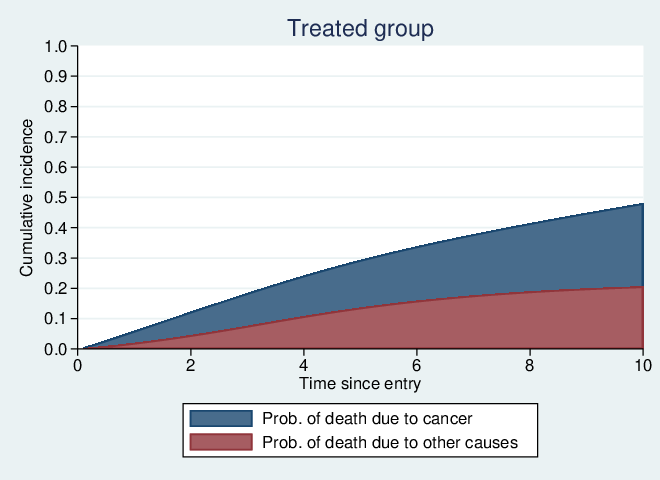
Let’s calculate the cumulative incidence functions for each cause using the predict tools. I’ll generate a time variable, and calculate the predictions for a patient in the treated group.

. range tvar 0 10 100
(1,845 missing values generated)

. predict cif1, cif outcome(1) causes(1 2) timevar(tvar) at(trt 1)
(1846 missing values generated)

. predict cif2, cif outcome(2) causes(1 2) timevar(tvar) at(trt 1)
(1846 missing values generated)

By default, causes() will include all models, but I’m being explicit here for clarity. To create a stacked plot, we need to add together the two CIFs, and then use area graphs:

. gen totalcif1 = cif1 + cif2

. twoway (area totalcif1 tvar)(area cif2 tvar), name(g1,replace)        ///
>           xtitle("Time since entry") ytitle("Cumulative incidence")   ///
>           title("Treated group") legend(cols(1)                       ///
>           order(1 "Prob. of death due to cancer"                      ///
>           2 "Prob. of death due to other causes"))                    ///
>           ylabel(,angle(h) format(%2.1f)) ylabel(0(0.1)1)             ///
>           plotregion(margin(zero))

Refer to caption — Figure 1: Stacked cumulative incidence functions

3.5 A multiple-outcome/multivariate model

Now I’ll move into the field of joint-longitudinal survival models. Joint models were first proposed by linking the submodels through the random effects only, such as:

. merlin  (stime trt M1[id]   , family(weibull, failure(died)))   ///
>         (logb time M1[id]@1 , family(gaussian))

Fitting fixed effects model:

Fitting full model:

Iteration 0:   log likelihood = -3095.8911
Iteration 1:   log likelihood =  -2494.924
Iteration 2:   log likelihood = -2367.2026
Iteration 3:   log likelihood =  -2310.837
Iteration 4:   log likelihood = -2310.5375
Iteration 5:   log likelihood = -2310.5374

Mixed effects regression model                  Number of obs     =      1,945
Log likelihood = -2310.5374
------------------------------------------------------------------------------
             |      Coef.   Std. Err.      z    P>|z|     [95% Conf. Interval]
-------------+----------------------------------------------------------------
stime:       |
         trt |   .0231889   .1749004     0.13   0.895    -.3196096    .3659873
      M1[id] |   1.233915   .1033909    11.93   0.000     1.031273    1.436557
       _cons |    -3.8462   .2687252   -14.31   0.000    -4.372892   -3.319509
  log(gamma) |   .4221851   .0711164     5.94   0.000     .2827996    .5615706
-------------+----------------------------------------------------------------
logb:        |
        time |   .0976615   .0043191    22.61   0.000     .0891962    .1061268
      M1[id] |          1          .        .       .            .           .
       _cons |    .577775   .0649576     8.89   0.000     .4504604    .7050897
  sd(resid.) |   .4912122   .0085843                      .4746722    .5083284
-------------+----------------------------------------------------------------
id:          |
      sd(M1) |   1.107264   .0470596                      1.018766     1.20345
------------------------------------------------------------------------------

By including my random intercept M1 in the complex predictor for the survival outcome, and not specifying a constraint, it will give me an association parameter, for the relationship between the subject-specific random intercept of the biomaker, and survival. Alternatively, and now more commonly, we can use the EV[] element type to link the time-dependent expected value of the biomarker, directly to the risk of event. Given we are modelling time, the timevar() must be specified in both submodels, as it will be integrated over in the survival model likelihood contribution.

. merlin  (stime trt EV[logb]             , family(weibull, failure(died))    ///
>                                                           timevar(stime))   ///
>         (logb fp(time, pow(1)) M1[id]@1 , family(gaussian) timevar(time))   ///
>         , nolog
variables created for model 2, component 1: _cmp_2_1_1 to _cmp_2_1_1

Fitting fixed effects model:

Fitting full model:

Mixed effects regression model                  Number of obs     =      1,945
Log likelihood =  -2307.676
------------------------------------------------------------------------------
             |      Coef.   Std. Err.      z    P>|z|     [95% Conf. Interval]
-------------+----------------------------------------------------------------
stime:       |
         trt |   .0218858   .1753999     0.12   0.901    -.3218916    .3656632
        EV[] |   1.279504   .1064773    12.02   0.000     1.070812    1.488196
       _cons |  -4.544086   .2929153   -15.51   0.000    -5.118189   -3.969982
  log(gamma) |   .1816336   .0725664     2.50   0.012      .039406    .3238612
-------------+----------------------------------------------------------------
logb:        |
        fp() |   .0981289   .0043134    22.75   0.000     .0896748     .106583
      M1[id] |          1          .        .       .            .           .
       _cons |   .5775447   .0649697     8.89   0.000     .4502065     .704883
  sd(resid.) |   .4912633    .008587                      .4747181    .5083852
-------------+----------------------------------------------------------------
id:          |
      sd(M1) |   1.107605   .0470632                      1.019099    1.203797
------------------------------------------------------------------------------

There’s no limit in how many and what form of association we specify, for example, we can also link the cumulative value of the biomarker (this of it as cumulative exposure), directly to survival as well.

. merlin  (stime trt EV[logb] iEV[logb]   , family(weibull, failure(died))    ///
>                                                           timevar(stime))   ///
>         (logb fp(time, pow(1)) M1[id]@1 , family(gaussian) timevar(time))   ///
>         , nolog
variables created for model 2, component 1: _cmp_2_1_1 to _cmp_2_1_1

Fitting fixed effects model:

Fitting full model:

Mixed effects regression model                  Number of obs     =      1,945
Log likelihood = -2306.8166
------------------------------------------------------------------------------
             |      Coef.   Std. Err.      z    P>|z|     [95% Conf. Interval]
-------------+----------------------------------------------------------------
stime:       |
         trt |   .0504001   .1769845     0.28   0.776    -.2964832    .3972833
        EV[] |   1.454447   .1759923     8.26   0.000     1.109508    1.799385
       iEV[] |   -.039734   .0309956    -1.28   0.200    -.1004842    .0210162
       _cons |  -4.897317   .4150173   -11.80   0.000    -5.710736   -4.083898
  log(gamma) |   .2881265   .1054815     2.73   0.006     .0813864    .4948665
-------------+----------------------------------------------------------------
logb:        |
        fp() |   .0982338   .0043145    22.77   0.000     .0897775      .10669
      M1[id] |          1          .        .       .            .           .
       _cons |    .578134   .0650171     8.89   0.000     .4507029    .7055651
  sd(resid.) |   .4912445   .0085862                      .4747009    .5083647
-------------+----------------------------------------------------------------
id:          |
      sd(M1) |   1.108471   .0471066                      1.019885    1.204753
------------------------------------------------------------------------------

Non-linearities in the association, and time-dependent effects can also be specified,

. merlin  (stime trt EV[logb] EV[logb]#fp(stime, pow(0))                            ///
>                                 , family(weibull, failure(died)) timevar(stime))  ///
>         (logb fp(time, pow(1)) M1[id]@1 , family(gaussian) timevar(time))         ///
>         , nolog
variables created for model 1, component 3: _cmp_1_3_1 to _cmp_1_3_1
variables created for model 2, component 1: _cmp_2_1_1 to _cmp_2_1_1

Fitting fixed effects model:

Fitting full model:

Mixed effects regression model                  Number of obs     =      1,945
Log likelihood = -2306.9583
------------------------------------------------------------------------------
             |      Coef.   Std. Err.      z    P>|z|     [95% Conf. Interval]
-------------+----------------------------------------------------------------
stime:       |
         trt |   .0474124    .176971     0.27   0.789    -.2994445    .3942693
        EV[] |   1.426935   .1685864     8.46   0.000     1.096512    1.757359
   EV[]#fp() |  -.1238257    .103456    -1.20   0.231    -.3265958    .0789443
       _cons |  -5.039479   .5227427    -9.64   0.000    -6.064036   -4.014922
  log(gamma) |   .3605683   .1549538     2.33   0.020     .0568644    .6642722
-------------+----------------------------------------------------------------
logb:        |
        fp() |   .0980068   .0043171    22.70   0.000     .0895455    .1064682
      M1[id] |          1          .        .       .            .           .
       _cons |   .5792938   .0650543     8.90   0.000     .4517897    .7067979
  sd(resid.) |   .4912286   .0085855                      .4746863    .5083473
-------------+----------------------------------------------------------------
id:          |
      sd(M1) |   1.108874   .0471116                      1.020277    1.205165
------------------------------------------------------------------------------

3.6 A final model

So now I’m going to bring together a lot of the previous models into one meta-merlin-model, if you will. This is purely for illustrative purposes, but hopefully gives you an idea of just how flexible merlin can be. I’m now going to generate a binary repeatedly measured variable, catpro, which is prothrombin merely categorised into above and below 12 (this is clearly an unnecessary thing to do, but purely for illustrative purposes). I will also use the artificial competing risks outcomes created above, and so bring together a joint model for two repeatedly measured outcomes, one continuous and one binary, with cause-specific competing risks survival models. Each cause-specific hazard model will have a different distribution, and we can allow for time-dependent effects/non-proportional hazards.

. gen byte catpro = prothrombin > 12

. merlin  (stime  trt                                     ///
>                 M2[id] M1[id]                           ///
>                 , family(rcs, failure(cancer) df(3))    ///
>                 timevar(stime))                         ///
>         (stime  trt trt#fp(stime, pow(0))               ///
>                 EV[logb] M1[id]                         ///
>                 , family(weibull, failure(other))       ///
>                 timevar(stime))                         ///
>         (logb   rcs(time, df(3) orthog)                 ///
>                 M1[id]@1                                ///
>                 , family(gaussian)                      ///
>                 timevar(time))                          ///
>         (catpro fp(time, powers(1))                     ///
>                 M2[id]@1                                ///
>                 , family(bernoulli)                     ///
>                 timevar(time))                          ///
>         , covariance(unstructured) nolog
variables created: _rcs1_1 to _rcs1_3
variables created for model 2, component 2: _cmp_2_2_1 to _cmp_2_2_1
variables created for model 3, component 1: _cmp_3_1_1 to _cmp_3_1_3
variables created for model 4, component 1: _cmp_4_1_1 to _cmp_4_1_1

Fitting fixed effects model:

Fitting full model:

Mixed effects regression model                  Number of obs     =      1,945
Log likelihood = -2827.9382
------------------------------------------------------------------------------
             |      Coef.   Std. Err.      z    P>|z|     [95% Conf. Interval]
-------------+----------------------------------------------------------------
stime:       |
         trt |   .0843121   .2585119     0.33   0.744    -.4223619    .5909861
      M2[id] |   .5877474   .1423448     4.13   0.000     .3087568     .866738
      M1[id] |   .6124566    .231844     2.64   0.008     .1580507    1.066863
       _cons |  -3.291482   .2618039   -12.57   0.000    -3.804608   -2.778356
-------------+----------------------------------------------------------------
stime:       |
         trt |  -.0431231   .4161423    -0.10   0.917    -.8587469    .7725008
    trt#fp() |  -.0008662   .2759082    -0.00   0.997    -.5416363    .5399039
        EV[] |   1.079582   1.306597     0.83   0.409    -1.481301    3.640466
      M1[id] |   .1642467   1.280222     0.13   0.898    -2.344943    2.673436
       _cons |  -5.311877   .8722111    -6.09   0.000     -7.02138   -3.602375
  log(gamma) |   .2798372   .2963124     0.94   0.345    -.3009244    .8605988
-------------+----------------------------------------------------------------
logb:        |
     rcs():1 |   .3046816   .0132337    23.02   0.000      .278744    .3306192
     rcs():2 |   .0678822   .0118585     5.72   0.000       .04464    .0911244
     rcs():3 |   .0136599   .0114777     1.19   0.234     -.008836    .0361558
      M1[id] |          1          .        .       .            .           .
       _cons |   .8969961   .0647674    13.85   0.000     .7700542    1.023938
  sd(resid.) |    .486531   .0085215                      .4701126    .5035228
-------------+----------------------------------------------------------------
catpro:      |
        fp() |   .5194474   .0453455    11.46   0.000     .4305718    .6083229
      M2[id] |          1          .        .       .            .           .
       _cons |  -4.618131   .3378236   -13.67   0.000    -5.280253   -3.956009
-------------+----------------------------------------------------------------
id:          |
      sd(M1) |   1.115666   .0473025                      1.026702    1.212338
      sd(M2) |   2.878879   .2668173                      2.400674     3.45234
 corr(M2,M1) |   .7836109    .034906                      .7051134    .8431351
------------------------------------------------------------------------------

There’s four outcome models, and two random effects, so it takes some time, but we get there in about 16 minutes on my laptop. It’s trivial to extend this model, for example adding random slopes, or different ways of linking the submodels, or incorporating non-linear effects, be they for continuous covariates or time.

4 Discussion

I have given a broad overview of merlin’s capabilities, and potential, in the field of data analysis. I’ve described the fundamental syntax, and through worked examples, illustrated some of the areas of statistical modelling that can be applied using merlin. I’ll finish with some final thoughts.

4.1 The curse of generality

When implementing a software package that can do many things, one of the challenging tasks is to balance said generality, with computational speed. merlin is not the quickest. It’s current implementation is a gf0 evaluator, which means it uses Stata’s internal finite difference routines within the ml engine to calculate the score and Hessian, which means a lot of calls to the evaluator program. Furthermore, merlin has to cover a lot of different settings and options, which inevitably mean a lot of storing information within its main object. Now a lot of that is alleviated through use of pointers and other clever things, but it will still result in some overheads. You will get speed gains if you implement a specific command, from scratch, designed for a specific setting.

4.2 Shell commands

Firstly, the syntax of merlin is not the simplest. This is of course because it has to accommodate a lot of different options and techniques. This opens up more room to go wrong. Secondly, it is rather challenging to obtain good starting values for a command that can fit anything, and good starting values can be crucial to improve convergence.

This motivates the writing of shell commands, i.e. ado files specifically written to handle specific classes of merlin models. This allows a much simpler and cleaner syntax, and the ability to hard code initial value fitting routines. Under the hood, and unbeknownst to most users, the shell command will call merlin. I’m working on a few of these.

4.3 Concluding remarks

There is a multitude of future directions to take merlin in. Some of which include; adding analytic derivatives for computational speed gains, extending the allowed random effects distributions to allow things like mixtures of Gaussians, and providing more tools for postestimation, including dynamic prediction capabilities.

The latest stable version of merlin can be installed by typing ssc install merlin in Stata. The development version can be installed using:

net install merlin, from(https://www.mjcrowther.co.uk/code/merlin)

I hope you find merlin useful.

About the author

Michael J. Crowther is a Lecturer in Biostatistics at the University of Leicester. He works heavily in methods and software development, particularly in the field of survival analysis. He is currently part funded by a MRC New Investigator Research Grant (MR/P015433/1).

References

Crowther (2017) Crowther, M. J. 2017. Extended multivariate generalised linear and non-linear mixed effects models. arXiv preprint arXiv:1710.02223 .
Crowther et al. (2013) Crowther, M. J., K. R. Abrams, and P. C. Lambert. 2013. Joint modeling of longitudinal and survival data. Stata J 13(1): 165–184.
Crowther and Lambert (2013) Crowther, M. J., and P. C. Lambert. 2013. stgenreg: A Stata package for the general parametric analysis of survival data. J Stat Softw 53(12).
Crowther and Lambert (2014) . 2014. A general framework for parametric survival analysis. Stat Med 33(30): 5280–5297. URL http://dx.doi.org/10.1002/sim.6300.
Crowther et al. (2014) Crowther, M. J., M. P. Look, and R. D. Riley. 2014. Multilevel mixed effects parametric survival models using adaptive Gauss-Hermite quadrature with application to recurrent events and individual participant data meta-analysis. Stat Med 33(22): 3844–3858. URL http://dx.doi.org/10.1002/sim.6191.
Murtaugh et al. (1994) Murtaugh, P., E. Dickson, M. Van Dam, G. Malincho, and P. Grambsch. 1994. Primary biliary cirrhosis: Prediction of short-term survival based on repeated patient visits. Hepatology 20: 126–134.
Rabe-Hesketh et al. (2002) Rabe-Hesketh, S., A. Skrondal, and A. Pickles. 2002. Reliable estimation of generalized linear mixed models using adaptive quadrature. Stata J 2: 1–21.
Rabe-Hesketh et al. (2005) . 2005. Maximum likelihood estimation of limited and discrete dependent variable models with nested random effects. Journal of Econometrics 128(2): 301–323.