Analytic evaluation of Hecke eigenvalues for classical modular forms

We thank the Fulbright Commission of Ecuador for making the collaboration of Armendáriz, Terán and Ryan possible. We also thank David Farmer for some helpful conversations.

We have a quantity defined as

The numerator and denominator can be approximated to $x_{A}$, resp. $y_{A}$. In particular, we think of $x_{A}$ as a numerical approximation to $T_{p}(f)(z_{0})$, for some $z_{0}\in\mathbb{H}$, and $y_{A}$ as $f(z_{0})$.

Given $\varepsilon>0$, we seek values of $\varepsilon_{x}$ and $\varepsilon_{y}$ ensure that

The value of the parameter $h$ can be chosen in such a way that the calculations of $x_{A}$ and of $y_{A}$ are roughly of the same level of difficulty.

In addition to the error in a quotient, we also point out that we need to take into account error in a sum. In particular, to compute $T_{p}(f)(z_{0})$ for some $z_{0}\in\mathbb{H}$ we need to evaluate $f$ at $p+1$ (respectively, $p$) if $p$ does not divide (respectively, does divide) the level $N$. In particular, suppose $x=\sum_{i=1}^{N}x^{(i)}$, $x_{A}=\sum_{i=1}^{N}x_{A}^{(i)}$ and that $|x^{(i)}-x^{(i)}_{A}|<\varepsilon_{i}$. We want an $\varepsilon_{i}$ so that $|x^{(i)}-x^{(i)}_{A}|<\varepsilon_{i}$ guarantees $|x-x_{A}|<\varepsilon$. By the triangle inequality, we can let $\varepsilon_{i}=\tfrac{\varepsilon}{N}$.

Let $f\in S_{k}^{\text{new}}(\Gamma_{0}(N))$ be a classical newform of weight $k$ with Fourier expansion

Given $T\in\mathbb{N}$, we consider the truncated expansion

Let

The conditions on $T$ make it clear that larger values of $y$ allow for shorter truncations.

When our modular form is of level 1, we can use the modularity of $f$ to move the evaluation from the point $z=x+iy$ to another point $(az+b)/(cz+d)$ that has a larger imaginary part:

The group $\textrm{SL}_{2}(\mathbb{Z})$ is generated by the matrices

The former does not change the imaginary part, so it is enough to consider the latter:

This leads us to a very simple approach: given $z=x+iy$, first use the periodicity of $f$ to ensure $|x|\leq 1/2$. If $x^{2}+y^{2}\geq 1$, then evaluate $f$ at $z$; otherwise evaluate $f$ at $-1/z$ and use

In Section 3 we stated and proved some error bounds. Recall the notation of Proposition 6. In particular, we approximate $\lambda_{p}$ ($z_{A}$ in the notation of the Proposition) by taking the quotient $\tfrac{T_{p}(f)(z_{0})}{z_{0}}$ (denoted $\tfrac{x_{A}}{y_{A}}$ in the Proposition). We want to compute $\lambda_{p}$ to a chosen number of digits of accuracy.

In order to use the results of Proposition 6 in practice, we need a lower bound on $|y_{A}|$ and an upper bound on $|z_{A}|$ (which can be obtained from the lower bound on $|y_{A}|$ and an upper bound on $|x_{A}|$).

How do we bound $|x_{A}|$? We compute a very coarse estimate $\tilde{x}$ to $x$, with $\tilde{\varepsilon}_{x}$ just small enough that $|\tilde{x}|-2\tilde{\varepsilon}_{x}>0$. (We can start with $\tilde{\varepsilon}_{x}=0.1$ and keep dividing by $10$ until the condition holds.) Later we will make sure that $\varepsilon_{x}$ is smaller than $\tilde{\varepsilon}_{x}$.

Then we know that

so

giving us lower and upper bounds on $|x_{A}|$. A similar argument works for $|y_{A}|$.

Our code finds the $T$ described in Proposition 7 as follows. We increment $T$ by 1 until both conditions of Proposition 7 are met.

The user is free to choose any value of $z_{0}$ at which to evaluate the modular form; when $z_{0}$ is chosen to have a moderately large imaginary part, then $T=1$ satisfies both conditions. This is problematic because then the difference $|f(z)-f_{T}(z)|$ becomes zero and we are not really approximating anything. In this case, we arbitrarily increase $T$ to 100.

Our code allows for the user to choose any value of $z_{0}$ at which to evaluate the modular form $f$. When $z_{0}$ is closer to the real axis, our algorithm slows down considerably. For such $z_{0}$ we need to compute a very large number of Fourier coefficients since in Proposition 7 the value of $T$ becomes quite large.

As described in Remark 8, we use inversion across the unit circle or the circle centered at the origin and of radius $1/\sqrt{N}$ to make the imaginary part bigger.

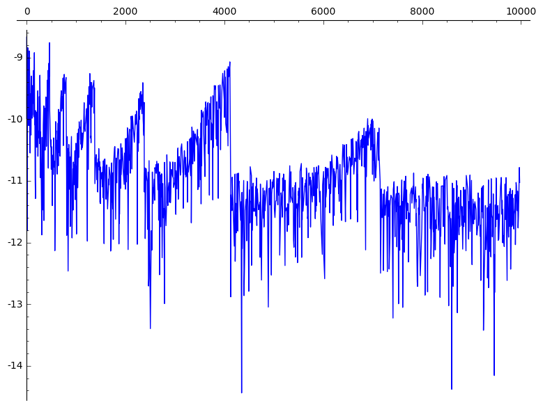
In this section, we compare the modular symbol method as implemented in Sage [10] to our method. In Figure 2 we see the results of the following computation: for each $p$ we compute the $p$th Hecke eigenvalue in both ways (using modular symbols and using our analytic approach) and take $\log_{10}$ of the absolute value of the difference. We see in Figure 2 that for a fixed $F\in S_{24}(1)$ the two methods agree to at least $10^{-8}$. In this section we use $\lambda_{p}$ to denote the $p$th Hecke eigenvalue computed via modular symbols and $\tilde{\lambda}_{p}$ to denote the $p$th Hecke eigenvalue approximated using our analytic approach.

In Table 1 we highlight some timings in which we computed Hecke eigenvalues using both methods. The results of our method are computed via code like

sage: F12 = Newforms(1, 12, names=’a’)[0]
sage: p = next_prime(10000)
sage: err = 0.1
sage: e = eigenvalue_numerical(F12, p, err)
sage: e
-5.758585642481476962744000?e21

and the results of the modular symbols method are computed via code like¹¹ 1 We have chosen this somewhat cryptic way of computing the eigenvalue via modular symbols over more obvious and readable ones for two reasons: (a) Sage uses aggressive caching of various intermediate results, which makes it hard to obtain useful timings from repeated evaluations of the same eigenvalue; (b) it is the quickest way of getting the eigenvalue, since the more user-facing methods perform other bookkeeping that is not absolutely necessary for our purpose and can easily take up the bulk of the running time. For instance, e = F12[p] for the example given in the text takes a little over 9 minutes, compared to about 1 second for the more verbose modular symbols method.

sage: F12 = Newforms(1, 12, names=’a’)[0]
sage: p = next_prime(10000)
sage: ms = F12.modular_symbols(1)
sage: T = ms._eigen_nonzero_element(p)
sage: e = ms._element_eigenvalue(T, name=’b’)
sage: e
-5758585642481476962744

A clear difference between the two methods is the number of Fourier coefficients required for the computation of the $p$th Hecke eigenvalue. In Figure 3 we see how few coefficients are needed to compute $\tilde{\lambda}_{p}$.

In the previous sections we described how to evaluate $f$ using its Fourier expansions and in Table 1 we provide some timings using this method. In this section we focus on the specific case of level 1 and describe a faster way to evaluate $f$. It is well known that the ring of modular forms of level 1 is generated by the Eisenstein series of levels 4 and 6. What we do in this case is the following: Let $z\in\mathbb{H}$:

1. 1.

   calculate roughly $k/12$ coefficients of the modular form $f$, $E_{4}$ and $E_{6}$;

2. 2.

   identify a basis for $S_{k}(1)$ by finding $T=\{(a,b)\in\mathbb{Z}:4a+6b=k-12\}$ and computing the first $k/12$ coefficients of $\Delta\cdot E_{4}^{a}E_{6}^{b}$ for all $(a,b)\in T$;

3. 3.

   express $f$ as a linear combination of the basis elements found in Step 2 and replace $\Delta$ with $\tfrac{E_{6}^{2}-E_{4}^{3}}{1728}$;

4. 4.

   calculate $x=E_{4}(z)$, $y=E_{6}(z)$ and the evaluate $f(z)$ by taking the appropriate algebraic combination of $x$ and $y$.

Numerical experiments suggest that this approach via evaluation of Eisenstein series is particularly beneficial in the case of large weights (see Table 1).

References

- [1] D. Armendáriz, O. Colman, N. Coloma, A. Ghitza, N. C. Ryan, and D. Terán. SageMath code for the analytic calculation of the Hecke eigenvalues of classical modular forms. https://github.com/nathancryan/analytic-evaluation-classical-modular-forms, 2019. [Online; accessed 29-Sep-2019].
- [2] K. Belabas and H. Cohen. Modular forms in Pari/GP. Res. Math. Sci., 5(3):Paper No. 37, 19, 2018.
- [3] A. R. Booker, A. Strömbergsson, and A. Venkatesh. Effective computation of Maass cusp forms. Int. Math. Res. Not., 2006. Art. ID 71281, 34 pp.
- [4] W. Bosma, J. Cannon, and C. Playoust. The Magma algebra system. I. The user language. J. Symbolic Comput., 24(3-4):235–265, 1997. Computational algebra and number theory (London, 1993).
- [5] B. Edixhoven and J-M. Couveignes, editors. Computational aspects of modular forms and Galois representations, volume 176 of Annals of Mathematics Studies. Princeton University Press, Princeton, NJ, 2011.
- [6] D. A. Hejhal. On eigenfunctions of the Laplacian for Hecke triangle groups. In Emerging applications of number theory, pages 291–315. Springer, 1999.
- [7] F. Johansson. Arb: efficient arbitrary-precision midpoint-radius interval arithmetic. IEEE Transactions on Computers, 66:1281–1292, 2017.
- [8] D. H. Lehmer. The vanishing of Ramanujan’s function . Duke Math. J, 14:429–433, 1947.
- [9] W. A. Stein and P. E. Gunnells. Modular forms, a computational approach, volume 79. American Mathematical Society Providence, RI, 2007.
- [10] W. A. Stein et al. Sage Mathematics Software (Version 8.8). The Sage Development Team, 2019. http://www.sagemath.org.
- [11] The PARI Group, Univ. Bordeaux. PARI/GP version 2.11.2, 2019. Available from http://pari.math.u-bordeaux.fr/.
- [12] C. Wuthrich. Numerical modular symbols for elliptic curves. Math. Comp., 87(313):2393–2423, 2018.