Quantum gyro-electric effect: Photon spin-1 quantization in continuum topological bosonic phases

In two spatial dimensions (and one temporal dimension), the propagation of charge is restricted to the $x$-$y$ plane. This limits the degrees of freedom of both the electromagnetic field and the induced response of a material (Fig. 3). Therefore, we focus on strictly transverse-magnetic (TM) waves, meaning there are only 3 unique components of the field. From first principles (Appendix A), we derive the corresponding wave equation of the 2D photon coupled to matter,

$$\mathcal{H}_{0}(\mathbf{k})f=\omega\mathcal{M}(\omega,\mathbf{k})f,\qquad f=\begin{bmatrix}E_{x}\\ E_{y}\\ H_{z}\end{bmatrix},$$

(2)

where $f$ is the TM polarization state (wavefunction) of the electromagnetic field. In the absence of matter, $\mathcal{H}_{0}(\mathbf{k})$ are the vacuum Maxwell equations in momentum space,

$$\mathcal{H}_{0}(\mathbf{k})=k_{x}\hat{S}_{x}+k_{y}\hat{S}_{y}=\begin{bmatrix}0&0&-k_{y}\\ 0&0&k_{x}\\ -k_{y}&k_{x}&0\\ \end{bmatrix}.$$

(3)

Notice that $\mathcal{H}_{0}(\mathbf{k})=\mathbf{k}\cdot\mathbf{S}$ represents optical helicity, i.e. the projection of momentum $\mathbf{k}$ onto the spin $\mathbf{S}$. We identify these spin-1 operators $\hat{S}_{x}$ and $\hat{S}_{y}$ that satisfy the angular momentum algebra $[\hat{S}_{x},\hat{S}_{y}]=i\hat{S}_{z}$,

$$\hat{S}_{x}=\begin{bmatrix}0&0&0\\ 0&0&1\\ 0&1&0\end{bmatrix},~~\hat{S}_{y}=\begin{bmatrix}0&0&-1\\ 0&0&0\\ -1&0&0\end{bmatrix},~~\hat{S}_{z}=\begin{bmatrix}0&-i&0\\ i&0&0\\ 0&0&0\end{bmatrix}.$$

(4)

Here, $(\hat{S}_{z})_{ij}=-i\epsilon_{ijz}$ is the generator of rotations in the $x$-$y$ plane and is represented by the antisymmetric matrix. $\hat{S}_{z}$ will be foundational when discussing spin-1 symmetries in 2D.

The linear response function of the 2D material $\mathcal{M}$ is dependent on continuous variables $\omega$ and $\mathbf{k}$,

$$\mathcal{M}(\omega,\mathbf{k})=\begin{bmatrix}\varepsilon_{xx}&\varepsilon_{xy}&\chi_{x}\\ \varepsilon_{xy}^{*}&\varepsilon_{yy}&\chi_{y}\\ \chi_{x}^{*}&\chi_{y}^{*}&\mu\end{bmatrix},~~\begin{array}[]{ll}D_{i}=\varepsilon_{ij}E^{j}+\chi_{i}H_{z},\\ \\ B_{z}=\chi_{i}^{*}E^{i}+\mu H_{z},\\ \end{array}$$

(5)

which compactly represents the constitutive relations. We include all possible material responses as a generalization - for instance magneto-electricity $\chi_{i}$ and birefringence in $\varepsilon_{ij}$. However, based on symmetry constraints, we will show that only certain parameters of $\mathcal{M}$ are important in the topological classification.

Alas, Eq. (2) poses a problem; it does not represent a proper first-order in time Hamiltonian since the response function $\mathcal{M}(\omega,\mathbf{k})$ is dependent on its own eigenvalue. Nevertheless, we can prove that it is derived from a first-order Hamiltonian by exploiting stringent symmetry properties. We demand Hermiticity $\mathcal{M}=\mathcal{M}^{\dagger}$ such that the response is lossless. We also require positive definiteness $\bar{\mathcal{M}}=\partial_{\omega}(\omega\mathcal{M})>0$ to ensure the energy density is non-negative and admits proper normalization $f^{\dagger}\bar{\mathcal{M}}f>0$. The response must be causal (Kramers-Kronig) and obey the reality condition $\mathcal{M}(\omega,\mathbf{k})=\mathcal{M}^{*}(-\omega,-\mathbf{k})$, guaranteeing the electromagnetic fields are real-valued [45]. Two additional constraints should also be considered for realistic materials. Stability at static equilibrium $\mathcal{M}(0,\mathbf{k})=\bar{\mathcal{M}}(0,\mathbf{k})>0$, and the ultraviolet limit $\lim_{\omega\to\infty}\mathcal{M}(\omega,\mathbf{k})=\mathds{1}_{3}$. Here, $\mathds{1}_{3}$ is the $3\times 3$ identity matrix and the limit implies transparency at high-frequency $\omega\to\infty$, as the material cannot respond to sufficiently fast temporal oscillations.

Combining all the above criteria, we find that the response function can always be decomposed as a discrete summation of oscillators [27, 30, 46],

$$\mathcal{M}(\omega,\mathbf{k})=\mathds{1}_{3}-\sum_{\alpha}\frac{\mathcal{C}^{\dagger}_{\alpha\mathbf{k}}\mathcal{C}_{\alpha\mathbf{k}}}{\omega_{\alpha\mathbf{k}}(\omega-\omega_{\alpha\mathbf{k}})}.$$

(6)

$\alpha$ labels any arbitrary bosonic excitation in the material, such as an exciton or phonon, which couples linearly to the electromagnetic fields via the $3\times 3$ tensor $\mathcal{C}_{\alpha\mathbf{k}}$. $\omega_{\alpha\mathbf{k}}$ is the resonant energy of the oscillator and corresponds to a first-order pole of the response function. Note both $\mathcal{C}_{\alpha\mathbf{k}}$ and $\omega_{\alpha\mathbf{k}}$ are in general $\mathbf{k}$ dependent. We emphasize that the response function is consistent with previous work on gyrotropic plasmas [47, 48]. However, our key advance is that the tensors $\mathcal{C}_{\alpha\mathbf{k}}$, characterizing the collective light-matter excitations, carry information of spin and orbital angular momentum.

A detailed derivation of the continuum electromagnetic Hamiltonian $H(\mathbf{k})$ is presented in Appendix B. To accomplish this, we expand the response function $\mathcal{M}(\omega,\mathbf{k})$ in terms of 3-component matter oscillators $\psi_{\alpha}$. These represent internal polarization and magnetization modes of the material,

$$\psi_{\alpha}=\frac{\mathcal{C}_{\alpha\mathbf{k}}f}{\omega-\omega_{\alpha\mathbf{k}}},\qquad\omega\psi_{\alpha}=\omega_{\alpha\mathbf{k}}\psi_{\alpha}+\mathcal{C}_{\alpha\mathbf{k}}f.$$

(7)

We now define $u$ as the generalized state vector of the electromagnetic problem, accounting for the photon $f$ and all possible internal excitations $\psi_{\alpha}$,

$$H(\mathbf{k})u=\omega u,\qquad u=\begin{bmatrix}f&\psi_{1}&\psi_{2}&\ldots\end{bmatrix}^{\intercal},$$

(8)

which satisfies a first-order Hamiltonian wave equation. Notice that contraction of $u$ naturally reproduces the energy density upon summation over all degrees of freedom $u^{\dagger}u=f^{\dagger}\bar{\mathcal{M}}f$, with $\bar{\mathcal{M}}=\partial_{\omega}(\omega\mathcal{M})>0$ always positive definite. The continuum Hamiltonian $H(\mathbf{k})$ acting on $u$ is given concisely as,

$$H(\mathbf{k})=\begin{bmatrix}\mathcal{H}_{0}(\mathbf{k})+\sum_{\alpha}\omega_{\alpha\mathbf{k}}^{-1}\mathcal{C}^{\dagger}_{\alpha\mathbf{k}}\mathcal{C}_{\alpha\mathbf{k}}&~~\mathcal{C}^{\dagger}_{1\mathbf{k}}~~&~~\mathcal{C}^{\dagger}_{2\mathbf{k}}~~&\ldots\\ \mathcal{C}_{1\mathbf{k}}&\omega_{1\mathbf{k}}&0&\ldots\\ \mathcal{C}_{2\mathbf{k}}&0&\omega_{2\mathbf{k}}&\ldots\\ \vdots&\vdots&\vdots&\ddots\end{bmatrix}.$$

(9)

This eigenvalue problem generates the complete spectrum of quasiparticle eigenstates,

$$H_{\mathbf{k}}u_{n\mathbf{k}}=\omega_{n\mathbf{k}}u_{n\mathbf{k}},$$

(10)

and the eigenstates are normalized to the energy density $u^{\dagger}_{n\mathbf{k}}u_{n\mathbf{k}}=f^{\dagger}_{n\mathbf{k}}\bar{\mathcal{M}}(\omega_{n\mathbf{k}},\mathbf{k})f_{n\mathbf{k}}=1$. Moreover, the eigenenergies $\omega_{n\mathbf{k}}$ are the $n$ non-trivial roots of the characteristic equation,

$$\det[\mathcal{H}_{0}(\mathbf{k})-\omega\mathcal{M}(\omega,\mathbf{k})]=0,\qquad\omega=\omega_{n}(\mathbf{k}),$$

(11)

proving that the response function $\mathcal{M}(\omega,\mathbf{k})$ is derived from a first-order Hamiltonian $H(\mathbf{k})$.

Our goal is to develop a continuum topological theory that accounts for both spatiotemporal dispersion and the inherent bosonic properties of light. Due to the unbounded nature of the momentum space $\mathbb{R}^{2}$, continuum Chern numbers are usually ill-defined. Nevertheless, as long as the system is properly regularized, continuum field theories are possible and can be incredibly powerful tools to study long wavelength topological physics [49, 50, 51]. A necessary condition is one-point compactification of the momentum space [52, 53, 54], which governs the high-$k$ asymptotic behavior of the Hamiltonian. This requirement is well understood in condensed matter and demands the Hamiltonian approach a directionally independent value,

$$\lim_{k\to\infty}H(\mathbf{k})\to H(k),$$

(12)

where $k=\sqrt{\mathbf{k}\cdot\mathbf{k}}$ is the magnitude of the wavevector. In this way, all limits at infinity are mapped into the same point and satisfy a “periodic” boundary condition. The momentum space is closed and topologically equivalent to the Reimann sphere $\mathbb{R}^{2}\simeq S^{2}$ (Fig. 3). Hence, Chern numbers are quantized. A rigorous proof is presented in Appendix C.

This constraint has important implications in continuum photonic media. Since Maxwell’s equations are strictly first-order in spatial derivatives (Eq. (3)), one-point compactification can only be satisfied by introducing non-locality [55, 56]. Non-locality (or spatial dispersion) is the momentum dependence of linear response - commonly ignored in photonics problems, DC transport measurements, as well as Faraday rotation experiments. However, we strongly emphasize that the high-$k$ behavior cannot be neglected even in the long wavelength continuum theory. These deep sub-wavelength components encode global information of the fields and are essential to properly describe the topological physics. By exploiting rotational symmetry, we will show that the asymptotic behavior of the Hamiltonian $H(\mathbf{k})$ and by extension, the response function $\mathcal{M}(\omega,\mathbf{k})$, is naturally regularized and predicts new bosonic phases of matter.

If the two dimensional crystal has a center (at least 3-fold cyclic [57, 58]), the continuum Hamiltonian is rotationally symmetric about $z$,

$$\mathcal{R}^{-1}H(\mathcal{R}\mathbf{k})\mathcal{R}=H(\mathbf{k}),\qquad\mathcal{R}(2\pi)=\mathds{1}_{3},$$

(13)

and the eigenenergies $\omega=\omega_{n}(k)$ depend only on the magnitude of $k$. Note that $\mathcal{R}$ is diagonal in $u$, meaning the photon and each oscillator is rotated individually, $f\to\mathcal{R}f$ and $\psi_{\alpha}\to\mathcal{R}\psi_{\alpha}$. In this case $\mathcal{R}(\theta)$ is a continuous rotation,

$$\mathcal{R}(\theta)=\exp[i\theta\hat{S}_{z}]=\begin{bmatrix}\cos\theta&\sin\theta&0\\ -\sin\theta&\cos\theta&0\\ 0&0&1\end{bmatrix},$$

(14)

and can be expressed as the exponential of the spin-1 generator $(\hat{S}_{z})_{ij}=-i\epsilon_{ijz}$. This represents an element of SO(3) in the subspace of $\mathbb{R}^{2}$ [59], as all rotations occur in the $x$-$y$ plane. We stress that the vector representation is bosonic, meaning the quasiparticles return in phase under cyclic revolution $\mathcal{R}(2\pi)=\mathds{1}_{3}$.

Since the Hamiltonian possesses a continuous rotational symmetry, the total angular momentum (TAM) is conserved,

$$[\hat{J}_{z},H(\mathbf{k})]=0,\qquad\hat{J}_{z}=\hat{L}_{z}+\hat{S}_{z}.$$

(15)

Eq. (13) and (15) are equivalent statements in this context. Here, $\hat{L}_{z}$ is the orbital angular momentum (OAM) operator in 2D $\mathbf{k}$-space and can be expressed in polar coordinates as,

$$\hat{L}_{z}=-ik_{x}\frac{\partial}{\partial k_{y}}+ik_{y}\frac{\partial}{\partial k_{x}}=-i\partial_{\phi}.$$

(16)

Eigenstates of the OAM are well known and represent quantized azimuthal charges,

$$\hat{L}_{z}|l\rangle=l|l\rangle,\qquad|l\rangle=\exp(il\phi),$$

(17)

where $l\in\mathbb{Z}$ is any integer.

Conversely, eigenstates of the spin angular momentum (SAM) represent states of quantized polarization, transverse to the $x$-$y$ plane,

$$\hat{S}_{z}\mathbf{e}=m\mathbf{e}.$$

(18)

The matrix form of $\hat{S}_{z}$ is given in Eq. (4). For photons, the spin is an integer $m=\pm 1,0$ and takes one of three discrete values. First, we have the $m=\pm 1$ spin states,

$$\mathbf{e}_{\pm}=\frac{1}{\sqrt{2}}\begin{bmatrix}1\\ \pm i\\ 0\end{bmatrix},\qquad\hat{S}_{z}\mathbf{e}_{\pm}=\pm\mathbf{e}_{\pm}.$$

(19)

$\mathbf{e}_{\pm}$ are resonant electric ($H_{z}=0$) counter-rotating states. Secondly, we have the $m=0$ spin state, which is resonant magnetic ($E_{i}=0$) and irrotational,

$$\mathbf{e}_{0}=\begin{bmatrix}0\\ 0\\ 1\end{bmatrix},\qquad\hat{S}_{z}\mathbf{e}_{0}=0.$$

(20)

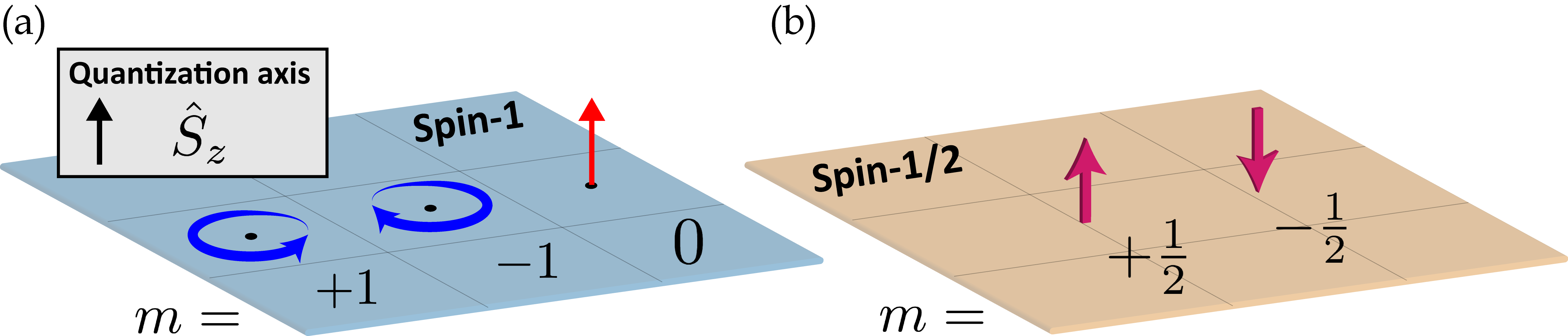
A visualization of the quantized spin-1 states is displayed in Fig. 1(a) and this is compared to quantized spin-½ states in Fig. 1(b). In Sec. IV, we will prove that these spin quantized eigenstates naturally arise at high-symmetry $\mathbf{k}$ points in 2+1D bosonic phases.

At an arbitrary momentum $\mathbf{k}$, the quasiparticles $u_{n\mathbf{k}}$ are not eigenstates of $\hat{L}_{z}$ or $\hat{S}_{z}$. Instead, they are eigenstates of the total angular momentum $\hat{J}_{z}=\hat{L}_{z}+\hat{S}_{z}$,

$$\hat{J}_{z}u_{n\mathbf{k}}=j_{n}u_{n\mathbf{k}},\qquad j_{n}\in\mathbb{Z},$$

(21)

where $j_{n}$ is an integer for bosons. Since $\hat{J}_{z}$ is a differential operator, the choice of $j_{n}$ represents a particular Berry gauge for the eigenstates. This gauge is single-valued for all $\mathbf{k}$ with the possible exception of two points, $k_{p}=0$ and $k_{p}=\infty$. These are called high-symmetry points (HSPs). At these specific momenta, the Hamiltonian is rotationally invariant [60],

$$\mathcal{R}^{-1}H(k_{p})\mathcal{R}=H(k_{p}),\qquad[\hat{S}_{z},H(k_{p})]=0,$$

(22)

which follows immediately from Eq. (13) and (15). In the continuum theory, $k_{p}=0$ is a HSP because the origin always rotates into itself. Owing to one-point compactification (Eq. (12)), $k_{p}=\infty$ is also a HSP. This is clear by direct inspection of the Riemann sphere in Fig. 3. A rotation in the plane of $\mathbb{R}^{2}$ rotates $S^{2}$ about its axis, keeping both $k_{p}=0$ and $k_{p}=\infty$ fixed. Invariance at $k_{p}=\infty$ is therefore imperative to describe continuum topological theories.

At HSPs the SAM of any eigenstate $u_{n\mathbf{k}}$ is quantized and this is guaranteed by symmetry (Eq. (22)). Still, the Berry gauge may be multi-valued here due to the OAM - known as a phase singularity [61],

$$\lim_{k\to k_{p}}u_{n}(\mathbf{k})\to u_{n}(k_{p})\exp\left[il_{n}(k_{p})\phi\right],$$

(23)

$$\hat{S}_{z}u_{n}(k_{p})=m_{n}(k_{p})u_{n}(k_{p}),$$

(24)

where $j_{n}=l_{n}(k_{p})+m_{n}(k_{p})$ at HSPs. We come to an important revelation from Eq. (23). If the spin does not change within the eigenstate dispersion $m_{n}(0)=m_{n}(\infty)$, we can remove the phase singularity at both points simultaneously $l_{n}(0)=l_{n}(\infty)=0$, such that the Berry gauge $j_{n}=m_{n}(0)=m_{n}(\infty)$ is single-valued for all $\mathbf{k}$.

However, if the spin changes within the dispersion $m_{n}(0)\neq m_{n}(\infty)$, this procedure is impossible. The Berry gauge is always multi-valued because the singularity $l_{n}(k_{p})\neq 0$ cannot be resolved at $k_{p}=0$ and $k_{p}=\infty$ simultaneously. This is a non-trivial topology. The physical interpretation is simple but profound; since the TAM is conserved for each eigenstate $\Delta j_{n}=0$, the OAM $\Delta l_{n}=l_{n}(\infty)-l_{n}(0)\neq 0$ must change to compensate for the SAM,

$$\Delta l_{n}=-\Delta m_{n}=m_{n}(0)-m_{n}(\infty).$$

(25)

We will now prove that Eq. (25) fundamentally defines the Chern classification of 2+1D bosonic phases.

Utilizing the eigenstates of the Hamiltonian in Eq. (10); we obtain the Berry connection by varying a quasiparticle with respect to the momentum,

$$\mathbf{A}_{n}(\mathbf{k})=-iu_{n\mathbf{k}}^{\dagger}\partial_{\mathbf{k}}u_{n\mathbf{k}}.$$

(26)

Applying the curl produces the gauge invariant Berry curvature $F_{n}(\mathbf{k})=\hat{\mathbf{z}}\cdot[\partial_{\mathbf{k}}\times\mathbf{A}_{n}(\mathbf{k})]$. The Chern number $C_{n}$ is a global topological invariant and is traditionally found by integrating $F_{n}$ over the 2D Brillouin zone - i.e. the torus $\mathbb{T}^{2}=S^{1}\times S^{1}$. For continuum theories, we integrate over the entire 2D momentum space $\mathbb{R}^{2}$,

$$C_{n}=\frac{1}{2\pi}\iint_{\mathbb{R}^{2}}F_{n}(\mathbf{k})~d^{2}\mathbf{k}.$$

(27)

When properly regularized, the planar manifold is topologically equivalent to the Riemann sphere $\mathbb{R}^{2}\simeq S^{2}$ and the Chern number is quantized (Appendix C).

Although photonic Chern numbers have been defined, neither the high-$k$ behavior nor the inherent bosonic properties have been addressed. With this in mind, we return to the Berry connection $\mathbf{A}_{n}$ in polar coordinates $\partial_{\mathbf{k}}=\hat{\mathbf{k}}\partial_{k}+\hat{\boldsymbol{\phi}}\partial_{\phi}$,

$$\mathbf{A}_{n}(\mathbf{k})=\hat{\mathbf{k}}A_{n}^{k}(k)+\hat{\boldsymbol{\phi}}A_{n}^{\phi}(k).$$

(28)

Due to rotational symmetry, the polar components of $\mathbf{A}_{n}$ depend only on $k$. Furthermore, we can connect the Berry potential $A_{n}^{\phi}$ directly to the OAM,

$$A_{n}^{\phi}(k)=-iu_{n\mathbf{k}}^{\dagger}\partial_{\phi}u_{n\mathbf{k}}=\langle\hat{L}_{z}\rangle_{n}.$$

(29)

Here, $\langle\hat{L}_{z}\rangle_{n}$ is the expectation value of the OAM for the $n^{\textrm{th}}$ eigenstate. This corresponds to a Berry curvature $F_{n}$ of,

$$F_{n}(k)=\partial_{k}\langle\hat{L}_{z}\rangle_{n}.$$

(30)

When integrating over all momenta $d^{2}\mathbf{k}=dkd\phi$, we find that the continuum Chern number $C_{n}$ is determined solely by the phase singularities at HSPs,

$$C_{n}=\int_{0}^{\infty}dk~\partial_{k}\langle\hat{L}_{z}\rangle_{n}=\langle\hat{L}_{z}\rangle_{n}|_{0}^{\infty}=\Delta l_{n},$$

(31)

precisely the change in OAM. Substituting for $\Delta l_{n}=-\Delta m_{n}$ in Eq. (25), we attain an elegant expression for the Chern number,

$$C_{n}=\Delta l_{n}=m_{n}(0)-m_{n}(\infty).$$

(32)

Eq. (32) is one of the central results of this paper and is valid for both fermionic and bosonic representations. Essential differences between the two are immediately apparent.

For a spin-½ electron, quanta take one of two half-integer values $m_{n}=\pm\frac{1}{2}$. Consequently, we find only one truly distinct fermionic phase,

$$\textrm{fermion}:\qquad C_{n}=\pm 1,0.$$

(33)

However, for the spin-1 photon, quanta take three integer values $m_{n}=\pm 1,0$. We discover two unique bosonic phases,

$$\textrm{boson}:\qquad C_{n}=\pm 2,\pm 1,0.$$

(34)

One with even parity $C_{n}=\pm 2$ and one with odd $C_{n}=\pm 1$. Even parity corresponds to a change from $m_{n}(0)=\pm 1$ to $m_{n}(\infty)=\mp 1$ at HSPs. This phase is familiar in interacting bosonic systems and is identified with a single gapless boson at the edge [8, 10, 9, 11, 12, 13] - not two as we might expect from fermionic Chern number arguments. Odd parity bosonic phases are quite exotic in this regard [62, 63]. This phase corresponds to a change from $m_{n}(0)=\{0,\pm 1\}$ to $m_{n}(\infty)=\{\pm 1,0\}$ at HSPs.

We now derive the asymptotic behavior of the Hamiltonian $H(\mathbf{k})$ to ensure the continuum theory is properly regularized at $k\to\infty$. This will help us discover the precise form of the response function $\mathcal{M}(\omega,\mathbf{k})$ and the order of non-locality necessary to describe a topological field theory. Non-locality plays two equally important roles in this context - it distinguishes between trivial and non-trivial phases. If high-$k$ components are ignored, it is impossible to define either of these phases in the continuum.

From Eq. (6) and (9), rotational symmetry implies the coupling tensors obey $\mathcal{R}^{-1}\mathcal{C}_{\alpha}(\mathcal{R}\mathbf{k})\mathcal{R}=\mathcal{C}_{\alpha}(\mathbf{k})$ and the oscillator resonances $\omega_{\alpha}(k)$ depend only on $k$. We find the exact expression of $\mathcal{C}_{\alpha}(\mathbf{k})$,

$$\mathcal{C}_{\alpha}(\mathbf{k})=c_{\alpha}(k)\mathbf{k}\otimes\mathbf{k}+d_{\alpha}(k)\mathbf{k}\cdot\mathbf{S}+\mathcal{G}_{\alpha}(k),$$

(35)

where $c_{\alpha}(k)$ and $d_{\alpha}(k)$ are scalars. It is easy to check that the tensors also commute with $[\hat{J}_{z},\mathcal{C}_{\alpha}(\mathbf{k})]=0$, conserving TAM. $c_{\alpha}(k)$ introduces a non-local birefringence in $\varepsilon_{ij}$ and $d_{\alpha}(k)$ is a type of non-local magneto-electricity $\chi_{i}$. Both terms are permitted by symmetry but neither is important, as all contributions besides $\mathcal{G}_{\alpha}(k)$ vanish identically at $k_{p}=0$ and $k_{p}=\infty$. This is because $\mathcal{G}_{\alpha}(k)$ is the only rotationally invariant component of $\mathcal{C}_{\alpha}(\mathbf{k})$, which defines the topology,

$$\mathcal{R}^{-1}\mathcal{G}_{\alpha}(k)\mathcal{R}=\mathcal{G}_{\alpha}(k),\qquad[\hat{S}_{z},\mathcal{G}_{\alpha}(k)]=0.$$

(36)

The Hamiltonian in Eq. (9) takes the following form at HSPs,

$$H(k_{p})=\begin{bmatrix}\sum_{\alpha}\omega_{\alpha k_{p}}^{-1}\mathcal{G}^{\dagger}_{\alpha k_{p}}\mathcal{G}_{\alpha k_{p}}&~~\mathcal{G}^{\dagger}_{1k_{p}}~~&~~\mathcal{G}^{\dagger}_{2k_{p}}~~&\ldots\\ \mathcal{G}_{1k_{p}}&\omega_{1k_{p}}&0&\ldots\\ \mathcal{G}_{2k_{p}}&0&\omega_{2k_{p}}&\ldots\\ \vdots&\vdots&\vdots&\ddots\end{bmatrix}.$$

(37)

Notice the vacuum Maxwell equations $\mathcal{H}_{0}(\mathbf{k})$ play no role in either limit; the Hamiltonian is governed entirely by the material response at HSPs. Nevertheless, this imposes pivotal stipulations on the asymptotic behavior. The largest powers in $k$ must arise from $\mathcal{G}_{\alpha k}$ as these terms dominate at exceedingly large momentum $k\to\infty$. Consequently, $\mathcal{G}_{\alpha k}$ and $\omega_{\alpha k}$ require quadratic non-locality $\propto k^{2}$ at minimum, since the vacuum fields $\mathcal{H}_{0}(\mathbf{k})$, which are linear in $\mathbf{k}$, must be outpaced in the $k\to\infty$ limit.

By extension of Eq. (37), the response function is regularized and rotationally invariant at HSPs,

$$[\hat{S}_{z},\mathcal{M}(\omega,k_{p})]=0.$$

(38)

Upon summation over all oscillators describing the linear response, $\mathcal{M}$ takes a remarkably simple form,

$$\begin{split}\mathcal{M}(\omega,k_{p})=\mathds{1}_{3}-\sum_{\alpha}\frac{\mathcal{G}^{\dagger}_{\alpha k_{p}}\mathcal{G}_{\alpha k_{p}}}{\omega_{\alpha k_{p}}\left(\omega-\omega_{\alpha k_{p}}\right)}=\begin{bmatrix}\varepsilon&ig&0\\ -ig&\varepsilon&0\\ 0&0&\mu\end{bmatrix},\end{split}$$

(39)

where all parameters are evaluated at $k_{p}$. Here, $\varepsilon$ and $\mu$ are the conventional scalar permittivity and permeability of a 2D material. $g$ is a generalized gyrotropic coupling which breaks both parity and time-reversal symmetry.

Although the condition at $k_{p}=\infty$ is a mathematical requisite, it makes perfect sense physically when we acknowledge that the continuum theory is simply an approximation of the underlying crystal lattice. In reality, the momentum can never reach arbitrarily large values. As the momentum approaches the scale of the lattice constant $ka\approx\pi$, the wave approaches a Bragg condition. These are HSPs in the reciprocal lattice [60, 57, 59, 58] so the continuum theory must encode this behavior. Accordingly, the $k\to\infty$ limit should be interpreted as a Bragg resonance.

We go one step further to uncover the precise origin of the spin-1 eigenvalues $m_{n}(k_{p})$, the spin states $\mathbf{e}$, and their relation to the response function $\mathcal{M}$. At HSPs, the SAM expectation value is represented as,

$$\langle\hat{S}_{z}\rangle_{n}=m_{n}(k_{p})=u^{\dagger}_{n}(k_{p})\hat{S}_{z}u_{n}(k_{p}).$$

(40)

Using Eq. (7) and (36), this can be simplified to yield,

$$m_{n}(k_{p})=f_{n}^{\dagger}(k_{p})\bar{\mathcal{M}}(\omega_{n}(k_{p}),k_{p})\hat{S}_{z}f_{n}(k_{p}).$$

(41)

We note that precisely at HSPs, the quantum of spin $m_{n}(k_{p})$ is determined entirely by the photonic component $f_{n}(k_{p})$ of the eigenmode $u_{n}(k_{p})$ - but not the coordinates of the matter oscillations $\psi_{\alpha}$. Utilizing the normalization condition $f^{\dagger}_{n}(k_{p})\bar{\mathcal{M}}(\omega_{n}(k_{p}),k_{p})f_{n}(k_{p})=1$, Eq. (41) leads to,

$$\hat{S}_{z}f_{n}(k_{p})=m_{n}(k_{p})f_{n}(k_{p}).$$

(42)

This indicates that the electromagnetic wavefunction $f$ must be a spin state $f_{n}(k_{p})\propto\mathbf{e}$ at HSPs (Eq. (18)).

Our problem reduces to finding the eigenstates of the photon at HSPs and directly evaluating their spin eigenvalues. We return to the characteristic equation in Eq. (11), which defines the photonic wavefunction $f$. As $k\to 0$, the vacuum equations vanish identically $\mathcal{H}_{0}(\mathbf{k})\to 0$. Moreover, the response function is regularized and includes quadratic non-locality $\propto k^{2}$ at minimum. As $k\to\infty$, the vacuum fields do not contribute $\mathcal{H}_{0}(\mathbf{k})\to 0$. Therefore, a non-trivial solution exists $\omega_{n}(k_{p})\neq 0$ if and only if it satisfies,

$$\det[\mathcal{M}(\omega_{n}(k_{p}),k_{p})]=0.$$

(43)

Eq. (43) represents the threshold condition at $k_{p}=0$ and the Bragg condition at $k_{p}=\infty$ for any particular eigenstate $n$. To allow for non-trivial solutions $\mathcal{M}f=0$ in Eq. (39), one of three possible conditions must be fulfilled,

$$\frac{g(\omega_{n}(k_{p}),k_{p})}{\varepsilon(\omega_{n}(k_{p}),k_{p})}=\pm 1,~~~~\textrm{or}~~~~\mu(\omega_{n}(k_{p}),k_{p})=0.$$

(44)

We see that the photonic wavefunction is clearly a spin-1 eigenstate $f_{n}(k_{p})\propto\mathbf{e}$ at HSPs. The gyrotropic constraint gives us counter-rotating spin states $\hat{S}_{z}\mathbf{e}_{\pm}=\pm\mathbf{e}_{\pm}$ with eigenvalues $m_{n}(k_{p})=\pm 1$, while the magnetic constraint gives us the irrotational spin state $\hat{S}_{z}\mathbf{e}_{0}=0$ with eigenvalue $m_{n}(k_{p})=0$. Physically, these conditions at HSPs correspond to gyrotropic or magnetic plasmon resonances in the bulk 2D material. In a lattice theory, the resonance at $k_{p}=0$ describes the response at the $\Gamma$ point, while $k_{p}=\infty$ describes the behavior near the edges of the Brillouin zone.

The meaning behind each topological bosonic phase is now revealed. In the even parity phase $C_{n}=\pm 2$, a gyrotropic mode dominates but the handedness of the plasmon changes at HSPs, $g/\varepsilon=\pm 1\to\mp 1$. If the handedness does not change as $k\to\infty$, the phase is trivial $C_{n}=0$. The odd parity phase $C_{n}=\pm 1$ is very different however. Instead, the mode changes from a magnetic plasmon $\mu=0$ to a gyrotropic plasmon $g/\varepsilon=\pm 1$ at HSPs. In the following sections, we restrict our discussion to the even parity phase $C_{n}=\pm 2$. The odd parity phase $C_{n}=\pm 1$ is significantly more complicated and will be dedicated to a future paper.

We adopt an exactly solvable model to unravel the low energy topological physics of this phase. We let the response function be rotationally invariant $[\hat{S}_{z},\mathcal{M}(\omega,k)]=0$ at all momenta, while also assuming $\varepsilon=\textrm{const.}>1$ is dielectric and the response is non-magnetic $\mu=1$. In this case, all the physics is captured by the gyrotropic coefficient $g$, which is the high-frequency analog of the DC Hall conductivity,

$$g(\omega,k)=\frac{\sigma_{H}(k)}{\omega},\qquad\sigma_{H}(k)=\sigma_{0}-\sigma_{2}(ka)^{2}.$$

(45)

$\sigma_{H}(k)$ is a non-local Hall conductivity [64]. $\sigma_{0}$ is the static response and $\sigma_{2}$ characterizes the momentum dependence (scaled to the lattice constant $a$). At low energy $\omega\to 0$, this is the only admissible form of $g\neq 0$ [47, 48]. Due to the reality of the electromagnetic field $\mathcal{M}^{*}(-\omega,k)=\mathcal{M}(\omega,k)$, gyrotropy must always be odd in frequency $g(-\omega,k)=-g(\omega,k)$. This means a first-order pole at $\omega=0$ is permissible and corresponds to non-zero Hall conductivity $\omega g(\omega,k)=\sigma_{H}(k)\neq 0$. The energy density is positive definite $\bar{\mathcal{M}}=\partial_{\omega}(\omega\mathcal{M})=\mathrm{diag}[\varepsilon,\varepsilon,1]>0$ and non-singular at $\omega=0$.

We highlight important aspects of our model and the connections to experimentally measured gyrotropic responses. Firstly, we deal with Hermitian systems so the imaginary part of the dielectric permittivity is zero $\Im[\varepsilon]=\sigma/\omega=0$. Therefore, no dissipative currents exist in this system and the gyrotropic coefficient is related only to a dissipationless Hall current. Experimentally measured variables connecting to the gyrotropic coefficient, such as Verdet constants, are highly frequency dependent and this is consistent with our model. Furthermore, the zero frequency behavior of the gyrotropic coefficient $g=\sigma_{H}/\omega$ is in agreement with first-order poles in standard models of conductivity $\Im[\varepsilon]=\sigma/\omega$.

Remarkably, the quadratic spatial correction to $\sigma_{H}$ is sufficient to describe a topological photonic phase and the continuum theory is regularized at $k\to\infty$. The interpretation is particularly simple in this context. At long wavelengths $\sigma_{H}(k\to 0)\to\sigma_{0}$, the Hall conductivity induces circulating currents of a specific handedness (clockwise or counter-clockwise), but at short wavelengths $\sigma_{H}(k\to\infty)\to-\sigma_{2}(ka)^{2}$, the handedness can reverse directions. We will show that when $\sigma_{H}$ switches sign, the phase is non-trivial.

In vacuum, the photon is massless and therefore linearly dispersing $\omega=k$. This is the photonic (spin-1) equivalent of a Dirac point and arises naturally from Maxwell’s equations $\mathcal{H}_{0}(\mathbf{k})=\mathbf{k}\cdot\mathbf{S}=k_{x}\hat{S}_{x}+k_{y}\hat{S}_{y}$, as mentioned in Sec. II. By introducing the Hall conductivity, the linear dispersion of bulk waves fundamentally changes - a gap is formed at zero frequency $\omega=0$,

$$\varepsilon\omega^{2}(k)=k^{2}+\frac{\sigma^{2}_{H}(k)}{\varepsilon},$$

(46)

where $\sigma_{H}$ acts identically to an effective photon mass [41, 42]. $\varepsilon$ governs the effective speed of light. A schematic of the vacuum and bulk dispersion is displayed in Fig. 4.

There is only one positive frequency $\omega>0$ eigenstate associated with this system and is expressed in polar coordinates as,

$$f_{\mathbf{k}}=\begin{bmatrix}E_{x}\\ E_{y}\\ H_{z}\end{bmatrix}=\frac{1}{\sqrt{2\varepsilon}}\left(\frac{\sigma_{H}}{\varepsilon\omega}\hat{\mathbf{k}}+i\hat{\boldsymbol{\phi}}+i\frac{k}{\omega}\hat{\mathbf{z}}\right)e^{i\phi}.$$

(47)

$f_{\mathbf{k}}$ is normalized to the energy density $1=f_{\mathbf{k}}^{\dagger}\bar{\mathcal{M}}f_{\mathbf{k}}$ and is written in a fixed Berry gauge defined by the TAM $\hat{J}_{z}f_{\mathbf{k}}=f_{\mathbf{k}}$. We now show that the photon in this eigenstate exhibits transverse spin quantization at HSPs, which is independent of the chosen Berry gauge. From Eq. (47) above, we have $\hat{S}_{z}f(k_{p})=m(k_{p})f(k_{p})$ at the plasmon resonances,

$$m(k_{p})=\frac{g(\omega(k_{p}),k_{p})}{\varepsilon(\omega(k_{p}),k_{p})}=\frac{\sigma_{H}(k_{p})}{\varepsilon\omega(k_{p})}=\mathrm{sgn}[\sigma_{H}(k_{p})].$$

(48)

Since $\varepsilon$ is a constant, the eigenvalues are determined solely by the long and short wavelength behavior of the Hall conductivity, $m(0)=\mathrm{sgn}[\sigma_{0}]$ and $m(\infty)=-\mathrm{sgn}[\sigma_{2}]$, giving a Chern number of,

$$C=m(0)-m(\infty)=\mathrm{sgn}[\sigma_{0}]+\mathrm{sgn}[\sigma_{2}].$$

(49)

A non-trivial phase corresponds to $\sigma_{0}\sigma_{2}>0$, which can be $C=\pm 2$ depending on the signs of $\sigma_{0}$ and $\sigma_{2}$. This is the simplest realization of a bosonic Chern insulator [65]. It is equally important to note that $\sigma_{0}\sigma_{2}<0$ corresponds to a trivial phase $C=0$. Distinguishing between trivial $C=0$ and non-trivial $C=\pm 2$ phases is only possible by incorporating non-locality $\sigma_{2}\neq 0$. A topological phase diagram of this system is presented in Fig. 6.

In the non-trivial phase, there is a point where the Hall conductivity $\sigma_{H}(k)=0$ passes through zero - precisely at $ka=\sqrt{\sigma_{0}/\sigma_{2}}$. The zero must occur for the spin to change handedness and can only be removed by a topological phase transition. This also puts an approximate bound on the Hall parameters. As long as $\sqrt{\sigma_{0}/\sigma_{2}}\ll\pi$ the continuum theory is valid and the zero occurs within the Brillouin zone. As an aside, we note the negative frequency band $\omega<0$ has a Chern number of $-C$ - exactly opposite of the positive band. This is necessary to ensure the summation over all bands vanishes $\sum_{n}C_{n}=0$.

Finally, we analyze the unique edge state of this bosonic phase, which has no counterpart in traditional surface photonics - such as plasmon polaritons, Tamm states, Dyakonov or Zenneck waves [66]. This is because topological boundary conditions are captured by non-local (spatially and temporally dispersive) optical constants. In conventional problems, non-locality introduces additional boundary conditions (ABCs) [55, 67] which need to be satisfied to uniquely determine the electromagnetic field. Our newly discovered photonic edge state is fundamentally different in this context. The behavior of the field outside the medium $x<0$ becomes irrelevant due to topological open boundary conditions $f(x=0^{+})=0$ [50, 49, 51, 68]. Open boundary conditions are commonly encountered in topological electronics [69, 70] but is surprising when dealing with photons. To be localized at the edge, all components of the field must decay into the bulk $f(x=\infty)=0$ as $x\to\infty$ and simultaneously disappear on the edge. The exact bulk and edge dispersion is plotted in Fig. 6 and a diagram of the topological edge state is displayed in Fig. 7(a). We strongly emphasize that these special solutions point to the first unified topological theory of Maxwell-bosons and Dirac-fermions.

The specific phase $C=\pm 2$ will determine if the unidirectional photon is forward or backward propagating; forward for $C=2$ and backward for $C=-2$. We stress again that for either $C=\pm 2$, there is only one bosonic solution at the boundary - not two. In either case, the solution in the $x>0$ half-space has a similar form $f_{\pm}(x,y)=f_{\pm}(x)e^{ik_{y}y}$. Inserting into the wave equation and applying open boundary conditions, the topological edge state emerges,

	$$\omega_{\pm}=\pm\frac{k_{y}}{\sqrt{\varepsilon}},\qquad-\sqrt{\frac{\sigma_{0}}{\sigma_{2}}}<k_{y}a<\sqrt{\frac{\sigma_{0}}{\sigma_{2}}},$$		(50a)
	$$f_{\pm}(x)=\begin{bmatrix}E_{x}\\ E_{y}\\ H_{z}\end{bmatrix}_{\pm}=f_{0}(\hat{\mathbf{x}}\mp\sqrt{\varepsilon}\hat{\mathbf{z}})\left(e^{-\eta_{1}x}-e^{-\eta_{2}x}\right).$$		(50b)

A solution only exists in the non-trivial phase $\sigma_{0}\sigma_{2}>0$, confirming our theory. Notice the group velocity $v_{\pm}=\partial\omega_{\pm}/\partial k_{y}=\pm 1/\sqrt{\varepsilon}$ is constant and the edge state can propagate in opposite directions depending on the phase $C=\pm 2$. Moreover, since no solution exists for $k_{y}\to-k_{y}$, the photon is immune to backscattering. The decay lengths $\eta_{1}$ and $\eta_{2}$ are found from the two quadratic roots,

$$\eta_{1,2}=\frac{1}{2a^{2}|\sigma_{2}|}\left\{\sqrt{\varepsilon}\pm\sqrt{\varepsilon+4\sigma_{2}a^{2}[\sigma_{2}(k_{y}a)^{2}-\sigma_{0}]}\right\},$$

(51)

which determine the degree of confinement at a particular wavevector $k_{y}$. A plot of the electromagnetic energy density is presented in Fig. 7(c). Intriguingly, the field is completely transverse polarized $\hat{\mathbf{k}}\cdot\mathbf{E}=E_{y}=0$ and helically quantized along the direction of momentum $k_{y}$,

$$\frac{f_{\pm}^{\dagger}\hat{S}_{y}f_{\pm}}{f_{\pm}^{\dagger}\bar{\mathcal{M}}f_{\pm}}=v_{\pm}=\pm\frac{1}{\sqrt{\varepsilon}}.$$

(52)

$\hat{\mathbf{k}}\cdot\mathbf{S}=\hat{S}_{y}$ is the spin-1 helicity operator and quantization lies in the $x$-$y$ plane. Consequently, the $C=2$ phase corresponds to a massless (linearly dispersing) “spin-up” photon while the $C=-2$ phase is a counter-propagating “spin-down” photon. Note, the edge wave is $\hat{S}_{y}$ helically quantized for all momenta and is distinct from transverse $\hat{S}_{z}$ quantization of the bulk waves, which only occurs at HSPs.

We also discover an anomalous edge current [71] propagating parallel to the interface,

$$J_{y}(x,y)=\mp\sqrt{\varepsilon}f_{0}(\eta_{1}e^{-\eta_{1}x}-\eta_{2}e^{-\eta_{2}x})e^{ik_{y}y}.$$

(53)

The displacement current is induced by the non-local Hall conductivity,

$$J_{y}=-\partial_{x}H_{z}=-\left(\sigma_{0}+\sigma_{2}a^{2}\nabla^{2}\right)E_{x},$$

(54)

and is highly conductive near the interface $J_{y}(x=0^{+})\neq 0$. However, a compensating current is generated in the bulk $x>0$, such that the total induced charge is identically zero $\int_{0^{+}}^{\infty}J_{y}(x)dx=H_{z}(0^{+})-H_{z}(\infty)=0$. Notice that charge neutrality is only guaranteed by the open boundary condition $H_{z}(x=0^{+})=0$, providing a profound physical basis for topological protection. The photonic edge state must exist if the medium is to remain neutral - there is no other option.

From the continuity equation $\omega\rho=k_{y}J_{y}$, this phenomenon can also be interpreted as a propagating dipole bound to the edge of the material,

$$p_{x}=\int_{0^{+}}^{\infty}x\rho(x)dx=-\varepsilon\int_{0^{+}}^{\infty}E_{x}(x)dx=\varepsilon f_{0}(\eta_{1}^{-1}-\eta_{2}^{-1}),$$

(55)

with an intrinsic dipole moment $p_{x}$ normal to the interface. The intriguing connection to the parity anomaly will be discussed in a future paper [72, 73]. The dipole is continuous $x\rho(x)$ and shields the electromagnetic field between regions of positive and negative charge density. This unusual effect allows highly confined photons to propagate at the boundary unimpeded, impervious to defects. A visualization of the anomalous current is displayed in Fig. 8.

References

- [1] K. v. Klitzing, G. Dorda, and M. Pepper, “New method for high-accuracy determination of the fine-structure constant based on quantized hall resistance,” Phys. Rev. Lett. 45, 494–497 (1980).
- [2] R. B. Laughlin, “Quantized hall conductivity in two dimensions,” Phys. Rev. B 23, 5632–5633 (1981).
- [3] D. J. Thouless, M. Kohmoto, M. P. Nightingale, and M. den Nijs, “Quantized hall conductance in a two-dimensional periodic potential,” Phys. Rev. Lett. 49, 405–408 (1982).
- [4] Y. Ikebe, T. Morimoto, R. Masutomi, T. Okamoto, H. Aoki, and R. Shimano, “Optical hall effect in the integer quantum hall regime,” Phys. Rev. Lett. 104, 256802 (2010).
- [5] C. L. Kane and E. J. Mele, “Quantum spin hall effect in graphene,” Phys. Rev. Lett. 95, 226801 (2005).
- [6] B. Andrei Bernevig, Taylor L. Hughes, and Shou-Cheng Zhang, “Quantum spin hall effect and topological phase transition in hgte quantum wells,” Science 314, 1757–1761 (2006).
- [7] Tian Lan, Liang Kong, and Xiao-Gang Wen, “Theory of (2+1)-dimensional fermionic topological orders and fermionic/bosonic topological orders with symmetries,” Phys. Rev. B 94, 155113 (2016).
- [8] Xie Chen, Zheng-Cheng Gu, Zheng-Xin Liu, and Xiao-Gang Wen, “Symmetry-protected topological orders in interacting bosonic systems,” Science 338, 1604–1606 (2012).
- [9] Ashvin Vishwanath and T. Senthil, “Physics of three-dimensional bosonic topological insulators: Surface-deconfined criticality and quantized magnetoelectric effect,” Phys. Rev. X 3, 011016 (2013).
- [10] Max A. Metlitski, C. L. Kane, and Matthew P. A. Fisher, “Bosonic topological insulator in three dimensions and the statistical witten effect,” Phys. Rev. B 88, 035131 (2013).
- [11] T. Senthil and Michael Levin, “Integer quantum hall effect for bosons,” Phys. Rev. Lett. 110, 046801 (2013).
- [12] Yuan-Ming Lu and Ashvin Vishwanath, “Theory and classification of interacting integer topological phases in two dimensions: A chern-simons approach,” Phys. Rev. B 86, 125119 (2012).
- [13] Xie Chen, Zheng-Xin Liu, and Xiao-Gang Wen, “Two-dimensional symmetry-protected topological orders and their protected gapless edge excitations,” Phys. Rev. B 84, 235141 (2011).
- [14] Todd Van Mechelen and Zubin Jacob, “Dirac-Maxwell correspondence: Spin-1 bosonic topological insulator,” arXiv: 1708.08192 (2017).
- [15] M. Hafezi, S. Mittal, J. Fan, A. Migdall, and J. M. Taylor, “Imaging topological edge states in silicon photonics,” Nat Photon 7, 1001–1005 (2013), article.
- [16] Torsten Karzig, Charles-Edouard Bardyn, Netanel H. Lindner, and Gil Refael, “Topological polaritons,” Phys. Rev. X 5, 031001 (2015).
- [17] Yakir Hadad, Vincenzo Vitelli, and Andrea Alu, “Solitons and propagating domain walls in topological resonator arrays,” ACS Photonics 4, 1974–1979 (2017).
- [18] Giuseppe De Nittis and Max Lein, “Symmetry Classification of Topological Photonic Crystals,” arXiv:1710.08104 (2017).
- [19] Zheng-Cheng Gu, Zhenghan Wang, and Xiao-Gang Wen, “Classification of two-dimensional fermionic and bosonic topological orders,” Phys. Rev. B 91, 125149 (2015).
- [20] Ling Lu, Liang Fu, John D. Joannopoulos, and Marin Soljacic, “Weyl points and line nodes in gyroid photonic crystals,” Nat Photon 7, 294–299 (2013).
- [21] Zheng Wang, Yidong Chong, J. D. Joannopoulos, and Marin Soljacic, “Observation of unidirectional backscattering-immune topological electromagnetic states,” Nature 461, 772–775 (2009).
- [22] Zheng Wang and Shanhui Fan, “Optical circulators in two-dimensional magneto-optical photonic crystals,” Opt. Lett. 30, 1989–1991 (2005).
- [23] Mikael C. Rechtsman, Julia M. Zeuner, Yonatan Plotnik, Yaakov Lumer, Daniel Podolsky, Felix Dreisow, Stefan Nolte, Mordechai Segev, and Alexander Szameit, “Photonic floquet topological insulators,” Nature 496, 196–200 (2013), letter.
- [24] Alexander B. Khanikaev, S. Hossein Mousavi, Wang-Kong Tse, Mehdi Kargarian, Allan H. MacDonald, and Gennady Shvets, “Photonic topological insulators,” Nat Mater 12, 233–239 (2013).
- [25] Alexey Slobozhanyuk, S. Hossein Mousavi, Xiang Ni, Daria Smirnova, Yuri S. Kivshar, and Alexander B. Khanikaev, “Three-dimensional all-dielectric photonic topological insulator,” Nat Photon 11, 130–136 (2017), article.
- [26] Cheng He, Xiao-Chen Sun, Xiao-Ping Liu, Ming-Hui Lu, Yulin Chen, Liang Feng, and Yan-Feng Chen, “Photonic topological insulator with broken time-reversal symmetry,” Proceedings of the National Academy of Sciences 113, 4924–4928 (2016).
- [27] S. Raghu and F. D. M. Haldane, “Analogs of quantum-hall-effect edge states in photonic crystals,” Phys. Rev. A 78, 033834 (2008).
- [28] Jens Koch, Andrew A. Houck, Karyn Le Hur, and S. M. Girvin, “Time-reversal-symmetry breaking in circuit-qed-based photon lattices,” Phys. Rev. A 82, 043811 (2010).
- [29] D Jaksch and P Zoller, “Creation of effective magnetic fields in optical lattices: the hofstadter butterfly for cold neutral atoms,” New Journal of Physics 5, 56 (2003).
- [30] Mário G. Silveirinha, “Chern invariants for continuous media,” Phys. Rev. B 92, 125153 (2015).
- [31] Mário G. Silveirinha, “ symmetry-protected scattering anomaly in optics,” Phys. Rev. B 95, 035153 (2017).
- [32] Dafei Jin, Ling Lu, Zhong Wang, Chen Fang, John D. Joannopoulos, Marin Soljacic, Liang Fu, and Nicholas X. Fang, “Topological magnetoplasmon,” Nature Communications 7, 13486 EP – (2016), article.
- [33] Li-kun Shi and Justin C. W. Song, “Plasmon geometric phase and plasmon hall shift,” Phys. Rev. X 8, 021020 (2018).
- [34] Iwo Bialynicki-Birula and Zofia Bialynicka-Birula, “Berry’s phase in the relativistic theory of spinning particles,” Phys. Rev. D 35, 2383–2387 (1987).
- [35] Michael Stone, “Berry phase and anomalous velocity of weyl fermions and maxwell photons,” International Journal of Modern Physics B 30, 1550249 (2016).
- [36] M. Z. Hasan and C. L. Kane, “Colloquium: Topological insulators,” Rev. Mod. Phys. 82, 3045–3067 (2010).
- [37] Stephen M. Barnett, L. Allen, Robert P. Cameron, Claire R. Gilson, Miles J. Padgett, Fiona C. Speirits, and Alison M. Yao, “On the natures of the spin and orbital parts of optical angular momentum,” Journal of Optics 18, 064004 (2016).
- [38] Konstantin Y. Bliokh and Franco Nori, “Transverse and longitudinal angular momenta of light,” Physics Reports 592, 1 – 38 (2015).
- [39] Todd Van Mechelen and Zubin Jacob, “Universal spin-momentum locking of evanescent waves,” Optica 3, 118–126 (2016).
- [40] Farid Kalhor, Thomas Thundat, and Zubin Jacob, “Universal spin-momentum locked optical forces,” Applied Physics Letters 108, 061102 (2016).
- [41] G. V. Dunne, “Aspects of chern-simons theory,” in Aspects topologiques de la physique en basse dimension. Topological aspects of low dimensional systems, edited by A. Comtet, T. Jolicœur, S. Ouvry, and F. David (Springer Berlin Heidelberg, Berlin, Heidelberg, 1999) pp. 177–263.
- [42] D. Boyanovsky, R. Blankenbecler, and R. Yahalom, “Physical origin of topological mass in 2 + 1 dimensions,” Nuclear Physics B 270, 483 – 505 (1986).
- [43] K. Ziegler, “Delocalization of 2d dirac fermions: The role of a broken supersymmetry,” Phys. Rev. Lett. 80, 3113–3116 (1998).
- [44] S. J. Gates Jr, M. T. Grisaru, M. Rocek, and W. Siegel, “Superspace, or One thousand and one lessons in supersymmetry,” arXiv:hep-th/0108200 (2001).
- [45] Lev Davidovich Landau, JS Bell, MJ Kearsley, LP Pitaevskii, EM Lifshitz, and JB Sykes, Electrodynamics of continuous media, Vol. 8 (elsevier, 2013).
- [46] S A R Horsley and T G Philbin, “Canonical quantization of electromagnetism in spatially dispersive media,” New Journal of Physics 16, 013030 (2014).
- [47] Stefan T Ivanov and Nikolay I Nikolaev, “Singular waves along the boundary of gyrotropic plasma,” Journal of Physics D: Applied Physics 29, 1107 (1996).
- [48] Abdullah Eroglu, Wave propagation and radiation in gyrotropic and anisotropic media (Springer Science & Business Media, 2010).
- [49] Wen-Yu Shan, Hai-Zhou Lu, and Shun-Qing Shen, “Effective continuous model for surface states and thin films of three-dimensional topological insulators,” New Journal of Physics 12, 043048 (2010).
- [50] Amal Medhi and Vijay B Shenoy, “Continuum theory of edge states of topological insulators: variational principle and boundary conditions,” Journal of Physics: Condensed Matter 24, 355001 (2012).
- [51] Shun-Qing Shen, Wen-Yu Shan, and Hai-Zhou Lu, “Topological insulator and the dirac equation,” SPIN 01, 33–44 (2011).
- [52] Shinsei Ryu, Andreas P Schnyder, Akira Furusaki, and Andreas W W Ludwig, “Topological insulators and superconductors: tenfold way and dimensional hierarchy,” New Journal of Physics 12, 065010 (2010).
- [53] J.R. Munkres, Topology, Featured Titles for Topology Series (Prentice Hall, Incorporated, 2000).
- [54] B Andrei Bernevig and Taylor L Hughes, Topological insulators and topological superconductors (Princeton university press, 2013).
- [55] Vladimir M Agranovich and Vitaly Ginzburg, Crystal optics with spatial dispersion, and excitons, Vol. 42 (Springer Science & Business Media, 2013).
- [56] Anri A Rukhadze and Viktor P Silin, “Electrodynamics of media with spatial dispersion,” Soviet Physics Uspekhi 4, 459 (1961).
- [57] David Hestenes, “Point groups and space groups in geometric algebra,” in Applications of Geometric Algebra in Computer Science and Engineering, edited by Leo Dorst, Chris Doran, and Joan Lasenby (Birkhäuser Boston, Boston, MA, 2002) pp. 3–34.
- [58] John Frederick Nye, Physical properties of crystals: their representation by tensors and matrices (Oxford university press, 1985).
- [59] Brian C. Hall, Lie Groups, Lie Algebras, and Representations, Graduate Texts in Mathematics, Vol. 222 (Springer International Publishing, Cham, 2015).
- [60] Chen Fang, Matthew J. Gilbert, and B. Andrei Bernevig, “Bulk topological invariants in noninteracting point group symmetric insulators,” Phys. Rev. B 86, 115112 (2012).
- [61] N. R. Heckenberg, R. McDuff, C. P. Smith, H. Rubinsztein-Dunlop, and M. J. Wegener, “Laser beams with phase singularities,” Optical and Quantum Electronics 24, S951–S962 (1992).
- [62] Tian-Sheng Zeng, W. Zhu, and D. N. Sheng, “Bosonic integer quantum hall states in topological bands with chern number two,” Phys. Rev. B 93, 195121 (2016).
- [63] N. Read, “Lowest-landau-level theory of the quantum hall effect: The fermi-liquid-like state of bosons at filling factor one,” Phys. Rev. B 58, 16262–16290 (1998).
- [64] Yisong Zheng and Tsuneya Ando, “Hall conductivity of a two-dimensional graphite system,” Phys. Rev. B 65, 245420 (2002).
- [65] Gregor Jotzu, Michael Messer, Rémi Desbuquois, Martin Lebrat, Thomas Uehlinger, Daniel Greif, and Tilman Esslinger, “Experimental realization of the topological haldane model with ultracold fermions,” Nature 515, 237 EP – (2014).
- [66] Osamu Takayama, Lucian-Cornel Crasovan, Steffen Kjær Johansen, Dumitru Mihalache, David Artigas, and Lluis Torner, “Dyakonov surface waves: A review,” Electromagnetics 28, 126–145 (2008).
- [67] P Halevi and R Fuchs, “Generalised additional boundary condition for non-local dielectrics. i. reflectivity,” Journal of Physics C: Solid State Physics 17, 3869 (1984).
- [68] I.M. Gelfand, S.V. Fomin, and R.A. Silverman, Calculus of Variations, Dover Books on Mathematics (Dover Publications, 2000).
- [69] Yasuhiro Hatsugai, “Chern number and edge states in the integer quantum hall effect,” Phys. Rev. Lett. 71, 3697–3700 (1993).
- [70] Julio Cesar Avila, Hermann Schulz-Baldes, and Carlos Villegas-Blas, “Topological Invariants of Edge States for Periodic Two-Dimensional Models,” Mathematical Physics, Analysis and Geometry 16, 137–170 (2013).
- [71] Naoto Nagaosa, Jairo Sinova, Shigeki Onoda, A. H. MacDonald, and N. P. Ong, “Anomalous hall effect,” Rev. Mod. Phys. 82, 1539–1592 (2010).
- [72] F. D. M. Haldane, “Model for a quantum hall effect without landau levels: Condensed-matter realization of the ”parity anomaly”,” Phys. Rev. Lett. 61, 2015–2018 (1988).
- [73] Eduardo Fradkin, Elbio Dagotto, and Daniel Boyanovsky, “Physical realization of the parity anomaly in condensed matter physics,” Phys. Rev. Lett. 57, 2967–2970 (1986).
- [74] Prashant Shekhar, Marek Malac, Vaibhav Gaind, Neda Dalili, Al Meldrum, and Zubin Jacob, “Momentum-resolved electron energy loss spectroscopy for mapping the photonic density of states,” ACS Photonics 4, 1009–1014 (2017).
- [75] Jonathan A. Scholl, Ai Leen Koh, and Jennifer A. Dionne, “Quantum plasmon resonances of individual metallic nanoparticles,” Nature 483, 421 (2012).
- [76] M. Saffman, T. G. Walker, and K. Mølmer, “Quantum information with rydberg atoms,” Rev. Mod. Phys. 82, 2313–2363 (2010).
- [77] A. Goban, C.-L. Hung, J. D. Hood, S.-P. Yu, J. A. Muniz, O. Painter, and H. J. Kimble, “Superradiance for atoms trapped along a photonic crystal waveguide,” Phys. Rev. Lett. 115, 063601 (2015).