The shape of a memorised random walk

Patterns of animal movement and the evolutionary forces which have given rise to them have long been of interest to biologists [1, 2, 3]. The trajectories of many creatures are reminiscent of random walks [4, 5], suggesting a link to statistical physics. In fact, collaboration between the two disciplines goes back many decades: insect movement patterns were first studied using correlated random walks in 1983 [1]. Since then, the increasing availability of animal trajectory data [6] has motivated a great deal of modelling work by ecologists and physicists. More exotic classes of random walk have been considered as candidates for animal foraging trajectories. For example Lévy walks [7, 8, 9, 10], have been demonstrated to be an optimal search strategy in certain environmental contexts [11]. Modelling trajectories using Markov (memoryless) random processes [12] brings the advantage of mathematical tractability, but when movement patterns are guided by memory then more sophisticated processes emerge. For example some species, such as bees [13] and hummingbirds [14], follow repeated foraging routes through their territory, known as traplines [15]. Other species, such as humans and monkeys, make repeated long distance relocations to previously visited sites [16, 17], and simple models of such behaviour exhibit slow diffusion and scale free occupation patterns. From an evolutionary perspective, one must consider the costs and benefits of spatial memory when considering its impact on animal movement [2]. The ability to recall hiding places and food caches, or to accurately navigate long distances, must be balanced against the physiological and metabolic cost of a larger brain [18], and the need for sleep [19]. Field studies suggest that higher primates such as chimpanzees possess Euclidean mental maps of their environment, and are able to select the most direct route when returning to a distant food source, rather than relying on repeated paths or landmarks [20]. The maintenance of such maps requires a spatial memory which must be reinforced and maintained. The decay of this memory may strongly effect movement patterns through a landscape [21]. This relationship between memory, its rate of decay, and the shape of a mental map is the focus of our paper. Using methods originally devised to characterise the shapes of long chain polymer molecules [22], we relate the asphericity (elongation) of the geographical region recalled by a random walking forager, to the process by which its memory decays [23]. If one views the trajectory of the forager as a search path, then such measures provide a description of the effective search area of the animal. We note that recent work [24, 25] on convex hulls of random walks (another measure of its shape), also has ecological relevance: to home ranges. As in that work, we take our trajectories to be Brownian paths [26, 27], and are able to derive closed form expressions for their asphericity. This forms an analytical first step towards understanding the relationship between the mental maps of foragers, and their search paths.

In the context of resource foraging, Bénichou, Redner et al have analytically studied non-Markovian processes, including variations of the “starving random walk” [28] when the forager is frugal [29] and greedy [30]. Models developed by ecologists have investigated foraging with memory [31, 32]. The results of these simulation studies, showed that increasing memory capacity always improved the condition (health) of the forager [31], but that the advantage of memory depends on the nature of the landscape [32]: memory is most useful when resources are high value but more difficult to encounter. Our analytical result is not specific to one particular foraging scenario, but provides a general analytical relation which may be used as a reasoning tool in cases where memory influences fitness. For example when escaping from predators, or returning to food sources, the shape of a mental map may influence the chances of success.

We consider a particle (e.g. an animal, a forager) whose trajectory is a two-dimensional standard Brownian motion $(X(t),Y(t))_{t\geq 0}$. This animal’s memory consists of a countable set of locations. We reverse the conventional direction of time so that increasing $t$ takes us further into the past, and $t=0$ is the present. Since Brownian motion is time reversal invariant, this has no affect on the statistical properties of the paths. For $0\leq t_{1}<t_{2}$, let $A(t_{1},t_{2})$ be the event that the animal retains at least one of the locations it visited during the interval $[t_{1},t_{2}]$, in particular,

where $\mu$ is a non-increasing density function of a continuous probability distribution supported on $[0,\infty)$ with finite first moment. Here, the function $\mu$ is referred to as the memory kernel of the forager, and the constant $c>0$ controls the overall rate at which memories are formed. In fact, $c$ gives the expected number of observations. Letting $S$ be the set of all times (excluding the current position) corresponding to the set, $L=\{(X(s),Y(s))\colon s\in S\}$, of locations in memory, we define the egocentric [33] gyration tensor

for technical reasons we have included the current location (at $t=0$) in the memory. Also note that $X(0)=Y(0)=0$. The term egocentric refers to the fact that the elements of the tensor are moments about the animal’s current location, rather than the centre of mass of all locations in memory. For simplicity, we assume that the animal’s current location is the origin. Since $T$ is a positive definite matrix, then there exists an angle $\theta\in[0,2\pi)$ for which the rotation matrix $R(\theta)$ diagonalises $T$. We write the diagonalised matrix

The eigenvalues $\lambda_{1}$ and $\lambda_{2}$, with $\lambda_{1}>\lambda_{2}$, give the mean square displacements of the set $L$ along the principle axes: the (orthogonal) eigenvectors of $T$. Letting $\boldsymbol{\mathbf{v}}=\binom{x}{y}$ then the equation

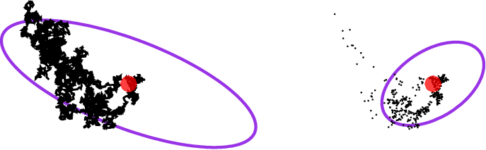
describes an ellipse whose semi-major and semi-minor axes have lengths equal to $\kappa\sqrt{\lambda_{1}}$ and $\kappa\sqrt{\lambda_{2}}$ respectively. Two examples of such ellipses are shown in Figure 1, along with the sets, $L$, of locations used to generate them.

In polymer physics, the shape of a molecule may be described by its standard gyration tensor, whose elements are the moments of its mass distribution about its centre of mass [22, 34]. The extent to which such molecules are elongated may be measured by their asphericity, which in two dimensions is defined [22]

where $\lambda_{1}$ and $\lambda_{2}$ are the eigenvalues of the gyration tensor, and the expectation is taken over all configurations of the molecule. This two dimensional asphericity is a measure of the average extent to which the ellipse defined by equation (4), departs from a circle. Since a circle is just a 1-sphere we use the terms spherical and circular interchangeably. The main focus of our paper is to explore the properties of $A_{2}$ computed from our egocentric gyration tensor (2) where the expectation is taken over the all possible sets, $L$, of memorised locations for given memory kernel. We emphasise that the egocentric version $A_{2}$ has a somewhat different interpretation to the standard $A_{2}$. Intuitively, the egocentric asphericity measures the extent to which an ellipse centred on the current location of the walker, drawn to enclose the bulk of the walker’s memory, departs from a circle. Some notable examples which illustrate the difference between the egocentric and centre–of–mass versions of $A_{2}$ are illustrated in Figure 2. As can been seen from Figures 3, 4 and 5, despite these peculiarities, the egocentric asphericity is an effective measure of the elongation of a set $L$.

The set of memory times, $S$, is a (non-homogeneous) Poisson point process on $\left[0,\infty\right)$ with intensity function $c\mu(t)$. In particular, $\mathbb{E}[|S|]=\int_{0}^{\infty}c\mu(t)dt=c$. The sums defined in (2) are taken over this process. Recall that $(X(t),Y(t))_{t\geq 0}$ is a two-dimensional standard Brownian motion. Provided the rate of memory formation is sufficiently high, we may approximate the moments of elements of $T$ by the moments of integrals with stochastic integrands, that is, for polynomials $p_{1}(x,y)=x^{2}$, $p_{2}(x,y)=y^{2}$ and $p_{3}(x,y)=xy$, as $c\to\infty$, we have

for $k\in\{1,2\}$ and $i\in\{1,2,3\}$. In particular, $\int_{0}^{\infty}p_{i}(X(s),Y(s))\mu(s)ds$ is well-defined since the distribution $\mu$ has finite first moment. For the proof of formulae (6) and (7) we refer the reader to A.

To illustrate how our egocentric asphericity theorem (Theorem 1) may be used to calculate asphericities, we work though four examples. A larger set of exact results are collected in Table 1.

To efficiently generate sample sets $S$, we make use of the fact that the set of sample times may be viewed as the arrival times of an inhomogeneous Poisson process with rate function $c\mu(t)$. At time $\tau\geq 0$, the cumulative distribution of the next arrival time $Z$ is therefore

Defining

then if $u\in[0,p(\tau))$ the inverse cumulative exists and may be written as

Note that $p(\tau)$ is the probability that there is at least one sample (arrival) time in the interval $[\tau,\infty)$. Letting the sequence of sample times be $0<Z_{1}<Z_{2}<\ldots$, then given $Z_{n}$, the next sample in memory may be simulated by noting that $Z_{n+1}\stackrel{{\scriptstyle d}}{{=}}F_{Z_{n}}^{-1}(U)$, where $\stackrel{{\scriptstyle d}}{{=}}$ denotes equality in distribution, and $U$ is a random variate uniform on $[0,1]$. The result $U>p(Z_{n})$ is equivalent to the event that $Z_{n}$ is the last sample time, and no later times are recalled. Given a simulated set, $S$, of sample times, it is straightforward to generate the set of locations $L$ by noting that

where $\mathcal{N}(\mu,\sigma^{2})$ is the normal distribution with mean $\mu$ and variance $\sigma^{2}$.

We have studied a very simple model of how a foraging animal might construct a mental map [20, 37] of its surroundings, showing that its memory kernel has a significant effect on the spatial structure of recalled locations. We have provided an analytical expression giving an egocentric version of the asphericity [22] $A_{2}$ of the set, $L$, of memory locations in terms of the memory kernel $\mu$. We have verified our analytical result by simulation, and illustrated how $A_{2}$ describes the shape of the set $L$, and how this shape is related to the tail behaviour of $\mu$. Specifically, fatter tailed kernels produce more spherical memory sets.

It has been suggested that future research into animal movement should explore the effects of memory [38, 39]. Many creatures utilise memory in order to efficiently exploit their environments [18, 19, 20, 21], and memory effects are known to effect the nature of foraging or search paths [2, 3, 17, 16, 15]. Field studies confirm that spatial memory and learning are a critical part of foraging patterns of primates [40]. Of particular relevance to the current work, is the fact that the movement of bearded saki monkeys is more consistent with Brownian motion than Lévy walk [41]. By selecting this simplest possible path model (Brownian motion), we have been able to show how these paths combine with memory to create a spatial map of the creature’s surroundings. The possession of a memory comes with physiological costs [18, 2], as does searching for food, so one would expect evolution to simultaneously optimise both paths, and the use of memory. The optimal shape and structure of a mental map will depend on the environment and objectives of the forager, so given this optimal shape, one might expect the trajectories to be influenced in part by the need to create an effective map. We therefore suggest that the search for an understanding of the relationship between trajectories, maps, and memory is worthwhile. In particular, finding the asphericity from the field data of, e.g., brearded saki monkeys or other primates forging patterns and fitting the memory kernel from our model would improve the current understanding of their spatial memory. Elaborated discussion on impact and scientific importance of mathematical modelling of movement of the foragers has been explored in [42, Part I, section 1.3].

We have used ellipses as simple approximations to the shapes of a memorised sets, but the ellipse is the simplest deformation of a circle. A natural extension is to consider higher order deformations which more accurately characterise the shape of $L$. Another possibility, which will be the subject of future research, is to consider Lévy walks and anomalous diffusions, e.g. fractional Brownian motion with Hurst parameter $H\in(0,1)\setminus\{\frac{1}{2}\}$ [43].

References

• [1] P M Kareiva and N Shigesada. Analyzing insect movement as a correlated random walk. Oecologia, 56:234–238, 1983.
• [2] W F Fagan et al. Spatial memory and animal movement. Ecol Lett, 16:1316–1329, 2013.
• [3] W F Fagan and J M Calabrese. The correlated random walk and the rise of movement ecology. Bull Ecol Soc Am, 95:204–206, 2014.
• [4] P Turchin. Quantitative Analysis of Movement. Sinauer Associates, Sunderland, MA, 1998.
• [5] E A Codling, M J Plank, and S Benhamou. Random walk models in biology. J. R. Soc. Interface, 5:8130834, 2008.
• [6] S L Collins et al. New opportunities in ecological sensing using wireless sensor networks. Front. Ecol. Environ., 4:402–407, 2006.
• [7] E P Raposo et al. Dynamical robustness of Lévy search strategies. Phys. Rev. Lett., 91:240601, 2003.
• [8] A James, M J Plank, and A M Edwards. Assessing Lévy walks as models of animal foraging. J. R. Soc. Interface, 8:233–1247, 2011.
• [9] G M Viswanathan, E P Raposo, and M G E da Luz. Lévy flights and superdiffusion in the context of biological encounters and random searches. Phys. Life Rev., 5:133–150, 2008.
• [10] G M Viswanathan et al. Optimizing the success of random searches. Nature, 401:911–914, 1999.
• [11] N E Humphries et al. Environmental context explains Lévy and Brownian movement patterns of marine predators. Nature, 465:1066–1069, 2010.
• [12] G F Lawler. Introduction to stochastic processes. CRC Press, Boca Raton, FL, 2006.
• [13] J D Thomson. Trapline foraging by bumblebees: I. persistence of flight-path geometry. Behav. Ecol., 7:158–164, 1996.
• [14] F B Gill. Trapline foraging by hermit hummingbirds: Competition for an undefended, renewable resource. Ecology, 69:1933–1942, 1988.
• [15] K Ohashi and J D Thomson. Efficient harvesting of renewing resources. Behav. Ecol., 16:592–605, 2005.
• [16] D Boyer and C Solis-Salas. Random walks with preferential relocations to places visited in the past and their application to biology. Phys. Rev. Lett., 112:240601, 2014.
• [17] D Boyer, M C Crofoot, and P D Walsh. Non-random walks in monkeys and humans. J. R. Soc. Interface, 9:842–847, 2012.
• [18] R Dukas. Costs of memory ideas and predictions. J. theor. Biol., 197:41–50, 1999.
• [19] T C Roth, N C Rattenborg, and V V Pravosudov. The ecological relevance of sleep: the trade-off between sleep, memory and energy conservation. Phil. Trans. R. Soc. B, 365:945–959, 2010.
• [20] E Normand and C Boesch. Sophisticated euclidean maps in forest chimpanzees. Animal Behav., 77:1195–1201, 2009.
• [21] T Avgar, A Mosser, G S Brown, and J M Fryxell. Environmental and individual drivers of animal movement patterns across a wide geographical gradient. J. Animal Ecol., 82:96–106, 2012.
• [22] J Rudnick and G Gaspari. The asphericity of random walks. J. Phys. A: Math. Gen., 19:L191–L193, 1986.
• [23] L Avrell and A Heathcote. The form of the forgetting curve and the fate of memories. J. Math. Psychol., 55:25–35, 2011.
• [24] G Claussen, A K Hartmann, and S N Majumdar. Convex hulls of random walks: Large-deviation properties. Phys. Rev. E, 91:052104, 2015.
• [25] D S Grebenkov, Y Lanoiselée, and S N Majumdar. Mean perimeter and mean area of the convex hull over planar random walks. J. Stat. Mech., 2017:103203, 2017.
• [26] B Øksendal. Stochastic Differential Equations: An Introduction with Applications. Springer, Berlin, 2010.
• [27] V Mendez, D Campos, and F Bartumeus. Stochastic Foundations in Movement Ecology. Springer, 2014.
• [28] E Bénichou and S Redner. Depletion-controlled starvation of a diffusing forager. Phys. Rev. Lett, 113:238101, 2014.
• [29] E Bénichou, U Bhat, P L Krapivsky, and S Redner. Optimally frugal foraging. Phys. Rev. E, 97:022110, 2018.
• [30] U Bhat, S Redner, and E Bénichou. Does greed help a forager survive? Phys. Rev. E, 95:062119, 2017.
• [31] C E Vincenot et al. How spatial resource distribution and memory impact foraging success: A hybrid model and mechanistic index. Ecol. Complex., 22:139–151, 2015.
• [32] C Bracis, E Gurarie, B van Moorter, and A Goodwin. Memory effects on movement behavior in animal foraging. PLoS ONE, 10:e0136057, 2015.
• [33] R L Klatzky. Allocentric and Egocentric Spatial Representations: Definitions, Distinctions, and Interconnections Spatial Cognition (Lecture Notes in Computer Science vol 1404), volume 1404. Springer, 1998.
• [34] J Rudnick, A Beldjenna, and G Gaspari. The shapes of high-dimensional random walks. J. Phys. A: Math. Gen., 20:971–984., 1987.
• [35] G Grimmett and D Stirzaker. Probability and Random Processes. Oxford University Press, Oxford, 2001.
• [36] F W J Olver, D W Lozier, R F Boisvert, and C W Clark. NIST Handbook of Mathematical Functions. Cambridge University Press, 2010.
• [37] C H Janson. Experimental evidence for spatial memory in foraging wild capuchin monkeys, cebus apella. Animal Behav., 55:1229–1243, 1998.
• [38] J M Morales et al. Extracting more out of relocation data: building movement models as mixtures of random walks. Ecology, 85:2436–2445, 2004.
• [39] T A Patterson et al. State-space models of individual animal movement. Trends Ecol Evol., 23:87–94, 2008.
• [40] P A Garber. Role of spatial memory in primate foraging patterns: Saguinus mystax and saguinus fuscicollis. Am. J. Primatol., 19:203–216, 1989.
• [41] C A Shaffer. Spatial foraging in free ranging bearded sakis: traveling salesmen or Lévy walkers? Am. J. Primatol., 76:472–84, 2014.
• [42] G M Viswanathan, M G E da Luz, E P Raposo, and Stanley H E. The Physics of Foraging. An Introduction to Random Searches and Biological Encounters. Cambridge University Press, Cambridge, 2011.
• [43] F Biagini, Y Hu, and Øksendal B. Stochastic Calculus for Fractional Brownian Motion and Applications. Springer, Berlin, 2008.
• [44] R L Streit. Poisson Point Processes. Imaging, Tracking, and Sensing. Springer, 2010.
• [45] J F C Kingman. Poisson Processes. Clarendon Press, Oxford, 2002.
• [46] F Baccelli and P Bremaud. Elements of Queueing Theory. Palm Martingale Calculus and Stochastic Recurrences. Springer, Berlin, 2002.