Steady-state generation of Wigner-negative states in 1D resonance fluorescence
Abstract
In this work we demonstrate numerically that the nonlinearity provided by a continuously driven two-level system (TLS) allows for the generation of Wigner-negative states of the electromagnetic field confined in one spatial dimension. Wigner-negative states, a.k.a. Wigner nonclassical states, are desirable for quantum information protocols beyond the scope of classical computers. Focusing on the steady-state emission from the TLS, we find the largest negativity at the drive strength where the coherent reflection vanishes.
Introduction.—
In this Letter we present the calculation of the Wigner function of one-dimensional (D) steady-state resonance fluorescence. Resonance fluorescence, the spontaneous emission from a two-level system (TLS) driven by a resonant electromagnetic field [1], is one of the simplest theoretical models for studying the light-matter interaction. Despite its basic structure, this model exhibits very rich phenomena, including photon antibunching [2], squeezing in the scattered field of a very weak drive [3], and an inelastic scattering spectrum (Mollow triplet) for a strong drive [4].
The Wigner function [5, 6, 7], a quasi-probability distribution which allows for a description of quantum mechanics in phase space, recently gathered relevance in the context of continuous variable (CV) quantum information [8, 9]. This is because it allows to discern the class of states necessary for achieving a quantum advantage over classical simulations. This class corresponds to Wigner-negative states, i.e, states characterized by a negative Wigner function [10, 11, 12]. Assuming a coherent drive, a nonlinearity is required in order to generate Wigner negativity.
The TLS is a nonlinear medium interacting with the incoming radiation, causing the reflection (transmission) to be dependent on the intensity of the radiation. In order to avoid a spatial mode mismatch between incoming and scattered fields, it is desirable to confine the emission to a single spatial dimension. Artificial 1D systems provide an ideal testbed for studying the light-matter interaction due to its enhancement as a consequence of the confinement [13, 14, 15, 16, 17, 18, 19].
Here we study the resonant scattering from a TLS in front of a mirror. The mirror serves two purposes. First, it avoids the loss of information due to an unobserved channel: a transmitted component. Second, and more important, it has been demonstrated that in this configuration it is possible to cancel the coherent component of the scattered field [20, 21]. It is known that this setup allows for single-photon generation when the TLS is driven with a pulse. Prominent examples of this are superconducting circuits [22, 23, 24, 25] and quantum dot [26, 27, 28, 29] setups. Single photons have no classical counterpart and are correspondingly characterized by a negative Wigner function. Still, the question of steady-state emission from a continuously driven TLS remains. In contrast to the pulsed scheme for which the exponential decay of the TLS gives a known probability of detecting the emitted photon in time, we lack this information when driving continuously. The uncertainty in the emission time of the photon enhances the role of the vacuum in the emitted state. Additionally, Fock states other than the vacuum and a single-photon may contribute to the output field. In this Letter we explore if the nonlinearity of a continuously driven TLS suffices to generate Wigner nonclassical states of light. Furthermore, in contrast to nondeterministic nonlinear operations commonplace in quantum optics such as photon substraction [30] or cubic phase gate approximations [31, 32, 33], we explore steady-state and deterministic generation of this class of states.
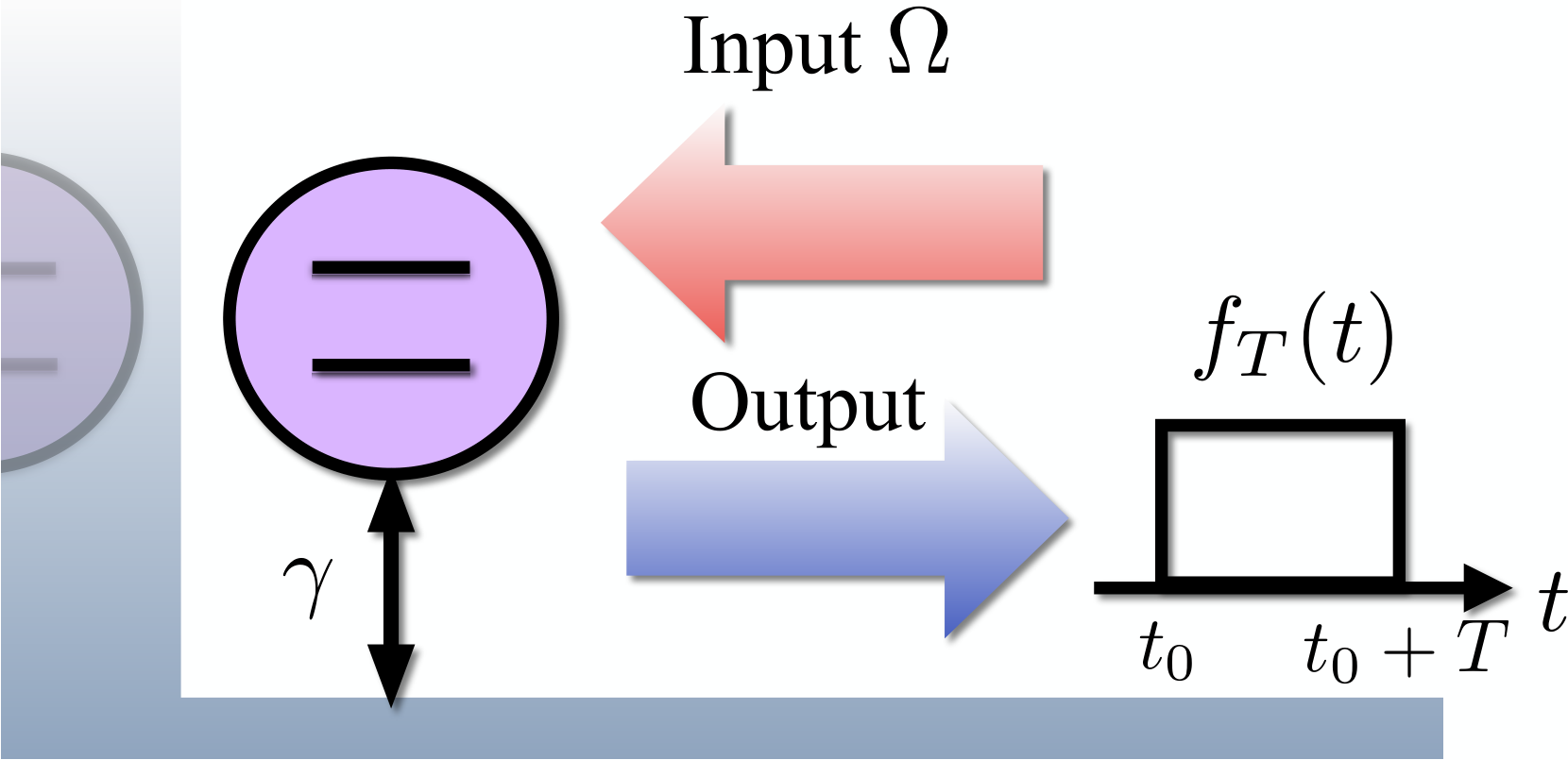
We use quantum trajectories [34, 35] together with Maximum Likelihood estimation [36, 37] in order to reconstruct the state and Wigner function of the scattered field. We study under which conditions this field is characterized by a negative Wigner function, and furthermore, quantify its negativity content.

The setup.—
In the absence of a mirror, the scattered radiation from a TLS coupled to a 1D continuum contains both reflected and transmitted components. The role of the mirror is to restrict the emission into a single (reflected) component. The distance between the TLS and the mirror is crucial [21, 38]. A non-zero separation results in time-delay effects which lead to non-Markovian dynamics [38]. In this work, we assume that the TLS-mirror separation is negligible.
A TLS driven by a resonant coherent field of amplitude is described in the rotating frame of the drive by the Hamiltonian (we set hereafter)
| (1) |
where is the incoming power and () is the TLS lowering (raising) operator. Here is the coupling strength to the environment—the electromagnetic field confined in D— which contains both the incoming coherent drive and the output field.
Considering the environment as a reservoir at zero temperature, the dissipative dynamics of the TLS is described by the quantum master equation
| (2) |
This setup is sketched in Fig. 1.
The behavior of a TLS in front of a mirror can be understood by studying the two-time correlations of the output field [39]
| (3) |
From the steady-state of (2) (), it is straightforward to derive the correlation function
| (4) |
where the subscript ss indicates that expectation values are calculated in the steady-state. Here is a function of and which we do not write explicitly for the sake of simplicity (see Supplementary Material [40]). The time-independent part of (4) corresponds to , i.e., a coherent state. In both the weak () and strong () driving regimes, this is the dominant part of the field, i.e., . For a TLS in front of a mirror there is a drive strength for which [21]. From (4) we find that . For this drive strength, the first term on the right-hand-side of (4) is equal to zero, and we only retain the time-dependent terms, meaning the response of the system is entirely incoherent. We will refer to as the incoherent drive point. A coherent state is a Gaussian state, and is therefore characterized by a positive Wigner function [41]. Thus, in order to witness Wigner nonclassicality we focus on the drive strength for which the coherent response is supressed.
Filtered modes.—
The Wigner function is defined for a single bosonic mode [6]. However, the field interacting with the TLS is a propagating field and corresponds to a continuum of modes in time (or frequency). In order to construct the Wigner function we need to pick a single mode out of this continuum. Following [42], this can be done using a filter function. We define the filtered creation operator
| (5) |
If the filter function satisifies the normalization condition , then the field obeys the bosonic commutation relation .
For simplicity, we choose to filter the steady-state emission with a boxcar filter [Cf. Fig. 1]
| (6) |
which is a constant function within the time interval from to and zero elsewhere. Here represents the time at which the measurement starts and is the Heaviside step function. The filter time defines the only time scale in our problem. The Fourier transform of a boxcar filter (6) in time is a sinc function in frequency space. Correspondingly, the filter imposes an approximate bandwidth of —the width of the sinc central peak.
The filter function defines what is the observed mode upon tomography. We have also carried out the simulations presented in the next section using a Gaussian filter and the results are essentially the same.
Witnessing Wigner negativity.—
Homodyne tomography is an experimental technique which allows to reconstruct the Wigner function of an arbitrary state of light [36]. This relies on homodyne detection [37], i.e., the measurement of the generalized quadrature operators , with . The quantum state is then inferred from the measurement statistics. Using quantum trajectories [34, 35], we numerically simulate the conditional evolution of the TLS which results from its emission being subjected to homodyne detection. The TLS is initialised in its ground state and the measurements are taken from a large time [Cf. Eq. (6)] in which the (unconditional) master equation (2) has reached the stationary state. From the quadrature measurement statistics the state of the field is reconstructed by means of Maximum Likelihood estimation [36, 37]. Technical details can be found in [40, 43]. Knowing the state of the field, it is straightforward to calculate its Wigner function [44]. We will focus on the emission from the TLS, that is, we will ignore the reflected drive field in (3). The effect of the latter is to displace the field emitted by the TLS. This operation corresponds to a translation of the Wigner function in phase space, which does not affect its negativity [40].
In Fig. 2 we show the Wigner function of the output field from the TLS in front of a mirror, driven with strength , for four different filter times and (in units of ). As can be expected based on the discussion after Eq. (4), at the incoherent drive point the output field is nonclassical as manifested by a negative Wigner function (Fig. 4(b) and (c)). This is the main result of this Letter.
In Fig. 3 we show the populations of the photon number states and as a function of the filter time at the incoherent drive point. In this figure we compare the populations for the reconstructed states from our quantum trajectory simulations with analytical solutions for the total, unfiltered, output field. The unfiltered field corresponds to the infinite bandwidth limit and its photon number content can be calculated analytically [45, 24]. For , there is an agreement between both solutions. This is no longer the case for larger values of . As discussed in the previous section, the boxcar filter introduces an effective bandwidth of . Therefore, as we approach the infinite bandwidth limit () both solutions agree with each other. By increasing the filter time, we reduce the effective bandwidth and we are not able to detect all of the emitted photons. In addition, for filter times , two-photon states can safely be neglected in the output field (they constitute less than of the total population). In the following, we study the origin of negativity in a Wigner function restricted to a two-dimensional Fock space.
The most general state in the space spanned by the vacuum and a single-photon is of the form , with the normalization condition . The Wigner function of is [44]
| (7) |
with the Wigner function of a Fock state () [7], and the th order Laguerre polynomial. In order to quantify the presence of Wigner negativity we use the total integrated negativity [46, 47, 48], defined as
| (8) |
This is a measure of the volume of the negative part of the Wigner function, such that .
In a two-dimensional Fock space, the presence of negativity () is determined by the populations and . However, the specific relation between them for a state to be Wigner-negative is set by the coherences , or equivalently, by the purity of the state. For a pure state a very small single-photon population () is enough for the Wigner function to be negative. This negativity content is enhanced by increasing . As the purity of the state decreases, the condition for it to be Wigner-negative is roughly . The exact relation between and depends on the particular value of the purity. For an incoherent mixture of and , i.e., , the condition becomes .
This analysis is important, as in general the output state from an atom in front of a mirror is mixed. In fact, the output state is pure only in the limit of very weak or strong driving. Following our discussion on two-time correlations of the output field, in both regimes the output is a coherent state. Away from the strong driving regime, the purity of the output field decreases with an increasing drive [40].
At the incoherent drive point, from Fig. 3 it follows that near , the vacuum and single-photon contributions to the state become identical. Following our previous discussion, it is around this point where we expect the Wigner function to become negative as the state is mixed [40]. To verify this, we calculate the total integrated negativity. However, to get a feeling for the magnitude of this quantity, instead of presenting the negativity (8) we show the relative negativity . We define the latter as the ratio between the total integrated negativity of our state and the total integrated negativity of a single photon : . In Fig. 4 we show the relative negativity as a function of for different drive strengths. For (open black squares in Fig. 4) we see that there is a correspondence between an increasing single-photon population [Cf. Fig. 3] and the appearance of negativity. The maximum negativity occurs around , and the corresponding Wigner function is shown in Fig. 2 (c). Here, the two-photon population is no longer negligible. Nevertheless, it is still the dominant single-photon contribution which renders the state Wigner-negative. In fact, using the general expression for the Wigner function of a Fock state (given below Eq. (7)), it can be shown that a small population of reduces the negativity contribution of in a mixed state. Therefore, it is the increasing two-photon population which stops the negativity from growing further. For longer filter times (), decreases to zero. Here, higher number states are also involved and the analysis is not straightforward. It is worth to emphasize that we observe Wigner negativity beyond mixtures of vacuum and single-photons.
We have verified that the largest negativity achieved for the output field occurs at . In Fig. 4, we compare the relative negativity for different drive strengths in order to show the observed characteristic behavior. For (filled red diamonds and open green circles in Fig. 4), the output state is also mixed and therefore, using the two-dimensional Fock space approximation, the state becomes negative whenever . The corresponding populations are shown in [40]. Also for drive strengths , the approximation of a two-dimensional Fock space breaks down at smaller values of compared to the incoherent drive point. This means that the single-photon population becomes dominant at a shorter filter time , which explains the shift in the position of the maximum towards smaller for stronger drives. In these cases, the enhanced presence of higher number states () in the output notably reduces the maximum negativity achieved.
The case (filled blue squares in Fig. 4), is different because the state is almost pure. Following the discussion after Eq. (8), a smaller single-photon population suffices for the state to become negative. Consequently, the transition from zero to non-zero negativity is less sharp than for . For the same reason, negativity is present for a larger range of values of compared to stronger drives.
In Ref. [18], the authors calculate the Wigner function of resonance fluorescence analytically in order to explain the phase-dependent nature of squeezing. We believe that their approach, mapping the steady-state of the TLS into the field, does not correspond to steady-state emission. It is however correct if the drive is switched off once the steady-state is reached and the emission from the TLS is homodyned with a filter matching its decay in time.
The setup presented in this Letter is already experimentally feasible. Most notable realizations are found in superconducting circuits and quantum dots. In superconducting circuits, a measurement scheme closely resembling homodyne detection corresponds to phase sensitive amplification [49]. Alternatively, there are other schemes for characterizing propagating fields [50, 51, 22, 52, 53]. Quantum state tomography for the scattering of coherent states on an array of quantum dots has already been reported [54].
Conclusions.—
We have calculated the Wigner function of D resonance fluorescence from a TLS in front of a mirror. We use the mirror to exactly cancel the coherent emission from the TLS. We have shown that at the incoherent drive point the Wigner function achieves its maximum negativity content.
Protocols have been demonstrated where, e.g., the cubic phase gate, which allows to promote the Gaussian set of gates to a universal set [9], can be obtained by using input non-Gaussian ancillary states together with Gaussian operations and measurements [33, 55]. Therefore, we have verified that this simple setup suffices to generate the class of states necessary for universal quantum computing beyond the scope of classical computers.
Acknowledgments.—
The authors would like to thank Giulia Ferrini, Sankar Raman Sathyamoorthy, Adam Miranowicz, Sahin K. Özdemir and Steven Girvin for valuable discussions. FQ and GJ acknowledge the support from the Knut and Alice Wallenberg Foundation. IS acknowledges the support from Chalmers Excellence Initiative Nano.
References
- [1] D. Walls and G. Milburn, Quantum Optics (Springer Berlin Heidelberg, 2008).
- [2] H. J. Kimble, M. Dagenais, and L. Mandel, Phys. Rev. Lett. 39, 691 (1977).
- [3] D. F. Walls and P. Zoller, Phys. Rev. Lett. 47, 709 (1981).
- [4] B. R. Mollow, Phys. Rev. 188, 1969 (1969).
- [5] E. Wigner, Phys. Rev. 40, 749 (1932).
- [6] M. Hillery, R. O’Connell, M. Scully, and E. Wigner, Physics Reports 106, 121 (1984).
- [7] C. Gardiner and P. Zoller, Quantum Noise, Springer Series in Synergetics (Springer, 2004).
- [8] S. Lloyd and S. L. Braunstein, Phys. Rev. Lett. 82, 1784 (1999).
- [9] M. Gu, C. Weedbrook, N. C. Menicucci, T. C. Ralph, and P. van Loock, Phys. Rev. A 79, 062318 (2009).
- [10] A. Mari and J. Eisert, Phys. Rev. Lett. 109, 230503 (2012).
- [11] V. Veitch, N. Wiebe, C. Ferrie, and J. Emerson, New Journal of Physics 15, 013037 (2013).
- [12] S. Rahimi-Keshari, T. C. Ralph, and C. M. Caves, Phys. Rev. X 6, 021039 (2016).
- [13] D. E. Chang, A. S. Sørensen, E. A. Demler, and M. D. Lukin, Nature Physics 3, 807 (2007).
- [14] A. Muller, E. B. Flagg, P. Bianucci, X. Y. Wang, D. G. Deppe, W. Ma, J. Zhang, G. J. Salamo, M. Xiao, and C. K. Shih, Phys. Rev. Lett. 99, 187402 (2007).
- [15] O. Astafiev, A. M. Zagoskin, A. A. Abdumalikov, Y. A. Pashkin, T. Yamamoto, K. Inomata, Y. Nakamura, and J. S. Tsai, Science 327, 840 (2010).
- [16] B. Peropadre, J. Lindkvist, I.-C. Hoi, C. M. Wilson, J. J. Garcia-Ripoll, P. Delsing, and G. Johansson, New Journal of Physics 15, 035009 (2013).
- [17] I.-C. Hoi, C. M. Wilson, G. Johansson, T. Palomaki, B. Peropadre, and P. Delsing, Phys. Rev. Lett. 107, 073601 (2011).
- [18] C. H. H. Schulte, J. Hansom, A. E. Jones, C. Matthiesen, C. Le Gall, and M. Atatüre, Nature (London) 525, 222 (2015).
- [19] X. Gu, A. F. Kockum, A. Miranowicz, Y. xi Liu, and F. Nori, Physics Reports 718-719, 1 (2017), microwave photonics with superconducting quantum circuits.
- [20] K. Koshino and Y. Nakamura, New Journal of Physics 14, 043005 (2012).
- [21] I.-C. Hoi, A. F. Kockum, L. Tornberg, A. Pourkabirian, G. Johansson, P. Delsing, and C. M. Wilson, Nature Physics 11, 1045 (2015).
- [22] C. Eichler, D. Bozyigit, C. Lang, M. Baur, L. Steffen, J. M. Fink, S. Filipp, and A. Wallraff, Phys. Rev. Lett. 107, 113601 (2011).
- [23] Y. Yin, Y. Chen, D. Sank, P. J. J. O’Malley, T. C. White, R. Barends, J. Kelly, E. Lucero, M. Mariantoni, A. Megrant, C. Neill, A. Vainsencher, J. Wenner, A. N. Korotkov, A. N. Cleland, and J. M. Martinis, Phys. Rev. Lett. 110, 107001 (2013).
- [24] S. R. Sathyamoorthy, A. Bengtsson, S. Bens, M. Simoen, P. Delsing, and G. Johansson, Phys. Rev. A 93, 063823 (2016).
- [25] P. Forn-Díaz, C. W. Warren, C. W. S. Chang, A. M. Vadiraj, and C. M. Wilson, Phys. Rev. Applied 8, 054015 (2017).
- [26] C. Matthiesen, A. N. Vamivakas, and M. Atatüre, Phys. Rev. Lett. 108, 093602 (2012).
- [27] Y.-M. He, Y. He, Y.-J. Wei, D. Wu, M. Atatüre, C. Schneider, S. Höfling, M. Kamp, C.-Y. Lu, and J.-W. Pan, Nature Nanotechnology 8, 213 (2013).
- [28] P. Lodahl, S. Mahmoodian, and S. Stobbe, Rev. Mod. Phys. 87, 347 (2015).
- [29] X. Ding, Y. He, Z.-C. Duan, N. Gregersen, M.-C. Chen, S. Unsleber, S. Maier, C. Schneider, M. Kamp, S. Höfling, C.-Y. Lu, and J.-W. Pan, Phys. Rev. Lett. 116, 020401 (2016).
- [30] M. S. Kim, Journal of Physics B: Atomic, Molecular and Optical Physics 41, 133001 (2008).
- [31] M. Yukawa, K. Miyata, H. Yonezawa, P. Marek, R. Filip, and A. Furusawa, Phys. Rev. A 88, 053816 (2013).
- [32] K. Marshall, R. Pooser, G. Siopsis, and C. Weedbrook, Phys. Rev. A 91, 032321 (2015).
- [33] F. Arzani, N. Treps, and G. Ferrini, Phys. Rev. A 95, 052352 (2017).
- [34] H. Wiseman and G. Milburn, Quantum Measurement and Control (Cambridge University Press, 2010).
- [35] T. A. Brun, American Journal of Physics 70, 719 (2002).
- [36] A. I. Lvovsky, Journal of Optics B: Quantum and Semiclassical Optics 6, S556 (2004).
- [37] A. I. Lvovsky and M. G. Raymer, Rev. Mod. Phys. 81, 299 (2009).
- [38] H. Pichler and P. Zoller, Phys. Rev. Lett. 116, 093601 (2016).
- [39] C. W. Gardiner and M. J. Collett, Phys. Rev. A 31, 3761 (1985).
- [40] See supplementary material in this submission.
- [41] R. Hudson, Reports on Mathematical Physics 6, 249 (1974).
- [42] R. Loudon, The quantum theory of light, Oxford science publications (Clarendon Press, 1983).
- [43] I. Strandberg, Quantum state tomography of 1D resonance fluorescence, Master’s thesis, Chalmers University of Technology (2017).
- [44] J. E. Moyal and M. S. Bartlett, Proceedings of the Cambridge Philosophical Society 45, 99 (1949).
- [45] J. Lindkvist and G. Johansson, New Journal of Physics 16, 055018 (2014).
- [46] A. Kenfack and K. Życzkowski, Journal of Optics B: Quantum and Semiclassical Optics 6, 396 (2004).
- [47] F. Albarelli, A. Ferraro, M. Paternostro, and M. G. A. Paris, Phys. Rev. A 93, 032112 (2016).
- [48] C. Joana, P. van Loock, H. Deng, and T. Byrnes, Phys. Rev. A 94, 063802 (2016).
- [49] F. Mallet, M. A. Castellanos-Beltran, H. S. Ku, S. Glancy, E. Knill, K. D. Irwin, G. C. Hilton, L. R. Vale, and K. W. Lehnert, Phys. Rev. Lett. 106, 220502 (2011).
- [50] E. P. Menzel, F. Deppe, M. Mariantoni, M. A. Araque Caballero, A. Baust, T. Niemczyk, E. Hoffmann, A. Marx, E. Solano, and R. Gross, Phys. Rev. Lett. 105, 100401 (2010).
- [51] M. P. da Silva, D. Bozyigit, A. Wallraff, and A. Blais, Phys. Rev. A 82, 043804 (2010).
- [52] E. P. Menzel, R. Di Candia, F. Deppe, P. Eder, L. Zhong, M. Ihmig, M. Haeberlein, A. Baust, E. Hoffmann, D. Ballester, K. Inomata, T. Yamamoto, Y. Nakamura, E. Solano, A. Marx, and R. Gross, Phys. Rev. Lett. 109, 250502 (2012).
- [53] K. G. Fedorov, L. Zhong, S. Pogorzalek, P. Eder, M. Fischer, J. Goetz, E. Xie, F. Wulschner, K. Inomata, T. Yamamoto, Y. Nakamura, R. Di Candia, U. Las Heras, M. Sanz, E. Solano, E. P. Menzel, F. Deppe, A. Marx, and R. Gross, Phys. Rev. Lett. 117, 020502 (2016).
- [54] F. Boehm, N. B. Grosse, M. Kolarczik, B. Herzog, N. Owschimikow, and U. K. Woggon, in Nonlinear Optics (Optical Society of America, 2017) p. NTh2A.1.
- [55] F. Albarelli, M. G. Genoni, M. G. A. Paris, and A. Ferraro, ArXiv e-prints (2018), arXiv:1804.05763 [quant-ph] .
Appendix A Two-time correlation functions in the steady-state
The steady-state (ss) two-time correlation (Eq. (4) in the main text), can be related to correlations of the TLS lowering and raising operators by the input-output relation (Eq. (3) in the main text). In this way, we have
| (9) |
The first step is to solve for the vector in the steady-state. The solutions are
| (10) | ||||
| (11) |
From here, the two-time correlation of the TLS operators can be calculated by using the quantum regression theorem [1]. The result is
| (12) |
with
| (13) |
Inserting (10) and (12) in (9) yields Eq. (3) in the main text.
Appendix B Wigner function of a displaced state
The Wigner function of a state is defined as [6]
| (14) |
We now introduce the (unitary) displacement operator on a bosonic mode annihilated (created) by () satisfying the commutation relation
| (15) |
Its action on the annihilation operator is defined by
| (16) |
We can rewrite (15) in terms of the quadrature operators and :
| (17) |
Its action on the position quadrature eigenstates () is
| (18) |
The displaced state is defined by
| (19) |
Following the definition (14), the Wigner function of the displaced state is
| (20) |
Using relation (18), this reduces to
| (21) |
Comparing (14) and (21), we see that they are related by a translation, i.e., we go from (21) to (14) by shifting the origin of phase space from to . The Wigner function is simply displaced by .
Appendix C Purity
In Fig. 5 we show the purity of the filtered output field as a function of the filter time and for drive strengths , 0.35, 0.5 and 0.8 (in units of ). These correspond to the states studied in the main text [Cf. Fig. (4)].
Appendix D Photon populations
In Figs. 6, 7 and 8 we show the photon populations in the filtered output field as a function of the filter time and for drive strengths , 0.5 and 0.8 (in units of ). These populations correspond to the states studied in the main text [Cf. Fig. (4)].
Appendix E Maximum Likelihood
The goal of homodyne tomography is to infer the state of a single bosonic mode with . In a homodyne detection experiment, the measured quantity is the photocurrent, which is proportional to the expectation value of the generalized quadrature observable
| (22) |
with a real phase. The quadrature operator is a continuous variable with eigenstates corresponding to the eigenvalues , i.e., .
Homodyne detection is a diffusive type of measurement dominated by Gaussian noise. For a fixed value of , through repeated measurements we can estimate the quadrature probabilities . From this data, the state can be inferred via Maximum Likelihood estimation [37].
Since is a continuous variable and the total number of measurements is finite, the data must be binned. In order to do this, we split a relevant domain of the real axis into intervals . From here, the binned quadrature probabilities, for fixed , are obtained by integration as
| (23) |
Maximum Likelihood is a statistical inference method. The idea is to search for the physical state which maximizes the probability of obtaining the measured quadrature probabilities.
For an arbitrary state , we define the likelihood function
| (24) |
with the number of measurements in the -th bin, i.e., the binned histogram. The latter is related to the actual state we are trying to infer. The goal is to find the state which maximizes the likelihood function. This state will be our best approximation to .
The state which maximizes the likelihood obeys the extremal equation
| (25) |
with the state-dependent operator defined as
| (26) |
Here is the total number of measurements for a fixed phase , is the total number of measurements and the projector into the -th bin
| (27) |
The extremal condition (25) amounts to being proportional to the identity operator. Indeed, for the probability equals the -th entry of the normalized measurement histogram , and therefore, we are left with a sum of projectors over the different bins. Following Eq. (27), the sum is equal to the identity operator.
The state which maximizes the likelihood function can be found iteratively. First, we choose a basis in which to represent the density matrix. In our case, this will be the Fock or number basis with a photon number cutoff . Then, starting from an arbitrary state, in our case , the iterative search proceeds as follows
| (28) |
where denotes normalization to unity trace. We stop the iterations when the variation in the state, quantified by a suitable norm, for consecutive iterations is sufficiently small. In our case,
| (29) |
The chosen matrix norm is the Frobenius norm, defined as for a matrix .