Post model-fitting exploration via a “Next-Door” analysis
Abstract
We propose a simple method for evaluating the model that has been chosen by an adaptive regression procedure, our main focus being the lasso. This procedure deletes each chosen predictor and refits the lasso to get a set of models that are “close” to the one chosen, referred to as “base model”. If the deletion of a predictor leads to significant deterioration in the model’s predictive power, the predictor is called indispensable; otherwise, the nearby model is called acceptable and can serve as a good alternative to the base model. This provides both an assessment of the predictive contribution of each variable and a set of alternative models that may be used in place of the chosen model.
In this paper, we will focus on the cross-validation (CV) setting and a model’s predictive power is measured by its CV error, with base model tuned by cross-validation. We propose a method for comparing the error rates of the base model with that of nearby models, and a p-value for testing whether a predictor is dispensable. We also propose a new quantity called model score which works similarly as the p-value for the control of type I error. Our proposal is closely related to the LOCO (leave-one-covarate-out) methods of (Rinaldo et al. (2016)) and less so, to Stability Selection (Meinshausen & Bühlmann (2010)).
We call this procedure “Next-Door analysis” since it examines models close to the base model. It can be applied to Gaussian regression data, generalized linear models, and other supervised learning problems with penalization. It could also be applied to best subset and stepwise regression procedures. We have implemented it in the R language as a library to accompany the well-known glmnet library.
1 Introduction
We consider the usual regression or classification situation: we have samples , where and are the regressors and response for the observation. In regression, is quantitative while in classification it takes on one of discrete values. We will focus for now on the regression problem, but will discuss classification in Section 5.
We assume that an adaptive regression procedure has been fit to the data, and we want to assess the chosen model(base model). Our main focus in this paper is on the lasso, although procedures such as subset or stepwise regression may also be amenable to our approach. The lasso method solves the following problem(for simplicity, we have left out the intercept):
| (1) |
yielding a final model with sparse coefficients , for a sufficiently large value of . The data analyst is often interested in the importance of the selected predictors.
One way to measure the importance is to adopt a sub-model interpretation where we consider whether a predictor has a non-zero coefficient in the selected model. Conditional on the selected model, we can form post-selection p-values for the non-zero coefficients (Berk et al. (2013); Lee & Taylor (2014); Lee et al. (2016); Tibshirani et al. (2016); Tibshirani et al. (2015); Fithian et al. (2014)). Another way to measure its importance is to consider if the deletion of this predictor leads to significant deterioration in the predictive power given a training procedure. If the answer is “yes”, this predictor is indispensable. Otherwise, the new model trained without this feature is acceptable and may work as a substitute for the base model.
The measures coincide when there is no feature selection. When , we can fit a full regression model
If we restrict ourselves to the OLS regression only, the p-value that we obtain for each predictor reflects both (1) the significance of its coefficient being non-zero conditional in the current model, and (2) the deterioration in predictive power when the predictor is deleted and the model is refitted. When is large and especially when , a full regression fit is not feasible, and the lasso is a popular approach for fitting. When we use the lasso penalty to select a model, however, these two criteria are different. The recent progress in the field of post selection inference has focused on the sub-model interpretation. In practice, researchers will sometimes be more interested in the second perspective.
Motivated by the discussion above, we propose to find and assess models “close” to the base model, a procedure that we call Next-Door analysis. The idea is as follows. We first fit the usual lasso, using cross-validation to choose . Then for each predictor in the support set, we remove that predictor and refit the lasso to all of the remaining predictors (not just the support set) using the chosen value of . This gives a nearby model(proximal model) corresponding to the deletion of each of the member of support set. Finally, we examine and evaluate each of these nearby models. Algorithm 1 gives the details.
Algorithm 1: Next-Door analysis for the lasso
- 1.
Fit the lasso with parameter chosen by cross-validation. Let the solution be . Let be the active set where the coefficient in is non-zero.
- 2.
For each , solve the lasso problem with the coefficient for the predictor being fixed at 0:
(2) Let be the increase in the true validation error for this model relative to the base model.
- 3.
Form an unbiased estimate of and test if predictor is indispensable: that is, test whether is positive.
As outlined in Algorithm 1, our test for indispensibiltiy is a test of . It is challenging since the candidate models and the hypothesis are data adaptive and involve selections. One main task of this paper is to provide a good estimate of the p-value for the above test taking into consideration the selections.
. base lcavol lweight svi lcp lbph pgg45 age lcavol 0.64 0.69 0.70 0.59 0.65 0.63 0.62 lweight 0.27 0.37 0.30 0.27 0.35 0.27 0.26 svi 0.25 0.46 0.29 0.22 0.21 0.27 0.25 lcp -0.12 0.07 -0.11 -0.01 -0.14 -0.04 -0.11 lbph 0.18 0.21 0.29 0.14 0.19 0.18 0.17 pgg45 0.17 0.18 0.13 0.19 0.13 0.18 0.15 age -0.08 -0.02 -0.03 -0.09 -0.07 -0.05 -0.07 gleason 0.07 0.07 cv_error 0.61 0.90 0.65 0.64 0.62 0.61 0.63 0.60 debiased_error 0.62 0.94 0.66 0.66 0.63 0.62 0.62 0.62 test_error 0.51 0.87 0.49 0.56 0.50 0.50 0.47 0.53 selection frequency 1.00 1.00 0.96 0.78 1.00 0.88 0.74 model pvalue 0.01 0.21 0.20 0.29 0.48 0.26 0.34 model score 0.01 0.21 0.21 0.37 0.48 0.30 0.45 feature pvalue 0.00 0.01 0.02 0.23 0.05 0.07 0.28
Table 1 gives a preview of results from a Next-Door analysis. We apply it to a prostate cancer data set taken from Friedman et al. (2001). The data consists of training observations and 30 test observations. There are eight predictors. The response is the log PSA for men who had prostate cancer surgery. Each column contains one set of model coefficients using a fixed training procedure. The columns corresponding to the proximal models are ordered according to their de-biased CV errors(from small to large). Details of the model p-value and model score for the “indispensability test” are provided in Section 2. The “selection frequency” is the proportion of times that the predictor is selected when the model fitting procedure is applied 50 times to bootstrap samples. The “feature p-value” is a post-selection p-value testing for non-zero coefficients. It is obtained using the R package selectiveInference(Lee et al. (2016)) . The feature p-values suggest that several predictors are significant, but only lcavol is indispensable considering the out-of-sample performance according to the model p-value and model score. For example, lweight is highly significant according to the feature p-value but not by the other two measures.: the test error results suggest that the coefficients on other predictors can be adjusted to produce a model with no much worse out of sample performance.
1.1 Related work
Next-Door analysis measures the importance of a predictor by whether we can find a good model excluding this feature. It is closely related to the LOCO parameters described in Rinaldo et al. (2016) and the variable importance measures used in random forest(Breiman (2001)). In the work of Rinaldo et al. (2016), a hold-out data set is available. They do model selection, hypothesis selection and model fitting using only the training data. For each selected predictor, they coerce it to have a zero coefficient and rerun the model selection and training procedure. They then compare the performance of the original model and the new model in a hold-out validation set to evaluate its importance. They are able to do model free inference conditional on the training data. Later, Markovic et al. (2017) suggests the use of marginalized LOCO. In the procedure of training a model with lasso penalty, instead of conditioning on the training data, they condition on a penalty being selected as well as the selected feature set . They retrain the models with all data using OLS with features in and features in , and compare instead the prediction errors of these two models after marginalizing out the randomness in the training. Next-Door analysis essentially looks at a different type of marginalized LOCO parameter, without restrict ourselves to the selected feature set . It is different from the work of Rinaldo et al. (2016) or Markovic et al. (2017) in the following ways:
- 1.
Next-door analysis considers a different marginalization level. We marginalize out all randomness including the parameter tuning.
- 2.
We do not have a hold-out data set and we measure the importance of a feature by the test error of the CV models.
- 3.
After the penalty is chosen with CV, we fix it when leaving out a predictor and retraining the model to loosely control the model complexity so that it is similar to the original model. We can also vary this as in Rinaldo et al. (2016). However, it does not seem to be necessary when we have marginalized out the randomness in the penalty picking step.
The answer of which marginalization level to consider should depend on how people make prediction in practice. For example, if we do not retrain the model with new data coming in, the LOCO conditional on the training data in Rinaldo et al. (2016) is more proper. However, if we repeat the whole training procedure including the parameter tuning, we may want a fully marginalized quantity.
If we look at it from a different perspective, our proposal is also related to the low dimensional projection estimator (LDPE)(Zhang & Zhang (2014); Zhu & Bradic (2017); Yu et al. (2018)). These estimators are concerned with the question of whether a predictor is important conditioning on all other predictors. To deal with the high dimensionality, LDPE is constructed using good initial model coefficient estimates and the part of a predictor that is “almost” orthogonal to other predictors. Our approach deals with high dimensionality through a different perspective and restricts ourselves to a small set of “accessible” models, which are models close to the base model in Next-Door analysis. Instead of looking at the coefficients, it looks directly at the prediction error. Another less related procedure is “Stability selection” (Meinshausen & Bühlmann (2010)). This method identifies a set of “stable” variables that are selected with probability above a threshold by procedures like the lasso. Like the p-values from post-selection inference, even if a predictor is selected with reasonably high probability, it is still possible that we can find an alternative among the reachable models with similar prediction performance. For example, if we have two predictors that are identical and each of them is very important to the response without conditioning on the other, neither of them should be indispensable, but the selection probability will be around for each of them.
The paper is organized as follows. In Section 2, we formalize how to test whether the difference in CV test errors is large with the full marginalization. We give details of the test method and give the definition of the model score in this section. Section 3, we provide intensive simulations to show the good performance of suggested methods. We apply Next-Door analysis to some real data examples in Section 4. In Section 5, we discuss the extension of Next-Door analysis to other settings.
2 Test for indispensability with full marginalization
In this section we give details of methods for the “indispensability test” in Step (3) of Algorithm 1 above. Let be the set of penalty parameters that we consider and suppose that we divide the data into folds with equal size. For any fixed penalty , , let be the set of predictors selected. The CV errors for models trained with and without predictor are and , defined as
where and are the loss for the sample in CV:
where and are the coefficients trained using data with penalty . Let and be the CV test error defined as the expectation of validation errors:
In practice, we will pick according to a criterion . In this section, we consider the case where we pick to minimize the randomized validation error(we will discuss the randomized error later). Other criterion could also be used. For example, one can use the CV one standard error rule (Friedman et al. (2001)).
The index chosen is a randomized quantity – if we do the selection with a different random seed, we can end up with a different penalty . As we do not want to make judgement about predictor based on a random quantity, we marginalize out the randomness in and end up with the marginalized test error under the criterion . We let to be the event of selecting penalty index , and be an independent sample generated from their joint distribution. The test error after marginalization is defined as
We are interested in the following hypothesis:
The two events below prevent us from using the observed validation errors to do the test directly :
- 1.
Selection event (model selection): The selected penalty achieves the smallest randomized CV errors among all .
- 2.
Selection event (hypothesis selection): is in the non-zero support .
To make the proposed method more generalizable to complicated settings, we consider the event and separately. Intuitively, the event should only have small effect: the fact that the predictor is selected will not typically have a big influence on the error of a refitted model that excludes this predictor, when the number of covariates is moderately large. However, the validation error obtained after selection event can be significantly biased (Tibshirani & Tibshirani (2009)).
We give definition of the randomized cross-validation error and construct a de-biased test error estimate in Section 2.1. In Section 2.2, we describe the Bootstrap p-value with the de-biased test error estimate considering only the event . In Section 2.3, we propose a new importance measure called the model score, which uses the previous p-value to construct a quantity which can control the type I error after both selections and . From a practical view, we recommend the use of the model score if the cost of falsely rejecting the null hypothesis is high; otherwise, the Bootstrap p-value constructed in Section 2.2 usually works well and has higher power when signal detection is hard.
2.1 Randomized cross-validation error and the de-biased error estimate
For simplicity of notation, for a pre-fixed predictor , we let be the sequence of CV errors where the first are from models using all predictors and the next are from models with predictor left out. Let be the their underlying test errors. We define two sequences of randomized pseudo errors,
| (3) |
where , with and being a positive constant and being the smallest diagonal elements of , an estimate of the covariance of .
We choose the model index to minimize the randomized validation errors for . In other words, we let the event .
The first term is proposed by Rinaldo et al. (2016) the avoid the technical problem when applying CLT to the LOCO parameter in the sample splitting case. It is also proposed in Markovic et al. (2017) to make the randomized CV curves asymptotically normal with invertible covariance structure under suitable assumptions, which have a similar style to the consistency, range, moment and dimension assumptions below.
- •
Consistency assumption: For every and predictor index considered, the lasso estimator , are consistent to some fixed vectors and at the rate :
- •
Range assumption: For any sample size , we consider only the range of such that for a large enough constant .
- •
Moment assumption:
- –
, are in the range for some positive constants and .
- –
, for some positive constant .
- –
- –
- •
Dimension assumption: the dimension and the number of penalty parameters considered is finite.
Remark 1.
The range assumption indicates that the we considered depends on the sample size , which is also what happens in practice. When there is non collinearity, the is considered to be sufficiently large if (Wainwright (2009)). The range assumption is very mild in this sense.
The second terms and are introduced to make and marginally and asymptotically independent under the assumptions above. This kind of parallel construction is proposed in Harris (2016). In their work, the author estimates the prediction error for estimators like relaxed LASSO in the linear regression when the noise in the response is homoscedastic Gaussian with variance . They also create two marginally independent responses and by adding noises and to with . Marginally, the prediction error estimate with is unbiased for any selection performed using . When is asymptotically normal, we also get an almost unbiased test error estimate using after selecting the model using (Guan (2018)). Algorithm 2.1 gives details of the de-biased test error estimate and Theorem 1 states that this procedure can successfully reduce the bias under assumptions above.
Algorithm 2.1: Debias Error Estimation with Randomization
- 1.
Input the error matrix and parameters , , the number of repetitions and covariance . By default, we set , . The default for is the sample covariance matrix.
- 2.
Generate Gaussian noise and let be the index chosen using .
- 3.
Generate samples of the additive noise pair: at the round, let be the random vector generated and be the index chosen. The de-biased errors are given by:
- 4.
Output the de-biased error estimates: , .
Let be the covariance structure of .
Theorem 1.
Suppose the consistency, range, moment and dimension assumptions hold. Let be an estimate of . If this estimate satisfies the following two requirements (1) and (2) for some constant , then we have
Lemma 1.
Suppose that the consistency, range, moment and dimension assumptions hold. Let be the sample covariance structure:
We have (1) and (2) for some constant .
Remark 2.
Instead of estimating using paired Bootstrap which requires huge computational cost for large , Lemma 1 suggests that we can use the sample covariance matrix estimate under assumptions in this paper. Another heuristic way to justify the use of sample covariance estimate is from a perspective conditional on the training model, which can be found in Lei (2017).
Under assumptions above, we can also write and are weighted test error in terms of .
Lemma 2.
Suppose that the consistency, range, moment and dimension assumptions hold, then we have
2.2 Bootstrap p-value approximation
We look at the quantity . Theorem 1 states that no matter what the parameter for the underlying population is, the will have mean very close to 0. Hence we bootstrap this test statistic to approximate the true p-value. We expect that the cumulative distribution function of , the test statistics from the Bootstrap sample, will be close to that of : let be the CDF of and be the CDF of , we take the approximation that . The p-value for the null hypothesis is then calculated as . Some corrections can be introduced to improve the empirical performance of the type I error control. Here, we apply two modifications:
- 1.
It is possible that the distributions of and are asymptotically degenerate. To account for this case, instead of looking at the empirical distribution of , we look at the empirical distribution of , where for a small constant . The larger is, the less power we will have and we will be more conservative.
- 2.
Let , and , , be the means of the test error, validation error and for the first models. We know that
We see that the Bootstrap population have inflated underlying test error dispersion due to noise. Let be a vector of size . To match the average variability among the first models’ test errors, we can let
Similarly, let be the mean validation error for the models in the second half, to match the average variability among the second models’ test errors, we let
The mean-rescaled Bootstrap is to do dootstrap in the population with the population mean instead of . Let be vector representing the the loss for sample . The mean-rescaled bootstrap generates samples from the mean-rescaled population:
(4) The mean-rescaled Bootstrap statistics is the realization of the test statistics from the distribution above. The p-value testing is constructed as . We reject the null hypothesis when .
We provide simulations of this approximate p-value’s distribution in Appendix A, the results show that approximate p-value using Bootstrap with the de-biased estimates is more uniform compared to that from the bootstrap using the observed CV errors.
Bootstrap p-value approximation
- 1.
Input: Level , the errors (first correspond to the original model and the last correspond to models excluding predictor ), the number of bootstrap repetitions , the extra noise level . By default, and .
- 2.
De-biased estimate: We apply Algorithm 2.1 to get the de-biased test error estimate for the and .
- 3.
Let be the rescaled Bootstrap populations defined in the right-hand-side of eq.(4).
- 4.
Bootstrap: for each iteration , we draw bootstrap samples from and apply Algorithm 2.1 to the Bootstrap samples. Let and be the de-biased error estimates and , then the p-value is calculated as
where and are the test errors under criterion using the mean-rescaled Bootstrap population:
We reject the null hypothesis for the predictor if .
2.3 Model score: a conservative measure of importance
In this section, we consider an additional post-processing step to deal with the selection event and to guard against being overly optimistic. It first ignores and then accounts for it by discounting the importance of a predictor based on how frequently it is selected by the model. Let be a p-value considering only the selection event , being the event such that we select the penalty with criterion . The model score is defined as , where is the average selection frequency for predictor with criterion .
- •
Selection frequency assumption: as , the selection frequency of a predictor converges to a constant
We only consider predictors whose selection frequency has limit greater than 0. For those predictors with non-vanishing selection frequency, we can control the type I error at level asymptotically by rejecting only (Theorem 2).
Theorem 2.
Let predictor be a predictor with , let be a the p-value constructed and . If the satisfies for any fixed , then we have .
Proof.
By definition, . Let , then . We take the limit of the above inequality and apply the Slutsky’s theorem to conclude the proof: . ∎
The denominator of the model score is , the frequency of a predictor being selected using criterion , which is also used by stability selection (Meinshausen & Bühlmann (2010)). In practice, we can estimate by doing a paired bootstrap of , refitting the models, and picking the using the new error. We then estimate the frequency of predictor being selected in those models. Also, we will set a small cut-off, say, 0.05, on the observed selection frequency and we do not reject a predictor if is smaller than that.
3 Simulations
In this section, we evaluate the performance of our proposal in the linear regression setting and compare them to predictor p-values from post-selection inference and a naive approach neglecting all selections when looking at the model errors. We consider both the de-biased approach neglecting selection event “model pvalue”, and the de-biased approach using model score to account for “model score”. The p-values using the naive approach is referred to as “model pvalue(naive)”. For the post selection inference approach, we consider the post selection feature p-value “feature pvalue” from the selectiveInference package(Lee et al. (2016)), the post selection model p-value“model pvalue(post selection)” neglecting the selection event , as described in Appendix C. We include the later to support our claim that the event does not have significant influence. At any given level , a rejection using the model score is the same as a rejection using a p-value: we reject a hypothesis if its score is smaller than a given level .
We generate observations from a linear model
for different dimensions and sparsity levels . When , we set . For a given , we examine the following four simulation settings:
Orthogonal Design: Let be standard Gaussian predictors and be standard Gaussian.
Redundant Design I: This is a setting designed specifically for Next-Door analysis. The design matrix is in a way such that almost no predictor is indispensable. Let the first half predictors and be standard Gaussian predictors with length , and the second half predictors , and standard Gaussian.
Correlated Design: Let be Gaussian predictors with variance and , and be standard Gaussian.
Redundant Design II: Let the first half predictors be Gaussian with variance 1 and , and be standard Gaussian predictors with length . The second half predictors , and standard Gaussian.
Empirical type I error results for targeted coverage are given in Table 2. For the type I error calculation, we look at the settings with : We consider predictors with index in the non-redundant case and in the redundant case. The power curves under non-redundant design with are given in Figure 1.
(p, s) = (10, 0) (p,s) = (10, 5) (p,s)=(10, 10) Orthogonal RedundantI Correlated RedundantII Orthogonal RedundantI Correlated RedundantII Orthogonal RedundantI Correlated RedundantII model pvalue(naive) 0.05 0.12 0.17 0.19 0.04 0.30 0.04 0.17 model pvalue 0.03 0.06 0.08 0.05 0.03 0.10 0.04 0.06 model score 0.02 0.04 0.06 0.03 0.02 0.09 0.04 0.05 model pvalue(post selection) 0.07 0.08 0.08 0.08 0.07 0.08 0.08 0.08 feature pvalue 0.14 0.16 0.13 0.21 0.13 0.54 0.09 0.56
(p, s) = (400, 0) (p,s) = (400, 5) (p,s)=(400, 30) Orthogonal RedundantI Correlated RedundantII Orthogonal RedundantI Correlated RedundantII Orthogonal RedundantI Correlated RedundantII model pvalue(naive) 0.05 0.13 0.09 0.10 0.09 0.09 0.15 0.05 0.38 0.51 0.20 0.34 model pvalue 0.13 0.09 0.12 0.11 0.13 0.06 0.12 0.08 0.13 0.13 0.12 0.11 model score 0.07 0.05 0.06 0.05 0.06 0.05 0.07 0.06 0.06 0.11 0.05 0.09 model pvalue(post selection) 0.10 0.10 0.11 0.10 0.09 0.11 0.11 0.13 0.11 0.12 0.09 0.12 feature pvalue 0.10 0.16 0.15 0.15 0.15 0.13 0.14 0.14 0.14 0.35 0.16 0.10
From our simulations, both the bootstrap model p-value and post selection p-value considering only have reasonable performance in controlling the type I error on average. The model scores are conservative and perform well in controlling the type I error. The naive approach and feature p-value can not control the type I error as expected. When we look at Figure 1, we see that
- 1.
Comparing the bootstrap model p-value for the marginalized test error and the post selection model p-value conditional on the penalty selected, we can see that there is loss in power for the latter.
- 2.
Comparing model p-values with the feature p-value, we can see that conditioning on the whole selected feature set can lead to dramatic power loss in high dimensional setting.
In practice, the model p-value that neglects the selection is generally well-behaved. It also has less computational cost and higher power in extremely small signals. However, the model score approach may be preferred in cases where exact type-I error control is essential.
4 Real data applications
In this section, we provide two more real data examples. The second example uses the HIV data (Rhee et al. (2003)) where the author studied six nucleoside reverse transcriptase inhibitors that are used to treat HIV-1. We take the measurement of one of the inhibitors 3TC as the response, and the predictors are 240 mutation sites. There are 1073 samples in this experiment. We randomly split the samples into 800 training samples and 273 test samples. The mutation site p184 is special, and has prediction power dominating all other sites. Results are given in Table 3. The original randomized model selected 21 predictors. For the sake of space, we do not include in the table those predictors whose model p-value and feature p-value are both greater than 0.2, and the test error for its proximal model is no greater than the test error for the original model(15 left). With a p-value cut-off being 0.1, four predictors, p184, p65, p215 and p69, are found indispensable. For the rows, we do not show predictors that only appear in the models deleting p184, p65, p215 or p69.
base p184 p65 p215 p69 p228 p33 p172 p75 p54 p210 p67 p115 p90 p151 p62 p184 0.934 0.933 0.936 0.934 0.934 0.934 0.934 0.933 0.934 0.933 0.934 0.934 0.934 0.934 0.934 p65 0.110 0.083 0.105 0.110 0.110 0.110 0.110 0.110 0.110 0.111 0.110 0.111 0.110 0.111 0.112 p215 0.082 0.162 0.063 0.083 0.083 0.082 0.082 0.081 0.081 0.084 0.093 0.082 0.082 0.081 0.083 p69 0.024 0.023 0.021 0.025 0.026 0.023 0.024 0.024 0.024 0.023 0.028 0.024 0.023 0.024 0.024 p228 0.011 0.013 0.006 0.015 0.017 0.011 0.011 0.012 0.011 0.012 0.005 0.011 0.012 0.011 0.012 p33 0.004 0.010 0.003 0.005 0.003 0.004 0.004 0.005 0.004 0.004 0.003 0.004 0.004 0.004 0.003 p172 0.002 -0.034 0.001 0.001 0.004 0.003 0.002 0.002 0.002 0.003 0.002 0.003 0.002 0.002 p75 0.009 0.004 0.004 0.010 0.010 0.009 0.009 0.008 0.010 0.013 0.009 0.010 0.009 0.012 p54 -0.011 -0.010 -0.010 -0.012 -0.011 -0.011 -0.011 -0.010 -0.013 -0.009 -0.011 -0.012 -0.011 -0.012 p210 0.015 0.019 0.019 0.025 0.014 0.017 0.015 0.016 0.016 0.016 0.018 0.015 0.015 0.015 0.015 p67 0.038 0.041 0.039 0.056 0.043 0.035 0.038 0.038 0.039 0.037 0.039 0.038 0.038 0.038 0.037 p116 0.002 0.005 0.003 0.003 0.002 0.002 0.002 0.001 0.002 0.002 0.002 0.002 0.002 0.009 0.002 p115 0.000 0.085 0.009 0.001 0.001 0.000 0.001 0.001 0.000 0.000 0.000 0.001 p90 0.009 0.044 0.009 0.010 0.008 0.010 0.009 0.009 0.010 0.010 0.009 0.009 0.009 0.009 0.009 p118 0.010 0.012 0.009 0.011 0.011 0.010 0.010 0.011 0.010 0.013 0.011 0.010 0.009 0.010 0.009 p77 0.006 0.005 0.018 0.005 0.005 0.006 0.006 0.006 0.009 0.007 0.007 0.007 0.006 0.006 0.008 0.007 p151 0.010 0.013 0.008 0.010 0.010 0.010 0.010 0.010 0.010 0.009 0.011 0.010 0.010 0.010 p62 0.010 0.051 0.025 0.014 0.011 0.010 0.009 0.010 0.012 0.010 0.009 0.007 0.010 0.010 0.010 p181 0.001 -0.056 0.014 0.003 0.002 0.002 0.001 0.001 0.001 0.001 0.001 0.001 0.002 0.001 0.001 p41 0.007 0.186 0.003 0.053 0.006 0.008 0.007 0.007 0.008 0.007 0.014 0.005 0.007 0.007 0.007 0.008 p219 0.007 0.035 0.004 0.013 0.009 0.011 0.007 0.007 0.006 0.008 0.005 0.028 0.007 0.007 0.007 0.007 p25 0.001 p125 0.001 0.002 0.001 0.000 0.000 0.000 0.000 0.000 0.000 p200 0.006 -0.003 0.000 -0.001 -0.001 cv_error 0.062 0.828 0.078 0.064 0.063 0.062 0.062 0.062 0.062 0.062 0.062 0.063 0.062 0.062 0.062 0.062 debiased_error 0.063 0.847 0.078 0.065 0.064 0.064 0.063 0.063 0.063 0.063 0.063 0.063 0.063 0.063 0.062 0.062 test_error 0.063 0.872 0.085 0.065 0.064 0.063 0.063 0.063 0.063 0.061 0.063 0.063 0.063 0.063 0.063 0.063 selection frequency 1.000 1.000 1.000 1.000 0.900 0.660 0.840 0.740 0.680 1.000 1.000 0.800 1.000 0.780 0.760 model pvalue 0.000 0.000 0.000 0.037 0.689 0.152 0.503 0.505 0.231 0.690 0.141 0.838 0.433 0.463 0.378 model score 0.000 0.000 0.000 0.037 0.765 0.231 0.599 0.682 0.339 0.690 0.141 1.047 0.433 0.593 0.497 feature pvalue 0.000 0.000 0.007 0.017 0.134 0.277 0.440 0.220 0.011 0.121 0.032 0.905 0.089 0.097 0.109
As a third example, we apply Next-Door analysis to a gastric cancer dataset, consisting of measurements on proteins, from each of pixels (observations) obtained from 14 patients. These data are presented in Eberlin et al. (2014). In this example, instead selecting the model with the smallest randomized CV error, we use the CV one standard error rule. The CV folds are the same as the patients’ id. The outcome is cancer () versus normal (), and we fit a lasso-regularized logistic regression. The errors are based on the deviance from the fitted model. The results are shown in Table 4. We select 19 proteins in the base model and 28 proteins in total are selected for all 19 proximal models. Among the 19 proteins in the base model, we keep only those who has at least one p-value no greater than 0.05(15 left). Among the 28 proteins, we keep in the rows only those proteins whose coefficients’ magnitude is at least 0.05 (20 left) , to save the space. The model p-values suggest the first 6 proteins(#487, #476, #607, #431, #1049, #552 ) can be important to the models’ predictive power with a p-value cut-off being 0.1. The protein #1509 is on the boundary(model p-value being 0.127), it might also be important as its proximal model has de-biased cv error larger than that of three other selected proteins. In this example, because of the heterogeneity of from different patients(14 patients in the training data and 5 patients in the test data), the alignment between the test error and the CV error is not as good as the previous two examples.
.
base 487 476 607 1509 431 1049 552 1648 608 1374 606 1453 423 894 171 487 0.578 0.555 0.584 0.589 0.639 0.618 0.563 0.576 0.583 0.580 0.591 0.582 0.569 0.560 0.607 476 0.339 0.272 0.356 0.347 0.354 0.338 0.397 0.333 0.352 0.334 0.326 0.335 0.347 0.364 0.347 607 0.165 0.188 0.185 0.154 0.162 0.184 0.186 0.165 0.192 0.166 0.194 0.167 0.175 0.182 0.168 1509 -0.206 -0.213 -0.219 -0.196 -0.223 -0.207 -0.201 -0.207 -0.204 -0.206 -0.205 -0.232 -0.212 -0.193 -0.205 431 0.244 0.527 0.258 0.242 0.278 0.220 0.245 0.238 0.241 0.229 0.265 0.249 0.238 0.360 0.220 1049 0.198 0.314 0.193 0.213 0.200 0.181 0.237 0.205 0.208 0.199 0.207 0.196 0.200 0.259 0.201 552 0.200 0.174 0.241 0.213 0.196 0.201 0.227 0.201 0.215 0.205 0.200 0.202 0.205 0.194 0.204 1648 0.064 0.041 0.047 0.066 0.067 0.055 0.081 0.068 0.061 0.072 0.076 0.064 0.064 0.007 0.058 1038 0.144 0.091 0.137 0.127 0.168 0.201 0.188 0.129 0.159 0.137 0.154 0.162 0.155 0.147 0.155 0.146 551 0.061 0.131 0.033 0.081 0.073 0.087 0.054 0.114 0.065 0.069 0.063 0.066 0.061 0.062 0.073 0.058 608 0.083 0.101 0.100 0.115 0.080 0.080 0.098 0.112 0.082 0.087 0.089 0.084 0.086 0.081 0.084 475 0.085 0.078 0.294 0.071 0.051 0.063 0.051 0.047 0.098 0.077 0.096 0.105 0.083 0.145 0.095 0.075 1596 0.021 0.074 0.009 0.011 0.108 0.001 0.022 0.057 0.015 0.033 0.014 0.013 0.019 0.082 0.033 1374 0.050 0.064 0.035 0.052 0.048 0.031 0.053 0.063 0.056 0.056 0.057 0.049 0.048 0.038 0.049 606 0.098 0.173 0.065 0.160 0.093 0.128 0.122 0.100 0.109 0.108 0.107 0.095 0.096 0.039 0.092 1453 -0.043 -0.084 -0.028 -0.050 -0.171 -0.055 -0.036 -0.053 -0.043 -0.046 -0.043 -0.039 -0.050 -0.055 -0.043 423 0.088 0.019 0.113 0.113 0.112 0.078 0.090 0.110 0.088 0.093 0.085 0.086 0.092 0.061 0.092 894 0.242 0.166 0.267 0.257 0.226 0.298 0.294 0.240 0.228 0.243 0.240 0.226 0.245 0.234 0.244 171 0.035 0.209 0.051 0.040 0.031 0.002 0.043 0.046 0.030 0.036 0.034 0.029 0.034 0.039 0.040 898 0.059 cv_error 0.862 0.910 0.903 0.876 0.874 0.873 0.872 0.872 0.865 0.863 0.861 0.860 0.858 0.853 0.849 0.848 debiased_error 0.862 0.910 0.903 0.876 0.874 0.873 0.873 0.872 0.864 0.863 0.861 0.860 0.858 0.853 0.848 0.848 test_error 0.501 0.480 0.516 0.504 0.505 0.506 0.507 0.519 0.502 0.507 0.506 0.496 0.504 0.495 0.513 0.500 selection frequency 0.700 0.650 0.575 0.800 0.550 0.425 0.550 0.625 0.550 0.550 0.600 0.550 0.525 0.350 0.400 model pvalue 0.033 0.001 0.013 0.127 0.046 0.091 0.000 0.814 0.812 0.745 0.648 0.532 0.893 0.992 0.959 model score 0.047 0.001 0.023 0.159 0.085 0.214 0.000 1.302 1.476 1.355 1.079 0.968 1.700 2.833 2.397 feature pvalue 0.000 0.000 0.003 0.000 0.000 0.000 0.000 0.000 0.000 0.000 0.000 0.005 0.000 0.000 0.000
5 Extensions
5.1 Generalization to other supervised learning algorithms
The methods proposed here can be extended in a straightforward manner to Cox’s proportional hazards model and the class of generalized linear models where the outcome depends on a parameter vector :
| (5) |
In this case, we have the penalized negative log likelihood as the objective function
| (6) |
The event can be characterized using the corresponding new CV loss we are interested in, and the selection frequency remains unchanged. As a result, the p-value neglecting the selection and the model score are both easily obtained in more complicated scenarios where we do not know how to characterize the selection for event in an efficient way, even for a black box model. The Gastric cancer data set is an example where we apply the Next-door analysis to a classification problem.
In this paper, we considered some assumptions under which the asymptotic joint normality holds for the randomized CV curve. In practice, we observe that such a jointly normality usually hold approximately, and the Bootstrap p-value itself is also usually robust.
5.2 A model with better out-of-sample performance
The model p-value and model score can serve as an alternative feature importance measure even when we considers features only in the current selected feature set . It provides a different ordering of feature importance compared with p-value, correlation or partial correlation with the response. It can work better sometimes in practice as it considers the out of sample error directly. We provide examples using the prostate data, HIV data and the gastric cancer data. We consider the selected feature set in the first stage and retrain the model using the training data with OLS/logistic regression. We build a sequence of nested model where we add feature one by one according to their model p-value, model score and feature p-value. For the prostate data set and gastric cancer data set, we start from models containing one feature. For the HIV data set, we start from models containing 2 features as the test errors are much larger for models with only one feature compared with the others. In Figure 2, we evaluate the models out of sample performance in the test set as a function of the number of features added. The vertical dashed line is the number where we want to stop based on the model p-value. In all three cases, the model p-values produced more sparse models with near optimal performance(smallest test errors achieved using the nested procedure).


6 Discussion
Our post-fitting procedure Next-Door analysis gives insights into predictor indispensability and offers nearby alternative models. Our proposal shifts the focus from coefficients to models: having selected a model from the data, we look for alternative models that omit each predictor, and yet have validation error similar to the base model. The model performance is considered marginalizing out the parameter turning and randomness in the training. We present a bootstrap approach based on the de-biased test error estimate for a pre-fixed hypothesis. We also propose a simple concept called model score which takes into the hypothesis selection by considering its selection frequency. By considering the hypothesis selection and model selection separately in this paper, we can easily deal with more complicated model selection and hypothesis selection events.
Next-Door analysis can also be used in cases where you want examine the removal of a set of predictors. In the case where the users have in mind which predictors they do not want to use after looking at the fitted model, we can simply remove those predictors and all analyses still carry through. In general, however, it is not practical to enumerate all different combinations of predictors.
Acknowledgements The author would like to thank Professor Jonathan Taylor and Professor Ryan Tibshirani for the helpful discussions. The author would also like to thank Zhou Fan for his feedback on the paper. Robert Tibshirani was supported by NIH grant 5R01 EB001988-16 and NSF grant 19 DMS1208164.
Appendix A Simulation results for the Bootstrap p-values
In this simulation, we examine the accuracy of the proposed bootstrap p-value and compare it to a naive bootstrap with the unadjusted errors. Each column of represents errors of a model with samples. We let , construct the randomized error , and as described in section 2.1. Without loss of generality, we let .
Suppose that we have observations , , . Let . For each , we consider two cases for the underlying : (1), (2) . For each set of parameter, we repeat times the following steps:
- 1.
Construct the de-biased estimate as described in section 2.1, and the observed error estimate , where is the chosen index at round in the de-biased error estimate algorithm.
- 2.
Bootstrap times, with or without mean rescaling. At each repetition , let and be the bootstrap version of the mean error and mean de-biased error, and the bootstrap differences are
where are the Bootstrap population mean across repetitions.
- 3.
Let be the true population mean marginalized over the given selection criterion. The p-values using the unadjusted error and the de-biased errors are given by:
Here, and are the probability of the bootstrap differences between the estimate and truth being smaller than the difference between our current estimate and the underlying truth, if , it means that the truth will be on the left to the confidence interval constructed for a given level ; similarly, if , it means that the truth will be on the right of the confidence interval constructed for a given level .
In this simulation, we know that the test statistics is not degenerate, so we let in the Bootstrap algorithm and we know that the covariance is not degenerate, so we let in the de-biased error estimate algorithm. In Figure 3, the left and right halves show the empirical CDF plot of the four p-values after mean rescaling and without mean rescaling across four parameter settings.
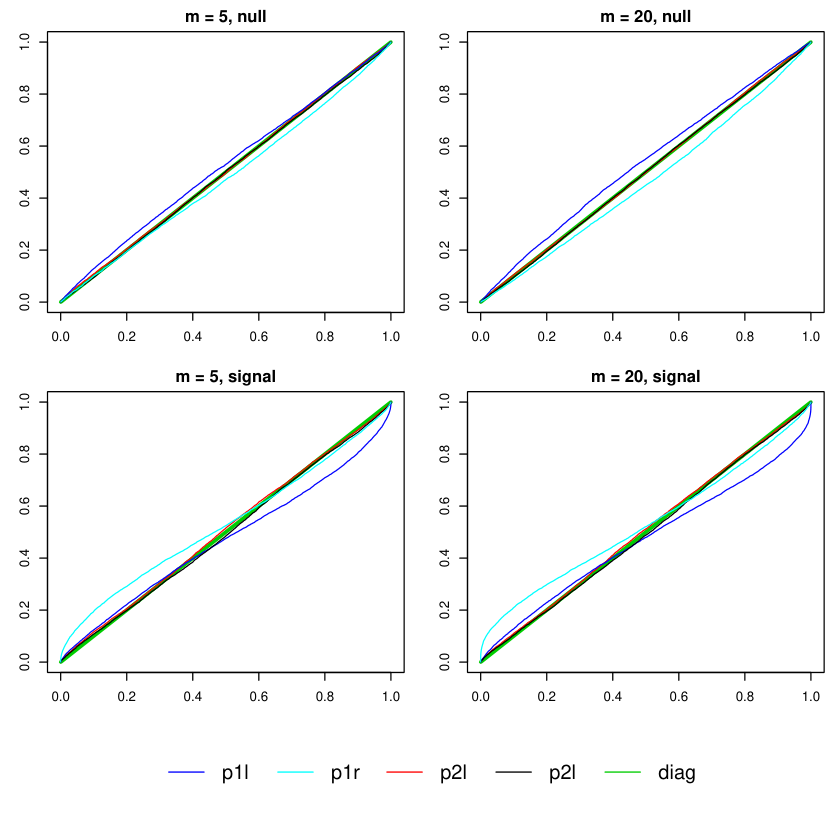
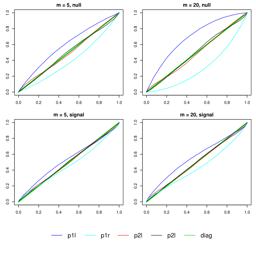
The de-biased estimate Bootstrap has p-value distribution closer to uniform – it has less dependence on the correct underlying distribution than the native Bootstrap procedure. Also, the mean rescaling approach leads to better p-value distribution.
Appendix B Proofs of Theorem 1, 2 , Lemma 1
Proposition 1.
Suppose the consistency, range, moment and dimension assumptions hold. For all , let and where is the coefficients from the model fitted with a training set of size and is the coefficient vector it converges in the consistency assumption. Let be a test set of size , then there exists a constant large enough, such that,
with and as .
Proof.
The first statement is a direct application of CLT. For the second and the third statements, we divide into and bound by two parts:
- •
By Cauchy-Schwarz inequality, we have ( and are independent). The second half by the consistency assumption. For the first term, we have
is bounded because is bounded. Now, we show that, when the range assumption holds, for a large enough constant . Imagine now we have another training data set , with sample size , and let be the coefficient trained using this dataset. By the KKT condition, we have , hence, the following is true
We know that can be arbitrarily large and grow to faster than . By LLN, for any fixed , we let and converges to a finite constant in probability. By the consistency assumption, we have . By the range assumption, for a large enough constant , we have
Hence, we have .
- •
By LLN, the moment assumption and consistency assumption, we have .
- •
By Cauchy-Schwarz inequality and LLN again, we see that the second terms in both expressions go to 0:
Hence, we have . ∎
The above results also hold if we exclude predictor . Let and for . Let and be their mean over samples for . Let be the mean of . As a direct result of Proposition 1, let be the mean validation error at penalty and fold , for a constant large enough, we have
| (7) |
Proof of Lemma 1: Let . We divide the covariance estimate into three parts:
- •
The term by LLN.
- •
As a result, we have . Now we show that that for a large constant . Let be the coefficient trained for predicting fold , we have
Bothe the first term and the second terms are bounded by equation (7). We thus prove that is bounded.
Proof of Lemma 2: Let be the coefficients trained for fold at penalty . By definition . Because both and are finite, we only need to show that for each and , we have . Let for be new realizations, we know that
Let . By Proposition 1 , we know that . By the Cauchy-Schwarz inequality, , and equivalently, . Following exactly the same argument, we have .
Proof of Theorem 1
Proposition 2.
(Guan (2018)) Let m be a fixed number and , be m dimensional vectors such that and , and is asymptotically bounded. For a sequence of bounded function that is almost everywhere differentiable with bounded first derivative under both the measures of and asymptotically, we have
We apply Proposition 1 to the cross-validation error curve, we have , where and is bounded but potentially not invertible. By Proposition 1, we know . As a consequence, and are asymptotically independent with invertible covariance matrix when :
Let and be the normal vectors from the limiting distribution corresponding to and . The asymptotic independence guarantees that any selection using has diminishing effect in :
In our case the vector and are both square integrable by equation (7) in Proposition 1 and Lemma 1:
Because has invertible covariance matrix and for each , it is almost everywhere differentiable with first derivative being 0 under both the measures of and . Based on Proposition 2, and the independence between and , we have
Finally, we apply Lemma 2, we have . Similarly, we have .
Appendix C A post selection inference approach conditional on the selected penalty
While the Bootstrap p-value described in Section 2 tests for a quantity marginalizing out all randomness, the post selection inference approach conditional on the selected penalty . It corresponds to the case where in practice, we will fix the penalty selected from now on. The testing problem is then
In Markovic et al. (2017), let be the selected penalty, the author have conditioned on (1)the feature set is selected with penalty and all predictors. (2) is the penalty which minimizes the randomized CV curve, defined as
where with being a constant. For all , the author then compare the performance between models fitted using OLS with feature set and , trained with all data. In this section, we modify their procedure in the following three aspects: (1)For the model excluding the predictor , we train it with all predictors except for instead of restricting ourselves to . (2)We do not run OLS with all data because we only care about the out of sample performance for models produced. (3)We neglect the selection event that because we want to show that the conditional on the first event only will lead to loss of power.
We look at the test statistics , where . Let . The event can be characterized by , where is the matrix with a 1 and at entry and for , and at other entries. Let the be the covariance structure of the vector . We use for and for , etc.
Let where . The intuition is that if the three variables , and are jointly asymptotically normal, then is asymptotically independent of . We can then condition on and write the constraints in terms of ’s asymptotic behavior and achieve an asymptotic guarantee for the type error control.
Proposition 3.
(Markovic et al. (2017), Theorem 1)Let be the test statistics. If the following two assumptions hold
(1)The selection event can be characterized in terms of affine constraints over some data vector .
(2) The asymptotic joint normality of with invertible covariance matrix holds pre-selection
Let , be the normal vectors from the limiting distribution, then we have
The proposition also works for the one side test. By Proposition 1, we know and are asymptotically jointly normal with invertible covariance matrix. Hence, we can construct the p-value for any hypothesis value we are interested in based on Lemma 3:
Lemma 3.
Let be the hypothesized mean of and be the normal variable from the limiting distribution of . Under the consistency, moment and dimension assumptions, we have
- 1.
The following construction of p-value achieving the asymptotic uniformity under the simple null hypothesis parameter ,
with , .
- 2.
The type I error for the null can be controlled by controlling type I error at : .
By convention, we let represent the element of vector , the maximum of an empty set is and the minimum of an empty set is .
Proposition 4.
(Lee et al. (2016), Lemma A.1)Let denote the cumulative distribution function of a Gaussian random variable with mean and variance whose domain of is . is monotone decreasing in .
References
- Berk et al. (2013) Berk, R., Brown, L., Buja, A., Zhang, K., Zhao, L. et al. (2013), ‘Valid post-selection inference’, The Annals of Statistics 41(2), 802–837.
- Breiman (2001) Breiman, L. (2001), ‘Random forests’, Machine learning 45(1), 5–32.
- Eberlin et al. (2014) Eberlin, L. S., Tibshirani, R. J., Zhang, J., Longacre, T. A., Berry, G. J., Bingham, D. B., Norton, J. A., Zare, R. N. & Poultsides, G. A. (2014), ‘Molecular assessment of surgical-resection margins of gastric cancer by mass-spectrometric imaging’, Proceedings of the National Academy of Sciences 111(7), 2436–2441.
- Fithian et al. (2014) Fithian, W., Sun, D. & Taylor, J. (2014), ‘Optimal inference after model selection’, arXiv preprint arXiv:1410.2597 .
- Friedman et al. (2001) Friedman, J., Hastie, T. & Tibshirani, R. (2001), The elements of statistical learning, Vol. 1, Springer series in statistics New York.
- Guan (2018) Guan, L. (2018), ‘Test error estimation after model selection using validation error’, arXiv preprint arXiv:1801.02817 .
- Harris (2016) Harris, X. T. (2016), ‘Prediction error after model search’, arXiv preprint arXiv:1610.06107 .
- Lee et al. (2016) Lee, J. D., Sun, D. L., Sun, Y., Taylor, J. E. et al. (2016), ‘Exact post-selection inference, with application to the lasso’, The Annals of Statistics 44(3), 907–927.
- Lee & Taylor (2014) Lee, J. D. & Taylor, J. E. (2014), Exact post model selection inference for marginal screening, in ‘Advances in Neural Information Processing Systems’, pp. 136–144.
- Lei (2017) Lei, J. (2017), ‘Cross-validation with confidence’, arXiv preprint arXiv:1703.07904 .
- Markovic et al. (2017) Markovic, J., Xia, L. & Taylor, J. (2017), ‘Adaptive p-values after cross-validation’, arXiv preprint arXiv:1703.06559 .
- Meinshausen & Bühlmann (2010) Meinshausen, N. & Bühlmann, P. (2010), ‘Stability selection’, Journal of the Royal Statistical Society: Series B (Statistical Methodology) 72(4), 417–473.
- Rhee et al. (2003) Rhee, S.-Y., Gonzales, M. J., Kantor, R., Betts, B. J., Ravela, J. & Shafer, R. W. (2003), ‘Human immunodeficiency virus reverse transcriptase and protease sequence database’, Nucleic acids research 31(1), 298–303.
- Rinaldo et al. (2016) Rinaldo, A., Wasserman, L., G’Sell, M., Lei, J. & Tibshirani, R. (2016), ‘Bootstrapping and sample splitting for high-dimensional, assumption-free inference’, arXiv preprint arXiv:1611.05401 .
- Tibshirani et al. (2015) Tibshirani, R. J., Rinaldo, A., Tibshirani, R. & Wasserman, L. (2015), ‘Uniform asymptotic inference and the bootstrap after model selection’, arXiv preprint arXiv:1506.06266 .
- Tibshirani et al. (2016) Tibshirani, R. J., Taylor, J., Lockhart, R. & Tibshirani, R. (2016), ‘Exact post-selection inference for sequential regression procedures’, Journal of the American Statistical Association 111(514), 600–620.
- Tibshirani & Tibshirani (2009) Tibshirani, R. J. & Tibshirani, R. (2009), ‘A bias correction for the minimum error rate in cross-validation’, The Annals of Applied Statistics pp. 822–829.
- Wainwright (2009) Wainwright, M. J. (2009), ‘Sharp thresholds for high-dimensional and noisy sparsity recovery using _ 1-constrained quadratic programming (lasso)’, IEEE transactions on information theory 55(5), 2183–2202.
- Yu et al. (2018) Yu, Y., Bradic, J. & Samworth, R. J. (2018), ‘Confidence intervals for high-dimensional cox models’, arXiv preprint arXiv:1803.01150 .
- Zhang & Zhang (2014) Zhang, C.-H. & Zhang, S. S. (2014), ‘Confidence intervals for low dimensional parameters in high dimensional linear models’, Journal of the Royal Statistical Society: Series B (Statistical Methodology) 76(1), 217–242.
- Zhu & Bradic (2017) Zhu, Y. & Bradic, J. (2017), ‘Breaking the curse of dimensionality in regression’, arXiv preprint arXiv:1708.00430 .