跳到论文正文
W Papers独立论文阅读器 arXiv:1806.01187 论文正文 计算阅读时间 · 0%
引用这篇论文根据当前论文元数据生成,正式投稿前建议核对。


License: arXiv.org perpetual non-exclusive license
arXiv:1806.01187v2 [math.NT] 07 Mar 2019

Maass forms and the mock theta function f⁡(q)f(q)Thanks: The first author was supported by a grant from the Simons Foundation (#426145 to Scott Ahlgren).

Scott Ahlgren Address: Department of Mathematics
University of Illinois
Urbana, IL 61801
Email address: sahlgren@illinois.edu
and Alexander Dunn Address: Department of Mathematics
University of Illinois
Urbana, IL 61801
Email address: ajdunn2@illinois.edu Dedicated to George Andrews on the occasion of his 80th birthday. Dedicated to George Andrews on the occasion of his 80th birthday.
Date: August 24, 2026
Abstract.

Let f⁡(q):=1+∑n=1∞α⁡(n)​qnf(q):=1+\sum_{n=1}^{\infty}\alpha(n)q^{n} be the well-known third order mock theta of Ramanujan. In 1964, George Andrews proved an asymptotic formula of the form

α⁡(n)=∑c≤nψ⁡(n)+Oϵ​(nϵ),\alpha(n)=\sum_{c\leq\sqrt{n}}\psi(n)+O_{\epsilon}\left(n^{\epsilon}\right),

where ψ⁡(n)\psi(n) is an expression involving generalized Kloosterman sums and the II-Bessel function. Andrews conjectured that the series converges to α⁡(n)\alpha(n) when extended to infinity, and that it does not converge absolutely. Bringmann and Ono proved the first of these conjectures. Here we obtain a power savings bound for the error in Andrews’ formula, and we also prove the second of these conjectures.

Our methods depend on the spectral theory of Maass forms of half-integral weight, and in particular on an average estimate for the Fourier coefficients of such forms which gives a power savings in the spectral parameter.

As a further application of this result, we derive a formula which expresses α⁡(n)\alpha(n) with small error as a sum of exponential terms over imaginary quadratic points (this is similar in spirit to a recent result of Masri). We also obtain a bound for the size of the error term incurred by truncating Rademacher’s analytic formula for the ordinary partition function which improves a result of the first author and Andersen when 24​n−2324n-23 is squarefree.

2010 Mathematics Subject Classification
11F30, 11F37, 11L05, 11P82

1. Introduction

Let

(1.1) f⁡(q):=1+∑n=1∞α⁡(n)​qn=1+∑n=1∞qn2(1+q)2(1+q2)2⋯(1+qn)2f(q):=1+\sum_{n=1}^{\infty}\alpha(n)q^{n}=1+\sum_{n=1}^{\infty}\frac{q^{n^{2}}}{(1+q)^{2}(1+q^{2})^{2}\cdots(1+q^{n})^{2}}

be the famous third-order mock theta function of Ramanujan. One may consult for example [BO06], [BFOR17], [Duk14], and [Zag09] and the references therein for an account of the substantial body of research related to this and to other mock theta functions. Part of the importance of the function f⁡(q)f(q) arises from the fact that the coefficients α⁡(n)\alpha(n) are related to a fundamental combinatorial statistic. In particular, we have

α⁡(n)=Ne​(n)−No​(n),\alpha(n)=N_{\rm e}(n)-N_{\rm o}(n),

where these denote the number of partitions of even and odd rank respectively.

Ramanujan recorded an asymptotic formula for α⁡(n)\alpha(n) in his last letter to Hardy in 1920; this was proved in 1951 by Dragonette [Dra52]. Andrews [And66] made a major breakthrough in his 1964 Ph.D. thesis by proving the remarkable formula (valid for any ϵ>0\epsilon>0)

(1.2) α⁡(n)=π(24​n−1)14​∑c=1⌊n⌋(−1)⌊c+12⌋​A2​c​(n−c⁡(1+(−1)c)4)c​I12​(π​24​n−112​c)+Oϵ​(nϵ).\alpha(n)=\frac{\pi}{(24n-1)^{\frac{1}{4}}}\sum_{c=1}^{\lfloor\sqrt{n}\rfloor}\frac{(-1)^{\lfloor\frac{c+1}{2}\rfloor}A_{2c}\left(n-\frac{c(1+(-1)^{c})}{4}\right)}{c}I_{\frac{1}{2}}\left(\frac{\pi\sqrt{24n-1}}{12c}\right)+O_{\epsilon}(n^{\epsilon}).

Here I12I_{\frac{1}{2}} is the II–Bessel function of order 1/21/2, and Ac​(n)A_{c}(n) is the generalized Kloosterman sum

(1.3) Ac​(n):=∑d(modc)(d,c)=1eπ​i​s​(d,c)​e​(−d​nc),c,n∈ℕ,A_{c}(n):=\sum_{\begin{subarray}{c}d\pmod{c}\\ (d,c)=1\end{subarray}}e^{\pi is(d,c)}e\left(-\frac{dn}{c}\right),\qquad c,n\in\mathbb{N},

where s⁡(d,c)s(d,c) is the Dedekind sum defined in (3.2) below and e⁡(x):=exp⁡(2​π​i​x)e(x):=\exp(2\pi ix).

Andrews [And66, p. 456], [And03, §5] conjectured that

(1.4) α⁡(n)=π(24​n−1)14​∑c=1∞(−1)⌊c+12⌋​A2​c​(n−c⁡(1+(−1)c)4)c​I12​(π​24​n−112​c),\alpha(n)=\frac{\pi}{(24n-1)^{\frac{1}{4}}}\sum_{c=1}^{\infty}\frac{(-1)^{\lfloor\frac{c+1}{2}\rfloor}A_{2c}\left(n-\frac{c(1+(-1)^{c})}{4}\right)}{c}I_{\frac{1}{2}}\left(\frac{\pi\sqrt{24n-1}}{12c}\right),

and that the series does not converge absolutely. We note that by a result of Lehmer [Leh38, Theorem 8] we have the Weil-type bound

(1.5) |A2​c​(n−c⁡(1+(−1)c)4)|≤2ωo​(c)​2​c,\left|A_{2c}\left(n-\mathord{\raise 0.49991pt\hbox{$\displaystyle\genfrac{}{}{0.4pt}{}{c(1+(-1)^c)}{4}$}}\right)\right|\leq 2^{\omega_{o}(c)}\sqrt{2c},

where ωo​(c)\omega_{o}(c) is the number of distinct odd prime divisors of cc (we give a refinement of this result in Section 9 below). This bound does not suffice to prove convergence.

The formula (1.4) was proved by Bringmann and Ono [BO06] in 2006 using the theory of harmonic Maass forms, and in particular the work of Zwegers [Zwe02] which packaged Watson’s transformation properties [Wat36] for f⁡(q)f(q) in a three dimensional vector of real-analytic modular forms.

Here we return to the question of obtaining an effective error estimate for the approximation to α⁡(n)\alpha(n) by the truncation of the series (1.2). To this end, we define the error term R⁡(n,N)R(n,N) by

(1.6) α⁡(n)=π(24​n−1)14​∑c≤N(−1)⌊c+12⌋​A2​c​(n−c⁡(1+(−1)c)4)c​I12​(π​24​n−112​c)+R⁡(n,N).\alpha(n)=\frac{\pi}{(24n-1)^{\frac{1}{4}}}\sum_{c\leq N}\frac{(-1)^{\lfloor\frac{c+1}{2}\rfloor}A_{2c}\left(n-\frac{c(1+(-1)^{c})}{4}\right)}{c}I_{\frac{1}{2}}\left(\frac{\pi\sqrt{24n-1}}{12c}\right)+R(n,N).

Then the result of Andrews gives

(1.7) R(n,n)≪ϵnϵ.R(n,\sqrt{n})\ll_{\epsilon}n^{\epsilon}.

Our first main result gives a power-saving improvement.

Theorem 1.1.

Suppose that 24​n−124n-1 is positive and squarefree. Then for all ϵ>0\epsilon>0 and γ>0\gamma>0 we have

R(n,γn)≪γ,ϵn−1147+ϵ.R(n,\gamma\sqrt{n})\ll_{\gamma,\epsilon}n^{-\frac{1}{147}+\epsilon}.

As a corollary, we see that when nn is sufficiently large, α⁡(n)\alpha(n) is the closest integer to the truncated sum appearing in (1.2). It would be interesting to quantify what “sufficiently large” means here.

It is also interesting to note that if one assumes the Ramanujan–Lindelöf conjecture for the coefficients of Maass cusp forms of weight 1/21/2 the present methods would yield

R(n,γn)≪γ,ϵn−116+ϵ,R(n,\gamma\sqrt{n})\ll_{\gamma,\epsilon}n^{-\frac{1}{16}+\epsilon},

while the analogue of the Linnik–Selberg conjecture for the sums of generalized Kloosterman sums which arise in the proof would give

R(n,γn)≪γ,ϵn−14+ϵ.R(n,\gamma\sqrt{n})\ll_{\gamma,\epsilon}n^{-\frac{1}{4}+\epsilon}.

We prove the second conjecture of Andrews mentioned above using a character sum identity proved in Section 9 together with an equidistribution result of Duke, Friedlander and Iwaniec [DFI95] for solutions of quadratic congruences to prime moduli.

Theorem 1.2.

The series (1.4) does not converge absolutely for any value of nn.

For squarefree values of 24​n−124n-1, Masri [Mas16, Theorem 1.3] obtained an asymptotic formula of the form

α⁡(n)=M⁡(n)+Oϵ​(n−1240+ϵ),\alpha(n)=M(n)+O_{\epsilon}\left(n^{-\frac{1}{240}+\epsilon}\right),

where M⁡(n)M(n) is a twisted finite sum of terms exp⁡(2​π​Im⁡τ)\exp(2\pi\im\tau) as τ\tau ranges over distinguished Galois orbits of Heegner points on X0​(6)X_{0}(6). This relies on a general power saving bound for traces of modular functions over such orbits, as well as a result of Alfes [Alf14] which relates the values α⁡(n)\alpha(n) to traces of certain real-analytic modular functions.

As a consequence of Theorem 1.1 and the results in Section 9, we obtain an asymptotic formula for α⁡(n)\alpha(n) as a sum over a set of quadratic points in the upper half-plane ℍ\mathbb{H}. Suppose that D>0D>0, and define

𝒬−D,12:={ax2+bxy+cy2:b2−4ac=−D, 12∣a,a>0}.\mathcal{Q}_{-D,12}:=\left\{ax^{2}+bxy+cy^{2}:b^{2}-4ac=-D,\ 12\mid a,\ a>0\right\}.

Then Γ0​(12)\Gamma_{0}(12) acts on this set from the left and preserves b(mod12)b\pmod{12}. If Q=[12​a,b,c]∈𝒬−D,12Q=[12a,b,c]\in\mathcal{Q}_{-D,12}, define χ−12​(Q)=(−12b)\chi_{-12}(Q)=\left(\frac{-12}{b}\right), and let τQ\tau_{Q} denote the root of Q⁡(τ,1)Q(\tau,1) in ℍ\mathbb{H}, so that g​τQ=τg​Qg\tau_{Q}=\tau_{gQ} for g∈Γ0​(12)g\in\Gamma_{0}(12). From this discussion the summands in the next theorem are well-defined.

Theorem 1.3.

Suppose that 24​n−124n-1 is positive and squarefree. Then for all ϵ>0\epsilon>0 and γ>0\gamma>0 we have

α⁡(n)=i24​n−1​∑Q∈Γ∞\𝒬1−24​n,12Im⁡τQ>γχ−12​(Q)​(e⁡(τQ)−e⁡(τ¯Q))+Oγ,ϵ​(n−1147+ϵ).\alpha(n)=\frac{i}{\sqrt{24n-1}}\sum_{\begin{subarray}{c}Q\in\Gamma_{\infty}\backslash\mathcal{Q}_{1-24n,12}\\ \im\tau_{Q}>\gamma\end{subarray}}\chi_{-12}(Q)\left(e(\tau_{Q})-e(\overline{\tau}_{Q})\right)+O_{\gamma,\epsilon}\left(n^{-\frac{1}{147}+\epsilon}\right).

Our methods depend on bounds for sums of Kloosterman sums attached to a half-integral weight multiplier on Γ0​(2)\Gamma_{0}(2) which are uniform with respect to all parameters. These depend in turn on the spectral theory of Maass forms, and in particular on average bounds for the coefficients ρ⁡(n)\rho(n) of such forms which are uniform both in the argument nn and with respect to the Laplace eigenvalue λ\lambda. We rely on three such bounds to treat various ranges of the parameters involved. The first two are recent results of Andersen-Duke and of the first author with Andersen. The third is a new bound which is important in obtaining the exponent −1147-\frac{1}{147} which appears in the theorems above. This result (which holds in any level) gives a significant improvement in λ\lambda aspect at the cost of a small loss in nn aspect; it is recorded as Theorem 4.3 below.

The series (1.4) is reminiscent of Rademacher’s well-known series [Rad36, Rad43] for the ordinary partition function p⁡(n)p(n):

(1.8) p⁡(n)=2​π(24​n−1)34​∑c=1∞Ac​(n)c​I32​(π​24​n−16​c)p(n)=\frac{2\pi}{(24n-1)^{\frac{3}{4}}}\sum_{c=1}^{\infty}\frac{A_{c}(n)}{c}I_{\frac{3}{2}}\left(\frac{\pi\sqrt{24n-1}}{6c}\right)

(this does converge absolutely, in contrast with (1.4)). A classical problem is to estimate the error associated with truncating this series, and the methods of this paper give an improvement for this estimate. In analogy with (1.6), define S⁡(n,N)S(n,N) by

p⁡(n):=2​π(24​n−1)34​∑c≤NAc​(n)c​I32​(π​24​n−16​c)+S⁡(n,N).p(n):=\frac{2\pi}{(24n-1)^{\frac{3}{4}}}\sum_{c\leq N}\frac{A_{c}(n)}{c}I_{\frac{3}{2}}\left(\frac{\pi\sqrt{24n-1}}{6c}\right)+S(n,N).

Rademacher [Rad36, Rad43] proved that S(n,γn)≪γn−14S(n,\gamma\sqrt{n})\ll_{\gamma}n^{-\frac{1}{4}}, and Lehmer [Leh38] improved this to S(n,γn)≪γn−12lognS(n,\gamma\sqrt{n})\ll_{\gamma}n^{-\frac{1}{2}}\log n. When 24​n−2324n-23 is squarefree, Folsom and Masri [FM10] proved that

S⁡(n,n6)≪n−12−δfor someδ>0.S\left(n,\sqrt{\mathord{\raise 0.49991pt\hbox{$\displaystyle\genfrac{}{}{0.4pt}{}{n}{6}$}}}\right)\ll n^{-\frac{1}{2}-\delta}\quad\text{for some}\quad\delta>0.

Recently the first author and Andersen [AA18] obtained the bound

S(n,γn)≪γ,ϵn−12−1168+ϵ.S\left(n,\gamma\sqrt{n}\right)\ll_{\gamma,\epsilon}n^{-\frac{1}{2}-\frac{1}{168}+\epsilon}.

As another application of Theorem 4.3, we obtain the following.

Theorem 1.4.

Suppose that 24​n−2324n-23 is positive and squarefree. Then for all ϵ>0\epsilon>0 and γ>0\gamma>0 we have

S(n,γn)≪γ,ϵn−12−1147+ϵ.S(n,\gamma\sqrt{n})\ll_{\gamma,\epsilon}n^{-\frac{1}{2}-\frac{1}{147}+\epsilon}.

We close with a brief outline of the contents of the paper. In the next section, we develop some background material on the spectral theory of automorphic forms and Kloosterman sums. In Section 3 we develop the properties of a particular multiplier which is related to the coefficients of f⁡(q)f(q).

To prove Theorem 1.1 requires bounds for sums of Kloosterman sums which are uniform in all parameters. The analysis in Section 7 is similar to that of [AA18] (and is similar in spirit to the work of Sarnak and Tsimerman [ST09] in weight 00 on SL2​(ℤ){\rm SL}_{2}(\mathbb{Z}), although significant complications arise from the multiplier of weight 12\frac{1}{2}). The Kuznetsov trace formula is the basic tool to relate sums of Kloosterman sums to the coefficients of Maass forms. Section 6 contains a version of the Kuznetsov formula in the mixed sign case for half integral weight multipliers, Section 7 contains the analysis which proves Theorem 1.1, and Section 8 contains a sketch of the proof of Theorem 1.4.

In Section 4 we state three estimates for coefficients of Maass forms which are crucial for our work. The first is a mean value estimate which was recently proved by Andersen and Duke [AD18]. The second, which was proved in [AA18], is an average version of a well-known result of Duke [Duk88].

The third is the average estimate Theorem 4.3 mentioned above; the proof of this result is quite involved, and occupies Section 5. We make crucial use of a version of the Kuznetsov trace formula which appears in a recent paper of Duke, Friedlander and Iwaniec [DFI12]. We follow the basic method of Duke [Duk88] but with a modified test function which leads to a savings with respect to the spectral parameter. Duke’s method relies in turn on estimates of Iwaniec [Iwa87] for averages of Kloosterman sums in level aspect. One of the terms arising from the Kusnetsov formula is an infinite sum over weights ℓ\ell of spaces of holomorphic cusp forms, and much of the technical difficulty arises from the need to bound the summands uniformly in terms of ℓ\ell.

In Section 9 we prove the key identity Proposition 9.1 which expresses the Kloosterman sums arising in (1.2) as Weyl-type sums, and we use this identity to prove Theorem 1.3. Finally, in the last section we prove Theorem 1.2.

In the body of the paper we make the following convention: in equations which involve an arbitrary small positive quantity ϵ\epsilon, the constants which are implied by the notation ≪\ll or OO are allowed to depend on ϵ\epsilon. Any other dependencies in the implied constants will be explicitly noted.

Acknowledgments

We thank Nick Andersen and Wadim Zudilin for their helpful comments. We also thank the referee for comments which improved our exposition.

2. Background

We begin with some brief background material on Maass forms with general weight and multiplier. For more details one may consult [AA18, Section 2], [DFI12, Section 2] (where it is assumed that the cusp ∞\infty is singular), or [Sar84].

Let kk be a real number and let ℍ\mathbb{H} denote the upper half-plane. For γ=(abcd)∈SL2​(ℝ)\gamma=\left(\begin{matrix}a&b\\ c&d\end{matrix}\right)\in{\rm SL}_{2}(\mathbb{R}) and τ=x+i​y∈ℍ\tau=x+iy\in\mathbb{H}, we define

j⁡(γ,τ):=c​τ+d|c​τ+d|=ei​arg⁡(c​τ+d)j(\gamma,\tau):=\frac{c\tau+d}{|c\tau+d|}=e^{i\arg(c\tau+d)}

and the weight kk slash operator by

f|k​γ:=j​(γ,τ)−k​f​(γ​τ),f\big|_{k}\gamma:=j(\gamma,\tau)^{-k}f(\gamma\tau),

where we choose the argument in (−π,π](-\pi,\pi].

For each kk, the Laplacian

(2.1) Δk:=y2​(∂2∂x2+∂2∂y2)−i​k​y​∂∂x\Delta_{k}:=y^{2}\bigg(\frac{\partial^{2}}{\partial x^{2}}+\frac{\partial^{2}}{\partial y^{2}}\bigg)-iky\frac{\partial}{\partial x}

commutes with the weight kk slash operator.

For simplicity we will work only with the groups Γ0​(N)\Gamma_{0}(N) for N∈ℕN\in\mathbb{N} and with weights k∈12​ℤk\in\frac{1}{2}\mathbb{Z}, although much of what is said here holds in more generality. Let Γ\Gamma denote such a group. We say that ν:Γ→ℂ×\nu:\Gamma\rightarrow\mathbb{C}^{\times} is a multiplier system of weight kk if

  • •

    |ν|=1|\nu|=1

  • •

    ν⁡(−I)=e−π​i​k\nu(-I)=e^{-\pi ik}, and

  • •

    ν⁡(γ1​γ2)​j​(γ1​γ2,τ)k=ν⁡(γ1)​ν​(γ2)​j​(γ2,τ)k​j​(γ1,γ2​τ)k\nu(\gamma_{1}\gamma_{2})j(\gamma_{1}\gamma_{2},\tau)^{k}=\nu(\gamma_{1})\nu(\gamma_{2})j(\gamma_{2},\tau)^{k}j(\gamma_{1},\gamma_{2}\tau)^{k} for all γ1,γ2∈Γ\gamma_{1},\gamma_{2}\in\Gamma.

Given a cusp 𝔞\mathfrak{a}, let Γ𝔞:={γ∈Γ:γ​𝔞=𝔞}\Gamma_{\mathfrak{a}}:=\{\gamma\in\Gamma:\gamma\mathfrak{a}=\mathfrak{a}\} denote the stabilizer in Γ\Gamma and let σ𝔞\sigma_{\mathfrak{a}} denote the unique (up to translation on the right) matrix in SL2​(ℝ){\rm SL}_{2}(\mathbb{R}) satisfying σ𝔞​∞=𝔞\sigma_{\mathfrak{a}}\infty=\mathfrak{a} and σ𝔞−1​Γ𝔞​σ𝔞=Γ∞\sigma_{\mathfrak{a}}^{-1}\Gamma_{\mathfrak{a}}\sigma_{\mathfrak{a}}=\Gamma_{\infty}. Define αν,𝔞∈[0,1)\alpha_{\nu,\mathfrak{a}}\in[0,1) by the condition

ν⁡(σ𝔞​(1101)​σ𝔞−1)=e⁡(−αν,𝔞).\nu\left(\sigma_{\mathfrak{a}}\left(\begin{matrix}1&1\\ 0&1\end{matrix}\right)\sigma_{\mathfrak{a}}^{-1}\right)=e\left({-\alpha_{\nu,\mathfrak{a}}}\right).

The cusp 𝔞\mathfrak{a} is singular with respect to ν\nu if αν,𝔞=0\alpha_{\nu,\mathfrak{a}}=0. When 𝔞=∞\mathfrak{a}=\infty we suppress the subscript.

If ν\nu is multiplier of weight kk, then it is a multiplier in any weight k′≡kmod2k^{\prime}\equiv k\mod 2, and ν¯\overline{\nu} is a multiplier of weight −k-k. If αν=0\alpha_{\nu}=0 then αν¯=0\alpha_{\overline{\nu}}=0, while if αν>0\alpha_{\nu}>0 then αν¯=1−αν\alpha_{\overline{\nu}}=1-\alpha_{\nu}. For n∈ℤn\in\mathbb{Z} we define

nν:=n−αν;n_{\nu}:=n-\alpha_{\nu};

then we have

(2.2) nν¯={−(1−n)νif αν≠0,nif αν=0.n_{\overline{\nu}}=\begin{cases}-(1-n)_{\nu}\quad&\text{if $\alpha_{\nu}\neq 0$},\\ n\quad&\text{if $\alpha_{\nu}=0$}.\end{cases}

With this notation we define the generalized Kloosterman sum (at the cusp ∞\infty) by

(2.3) S⁡(m,n,c,ν):=∑0≤a,d<cγ=(abcd)∈Γν¯​(γ)​e​(mν​a+nν​dc).S(m,n,c,\nu):=\sum_{\begin{subarray}{c}0\leq a,d<c\\ \gamma=\left(\begin{smallmatrix}a&b\\ c&d\end{smallmatrix}\right)\in\Gamma\end{subarray}}\overline{\nu}(\gamma)e\left(\frac{m_{\nu}a+n_{\nu}d}{c}\right).

We have the relationships

(2.4) S⁡(m,n,c,ν)¯={S⁡(1−m,1−n,c,ν¯)if αν>0,S⁡(−m,−n,c,ν¯)if αν=0.\overline{S(m,n,c,\nu)}=\begin{cases}S(1-m,1-n,c,\overline{\nu})&\quad\text{if $\alpha_{\nu}>0$,}\\ S(-m,-n,c,\overline{\nu})&\quad\text{if $\alpha_{\nu}=0$.}\end{cases}

Two important multipliers of weight 12\frac{1}{2} are the eta-multiplier νη\nu_{\eta} on SL2​(ℤ){\rm SL}_{2}(\mathbb{Z}), given by

(2.5) η⁡(γ​τ)=νη​(γ)​c​τ+d​η​(τ),γ=(abcd)∈SL2​(ℤ),\eta(\gamma\tau)=\nu_{\eta}(\gamma)\sqrt{c\tau+d}\,\eta(\tau),\qquad\gamma=\left(\begin{matrix}a&b\\ c&d\end{matrix}\right)\in{\rm SL}_{2}(\mathbb{Z}),

and the theta-multiplier νθ\nu_{\theta} on Γ0​(4)\Gamma_{0}(4), given by

(2.6) θ⁡(γ​τ)=νθ​(γ)​c​τ+d​θ​(τ),γ=(abcd)∈Γ0​(4).\theta(\gamma\tau)=\nu_{\theta}(\gamma)\sqrt{c\tau+d}\,\theta(\tau),\qquad\gamma=\left(\begin{matrix}a&b\\ c&d\end{matrix}\right)\in\Gamma_{0}(4).

Here η⁡(τ)\eta(\tau) and θ⁡(τ)\theta(\tau) are the two fundamental theta functions

η⁡(τ)\displaystyle\eta(\tau) :=q124​∏n=1∞(1−qn),\displaystyle:=q^{\frac{1}{24}}\prod_{n=1}^{\infty}(1-q^{n}),
θ⁡(τ)\displaystyle\theta(\tau) :=∑n=−∞∞qn2,\displaystyle:=\sum_{n=-\infty}^{\infty}q^{n^{2}},

where we use the standard notation

q:=e⁡(τ)=e2​π​i​τ.q:=e(\tau)=e^{2\pi i\tau}.

For νθ\nu_{\theta} we have the formula

(2.7) νθ​((abcd))=(cd)​ϵd−1,\nu_{\theta}\left(\!\left(\begin{matrix}a&b\\ c&d\end{matrix}\right)\!\right)=\left(\frac{c}{d}\right)\epsilon_{d}^{-1},

where (∙∙)\left(\tfrac{\bullet}{\bullet}\right) is the extended Kronecker symbol and

ϵd={1 if ​d≡1(mod4),i if ​d≡3(mod4).\epsilon_{d}=\begin{cases}1&\text{ if }d\equiv 1\pmod{4},\\ i&\text{ if }d\equiv 3\pmod{4}.\end{cases}

From this we obtain

(2.8) νθ¯​(γ)=(−1d)​νθ​(γ),γ=(abcd)∈Γ0​(4).\overline{\nu_{\theta}}(\gamma)=\left(\mathord{\raise 0.49991pt\hbox{$\displaystyle\genfrac{}{}{0.4pt}{}{-1}{d}$}}\right)\nu_{\theta}(\gamma),\qquad\gamma=\left(\begin{matrix}a&b\\ c&d\end{matrix}\right)\in\Gamma_{0}(4).

With d​μ:=d​x​d​yy2d\mu:=\frac{dx\,dy}{y^{2}}, define

∥f∥2=∫Γ0​(N)\ℍ|f|2​𝑑μ.\lVert f\rVert^{2}=\int_{\Gamma_{0}(N)\backslash\mathbb{H}}|f|^{2}\,d\mu.

Denote by ℒk​(N,ν)\mathcal{L}_{k}(N,\nu) the space of L2L^{2} functions which satisfy

(2.9) f⁡(γ​τ)=j​(γ,τ)k​ν​(γ)​f​(τ)for all γ∈Γ0​(N).f(\gamma\tau)=j(\gamma,\tau)^{k}\nu(\gamma)\,f(\tau)\qquad\text{for all $\gamma\in\Gamma_{0}(N)$.}

Let ℬk​(N,ν)\mathcal{B}_{k}(N,\nu) denote the subspace of ℒk​(N,ν)\mathcal{L}_{k}(N,\nu) consisting of smooth functions ff such that ff and Δk​f\Delta_{k}f are bounded on ℍ\mathbb{H}. Then Δk\Delta_{k} has a unique self-adjoint extension to ℒk​(N,ν)\mathcal{L}_{k}(N,\nu), which we also denote by Δk\Delta_{k}. For each singular cusp 𝔞\mathfrak{a} (and only at such cusps) there is an Eisenstein series E𝔞​(z,s)E_{\mathfrak{a}}(z,s). These provide the continuous spectrum, which covers [1/4,∞)[1/4,\infty).

The reminder of the spectrum is discrete and of finite multiplicity. We denote the discrete spectrum by

λ0≤λ1≤…,\lambda_{0}\leq\lambda_{1}\leq\dots,

where we have

λ0≥|k|2​(1−|k|2).\lambda_{0}\geq\frac{|k|}{2}\left(1-\frac{|k|}{2}\right).

One component of the discrete spectrum is provided by residues of the Eisenstein series E𝔞​(z,s)E_{\mathfrak{a}}(z,s) at possible simple poles ss with 12<s≤1\frac{1}{2}<s\leq 1; the corresponding eigenvalues have λ<14\lambda<\frac{1}{4}. The remainder of the discrete spectrum arises from Maass cusp forms.

Denote by ℒ~k​(N,ν)\widetilde{\mathcal{L}}_{k}(N,\nu) the subspace of ℒk​(N,ν)\mathcal{L}_{k}(N,\nu) spanned by eigenfunctions of Δk\Delta_{k}. If f∈ℒ~k​(N,ν)f\in\widetilde{\mathcal{L}}_{k}(N,\nu) has Laplace eigenvalue λ\lambda, then we write

λ=14+r2,r∈i(0,i/4]∪[0,∞),\lambda=\frac{1}{4}+r^{2},\qquad r\in i\,(0,i/4]\cup[0,\infty),

and refer to rr as the spectral parameter of ff. Denote by ℒ~k​(N,ν,r)\widetilde{\mathcal{L}}_{k}(N,\nu,r) the subspace of such functions. Let Wκ,μW_{\kappa,\mu} denote the usual WW-Whittaker function. Then each f∈ℒ~k​(N,ν,r)f\in\widetilde{\mathcal{L}}_{k}(N,\nu,r) has a Fourier expansion of the form

(2.10) f⁡(τ)=c0​(y)+∑nν≠0ρ⁡(n)​Wk​sgn⁡(nν)2,i​r​(4​π​|nν|​y)​e​(nν​x),f(\tau)=c_{0}(y)+\sum_{n_{\nu}\neq 0}\rho(n)W_{\frac{k\sgn(n_{\nu})}{2},ir}(4\pi|n_{\nu}|y)e(n_{\nu}x),

where

c0​(y)={0if αν≠0,0if αν=0 and r≥0,ρ⁡(0)​y12+i​rif αν=0 and r∈i(0,1/4],c_{0}(y)=\begin{cases}0\quad&\text{if $\alpha_{\nu}\neq 0$},\\ 0\quad&\text{if $\alpha_{\nu}=0$ and $r\geq 0$,}\\ \rho(0)y^{\frac{1}{2}+ir}&\text{if $\alpha_{\nu}=0$ and $r\in i(0,1/4]$,}\end{cases}

with coefficients ρ⁡(n)\rho(n) (see [Pro03, p. 3878] or [DFI12, p. 2509]) . Note that in the last case, we have ρ⁡(0)≠0\rho(0)\neq 0 only when ff arises as a residue.

Complex conjugation gives an isometry (of normed spaces)

ℒ~k​(N,ν,r)⟷ℒ~−k​(N,ν¯,r).\widetilde{\mathcal{L}}_{k}(N,\nu,r)\longleftrightarrow\widetilde{\mathcal{L}}_{-k}(N,\overline{\nu},r).

If f∈ℒ~k​(N,ν,r)f\in\widetilde{\mathcal{L}}_{k}(N,\nu,r), then using (2.10) with (2.2) and the fact that Wκ,μ∈ℝW_{\kappa,\mu}\in\mathbb{R} when κ∈ℝ\kappa\in\mathbb{R} and μ∈ℝ∪i​ℝ\mu\in\mathbb{R}\cup i\mathbb{R} [DLMF, (13.4.4), (13.14.3), (13.14.31)], we find that the coefficients ρc​(n)\rho_{c}(n) of fc:=f¯f_{c}:=\overline{f} satisfy

(2.11) ρc​(n)={ρ⁡(1−n)¯if αν>0 and n≠0,ρ⁡(−n)¯if αν=0.\rho_{c}(n)=\begin{cases}\overline{\rho(1-n)}&\quad\text{if $\alpha_{\nu}>0$ and $n\neq 0$,}\\ \overline{\rho(-n)}&\quad\text{if $\alpha_{\nu}=0$.}\end{cases}

The Maass lowering operator

Lk:=k2+2​i​y​∂∂τ¯=k2+i​y​(∂∂x+i​∂∂y)L_{k}:=\frac{k}{2}+2iy\frac{\partial}{\partial\overline{\tau}}=\frac{k}{2}+iy\left(\frac{\partial}{\partial x}+i\frac{\partial}{\partial y}\right)

gives a map

ℒ~k​(N,ν,r)⟶ℒ~k−2​(N,ν,r)\widetilde{\mathcal{L}}_{k}(N,\nu,r)\longrightarrow\widetilde{\mathcal{L}}_{k-2}(N,\nu,r)

and satisfies

(2.12) ∥Lk​f∥2=(r2+(k−1)24)​∥f∥2=(λ−k2​(1−k2))​∥f∥2.\lVert L_{k}f\rVert^{2}=\left(r^{2}+\mathord{\raise 0.49991pt\hbox{$\displaystyle\genfrac{}{}{0.4pt}{}{(k-1)^2}{4}$}}\right)\lVert f\rVert^{2}=\left(\lambda-\mathord{\raise 0.49991pt\hbox{$\displaystyle\genfrac{}{}{0.4pt}{}{k}{2}$}}\left(1-\mathord{\raise 0.49991pt\hbox{$\displaystyle\genfrac{}{}{0.4pt}{}{k}{2}$}}\right)\right)\lVert f\rVert^{2}.

From the last equation, we see that if f∈ℒ~k​(N,ν)f\in\widetilde{\mathcal{L}}_{k}(N,\nu) has the minimal eigenvalue |k|2​(1−|k|2)\frac{|k|}{2}\left(1-\frac{|k|}{2}\right), then f⁡(τ)f(\tau) is in the kernel of LkL_{k} if k≥0k\geq 0, and f¯​(τ)\overline{f}(\tau) is in the kernel of L−kL_{-k} if k<0k<0. Let Mk​(N,ν)M_{k}(N,\nu) denote the space of holomorphic modular forms of weight kk and multiplier ν\nu on Γ0​(N)\Gamma_{0}(N). Using (2.9), it follows that the function

F⁡(τ):={y−k2​f​(τ)if k≥0,yk2​f¯​(τ)if k<0F(\tau):=\begin{cases}y^{-\frac{k}{2}}f(\tau)\quad&\text{if $k\geq 0$},\\ y^{\frac{k}{2}}\overline{f}(\tau)\quad&\text{if $k<0$}\\ \end{cases}

lies in Mk​(N,ν)M_{k}(N,\nu) if k≥0k\geq 0 and in M−k​(N,ν¯)M_{-k}(N,\overline{\nu}) if k<0k<0. Also, F⁡(τ)F(\tau) is a cusp form if and only if f⁡(τ)f(\tau) is a Maass cusp form.

Suppose that f∈ℒ~k​(N,ν,r)f\in\widetilde{\mathcal{L}}_{k}(N,\nu,r). Then using (2.10) and [AA18, (2.16)], we have the expansion

(2.13) Lk​f​(τ)=c0(L)​(y)+∑nν≠0ρ(L)​(n)​W(k−2)​sgn⁡(nν)2,i​r​(4​π​|nν|​y)​e​(nν​x),L_{k}f(\tau)=c^{(L)}_{0}(y)+\sum_{n_{\nu}\neq 0}\rho^{(L)}(n)W_{\frac{(k-2)\sgn(n_{\nu})}{2},ir}(4\pi|n_{\nu}|y)e(n_{\nu}x),

where

(2.14) ρ(L)​(n)={−(r2+(k−1)24)​ρ​(n)if nν>0,ρ⁡(n)if nν<0,\rho^{(L)}(n)=\begin{cases}-\left(r^{2}+\mathord{\raise 0.49991pt\hbox{$\displaystyle\genfrac{}{}{0.4pt}{}{(k-1)^2}{4}$}}\right)\rho(n)&\quad\text{if $n_{\nu}>0$,}\\ \rho(n)&\quad\text{if $n_{\nu}<0$,}\end{cases}

and

c0(L)​(y)=(k−12−i​r)​c0​(y).c^{(L)}_{0}(y)=\left(\mathord{\raise 0.49991pt\hbox{$\displaystyle\genfrac{}{}{0.4pt}{}{k-1}{2}$}}-ir\right)c_{0}(y).

3. A multiplier on Γ0​(2)\Gamma_{0}(2) and a formula for the coefficients of f⁡(q)f(q)

Here we relate the coefficients α⁡(n)\alpha(n) to Kloosterman sums attached to a multiplier ψ\psi on Γ0​(2)\Gamma_{0}(2). For the eta-multiplier defined in the last section, we have a formula of Rademacher [Rad73, (74.11), (74.12)] which is valid for c>0c>0:

(3.1) νη​(γ)=−i​e−π​i​s​(d,c)​e​(a+d24​c),\nu_{\eta}(\gamma)=\sqrt{-i}\,e^{-\pi is(d,c)}\,e\left(\frac{a+d}{24c}\right),

where s⁡(d,c)s(d,c) is the Dedekind sum

(3.2) s⁡(d,c)=∑r=1c−1rc​(d​rc−⌊d​rc⌋−12).s(d,c)=\sum_{r=1}^{c-1}\mathord{\raise 0.49991pt\hbox{$\displaystyle\genfrac{}{}{0.4pt}{}{r}{c}$}}\,\left(\mathord{\raise 0.49991pt\hbox{$\displaystyle\genfrac{}{}{0.4pt}{}{dr}{c}$}}-\left\lfloor\!\mathord{\raise 0.49991pt\hbox{$\displaystyle\genfrac{}{}{0.4pt}{}{dr}{c}$}}\!\right\rfloor-\mathord{\raise 0.49991pt\hbox{$\displaystyle\genfrac{}{}{0.4pt}{}{1}{2}$}}\right).

For c>0c>0 and γ=(abcd)\gamma=\left(\begin{smallmatrix}a&b\\ c&d\end{smallmatrix}\right) we have another convenient formula [Kno70, §4.1]

(3.3) νη​(γ)={(dc)​e​(124​[(a+d)​c−b​d​(c2−1)−3​c]) if c is odd,(cd)​e​(124​[(a+d)​c−b​d​(c2−1)+3​d−3−3​c​d]) if c is even.\nu_{\eta}(\gamma)=\begin{cases}\left(\mathord{\raise 0.49991pt\hbox{$\displaystyle\genfrac{}{}{0.4pt}{}{d}{c}$}}\right)\,e\left(\mathord{\raise 0.49991pt\hbox{$\displaystyle\genfrac{}{}{0.4pt}{}{1}{24}$}}\left[(a+d)c-bd(c^{2}-1)-3c\right]\right)&\text{ if $c$ is odd},\\ \left(\mathord{\raise 0.49991pt\hbox{$\displaystyle\genfrac{}{}{0.4pt}{}{c}{d}$}}\right)\,e\left(\mathord{\raise 0.49991pt\hbox{$\displaystyle\genfrac{}{}{0.4pt}{}{1}{24}$}}\left[(a+d)c-bd(c^{2}-1)+3d-3-3cd\right]\right)&\text{ if $c$ is even.}\end{cases}

We have νη​(±(1b01))=e⁡(b24)\nu_{\eta}\left(\pm\left(\begin{smallmatrix}1&b\\ 0&1\end{smallmatrix}\right)\right)=e\left(\frac{b}{24}\right). Finally, if c>0c>0 we have νη​(−γ)=i​νη​(γ)\nu_{\eta}(-\gamma)=i\nu_{\eta}(\gamma) (this follows since γ\gamma and −γ-\gamma act the same way on ℍ\mathbb{H}).

For γ=(abcd)∈Γ0​(2)\gamma=\left(\begin{matrix}a&b\\ c&d\end{matrix}\right)\in\Gamma_{0}(2) define

(3.4) ψ⁡(γ)={ic/2​(−1d)​νη¯​(γ)ifc≡0(mod4),ic/2​νη¯​(γ)ifc≡2(mod4).\psi\left(\gamma\right)=\begin{cases}i^{c/2}\left(\frac{-1}{d}\right)\overline{\nu_{\eta}}(\gamma)&\text{if}\quad c\equiv 0\pmod{4},\\ i^{c/2}\overline{\nu_{\eta}}(\gamma)&\text{if}\quad c\equiv 2\pmod{4}.\end{cases}

One can compute using (3.1) to see that the real-analytic form M~\widetilde{M} appearing on page 251 of [BO06] satisfies

M~​(γ​τ)=ψ⁡(γ)​(c​τ+d)12​M~​(τ)for all γ=(abcd)∈Γ0​(2).\widetilde{M}(\gamma\tau)=\psi(\gamma)(c\tau+d)^{\frac{1}{2}}\widetilde{M}(\tau)\qquad\text{for all $\gamma=\left(\begin{matrix}a&b\\ c&d\end{matrix}\right)\in\Gamma_{0}(2)$.}

(this can also be derived from [And66, Theorem 2.2]). By [Hej83, Proposition 2.1] it follows that ψ\psi is a multiplier of weight 12\frac{1}{2} on Γ0​(2)\Gamma_{0}(2).

For the cusp ∞\infty, we have ψ⁡((1101))=e⁡(−124),\psi\left(\left(\begin{smallmatrix}1&1\\ 0&1\end{smallmatrix}\right)\right)=e\left({-\frac{1}{24}}\right), so that αψ=124\alpha_{\psi}=\frac{1}{24}. For the cusp 00 we may take σ0=(0−1/220)\sigma_{0}=\left(\begin{smallmatrix}0&-1/\sqrt{2}\\ \sqrt{2}&0\end{smallmatrix}\right). Then the formulas above give

ψ⁡(σ0​(1101)​σ0−1)=ψ⁡((10−21))=e⁡(−13).\psi\left(\sigma_{0}\left(\begin{matrix}1&1\\ 0&1\end{matrix}\right)\sigma_{0}^{-1}\right)=\psi\left(\left(\begin{matrix}1&0\\ -2&1\end{matrix}\right)\right)=e\left(-\mathord{\raise 0.49991pt\hbox{$\displaystyle\genfrac{}{}{0.4pt}{}{1}{3}$}}\right).
Lemma 3.1.

Let Ac​(n)A_{c}(n) and ψ\psi be defined as in (1.3), (3.4). Then for c>0c>0 we have

(−1)⌊c+12⌋​A2​c​(n−c⁡(1+(−1)c)4)=e⁡(18)​S⁡(0,n,2​c,ψ)¯.(-1)^{\lfloor\frac{c+1}{2}\rfloor}A_{2c}\left(n-\frac{c(1+(-1)^{c})}{4}\right)=e\left(\mathord{\raise 0.49991pt\hbox{$\displaystyle\genfrac{}{}{0.4pt}{}{1}{8}$}}\right)\overline{S(0,n,2c,\psi)}.
Proof.

This follows from a case-by-case computation using (3.1) together with the fact that s⁡(−d,c)=−s⁡(d,c)s(-d,c)=-s(d,c). ∎

Since α⁡(n)∈ℤ\alpha(n)\in\mathbb{Z}, the formula (1.4) becomes

(3.5) α⁡(n)=2​π(24​n−1)14​e​(−18)​∑c>0c≡0(mod2)S⁡(0,n,c,ψ)c​I12​(π​24​n−16​c).\alpha(n)=\frac{2\pi}{(24n-1)^{\frac{1}{4}}}e\left(-\mathord{\raise 0.49991pt\hbox{$\displaystyle\genfrac{}{}{0.4pt}{}{1}{8}$}}\right)\!\!\!\!\sum_{\begin{subarray}{c}c>0\\ c\equiv 0\pmod{2}\end{subarray}}\frac{S(0,n,c,\psi)}{c}I_{\frac{1}{2}}\left(\frac{\pi\sqrt{24n-1}}{6c}\right).

We will work in the space ℒ~12​(2,ψ)\widetilde{\mathcal{L}}_{\frac{1}{2}}(2,\psi). By the discussion above, neither cusp is singular, so there are no Eisenstein series for this multiplier.

Lemma 3.2.

For each rr, the map τ↦24​τ\tau\mapsto 24\tau gives an injection

ℒ~12​(2,ψ,r)⟶ℒ~12​(144,(12∙)​νθ,r).\widetilde{\mathcal{L}}_{\frac{1}{2}}(2,\psi,r)\longrightarrow\widetilde{\mathcal{L}}_{\frac{1}{2}}\left(144,\left(\mathord{\raise 0.49991pt\hbox{$\displaystyle\genfrac{}{}{0.4pt}{}{12}{\bullet}$}}\right)\nu_{\theta},r\right).
Proof.

It is enough to check the transformation law. Given f∈ℒ~12​(2,ψ,r)f\in\widetilde{\mathcal{L}}_{\frac{1}{2}}(2,\psi,r), define

g⁡(τ):=f⁡(24​τ)=f|12​(24001/24).g(\tau):=f(24\tau)=f\big|_{\frac{1}{2}}\left(\begin{smallmatrix}\sqrt{24}&0\\ 0&1/\sqrt{24}\end{smallmatrix}\right).

If γ=(abcd)∈Γ0​(144)\gamma=\left(\begin{smallmatrix}a&b\\ c&d\end{smallmatrix}\right)\in\Gamma_{0}(144) with c>0c>0, then we have

g|12​γ=f|12​γ′​(24001/24),g\big|_{\frac{1}{2}}\gamma=f\big|_{\frac{1}{2}}\gamma^{\prime}\,\left(\begin{smallmatrix}\sqrt{24}&0\\ 0&1/\sqrt{24}\end{smallmatrix}\right),

where γ′=(a24​bc/24d)\gamma^{\prime}=\left(\begin{smallmatrix}a&24b\\ c/24&d\end{smallmatrix}\right). Then a case by case computation using (3.4) and (3.3) shows that

ψ⁡(γ′)=(12d)​νθ​(γ).\psi(\gamma^{\prime})=\left(\mathord{\raise 0.49991pt\hbox{$\displaystyle\genfrac{}{}{0.4pt}{}{12}{d}$}}\right)\nu_{\theta}(\gamma).

The identities e⁡(1−d8)=(2d)​ϵde\left(\frac{1-d}{8}\right)=\left(\frac{2}{d}\right)\epsilon_{d} and (−1d)​ϵd=ϵd−1\left(\frac{-1}{d}\right)\epsilon_{d}=\epsilon_{d}^{-1} for odd dd are useful for this computation. ∎

4. Three estimates for the coefficients of Maass forms

The proofs of our main results will depend on three different average estimates for the Fourier coefficients of Maass forms.

The first is a restatement of a recent result of Andersen and Duke [AD18, Theorem 4.1] (we state this only in the case of the cusp ∞\infty). Suppose that ν\nu is a multiplier of weight 12\frac{1}{2} for Γ0​(N)\Gamma_{0}(N) and that for nν≠0n_{\nu}\neq 0 the bound

(4.1) ∑c>0c≡0(modN)|S⁡(n,n,c,ν)|c1+β≪ν|nν|ϵ\sum_{\begin{subarray}{c}c>0\\ c\equiv 0\pmod{N}\end{subarray}}\frac{|S(n,n,c,\nu)|}{c^{1+\beta}}\ll_{\nu}|n_{\nu}|^{\epsilon}

holds for some β∈(12,1)\beta\in(\frac{1}{2},1).

The result of [AD18] is stated for positive nn in weights ±12\pm\frac{1}{2}. To derive the statement below we use (2.2), (2.4), and (2.11). Note that the assumption (4.1) differs slightly from that of [AD18] in that nνn_{\nu} appears in place of nn on the right side; an examination of the proof shows that this is sufficient. This allows us to access the case when n=0n=0 and nν<0n_{\nu}<0, which is important in our applications.

Whenever we speak of an orthonormal basis {vj​(τ)}\{v_{j}(\tau)\} for ℒ~12​(N,ν)\widetilde{\mathcal{L}}_{\frac{1}{2}}(N,\nu), we assume that each vjv_{j} is an eigenform of Δ12\Delta_{\frac{1}{2}} with eigenvalue λj\lambda_{j} and spectral parameter rj=λj−1/4r_{j}=\sqrt{\lambda_{j}-1/4}.

Proposition 4.1 (Andersen-Duke).

Suppose that ν\nu is a multiplier on Γ0​(N)\Gamma_{0}(N) of weight 12\frac{1}{2} which satisfies (4.1). Let bj​(n)b_{j}(n) denote the coefficients of an orthonormal basis {vj​(τ)}\{v_{j}(\tau)\} for ℒ~12​(N,ν)\widetilde{\mathcal{L}}_{\frac{1}{2}}(N,\nu). Then we have

|nν|∑x≤rj≤2​x|bj(n)|2e−π​rj≪ϵ,N(x2+|n|β+ϵx1−2​βlogβx)⋅{x−12if nν>0,x12if nν<0.|n_{\nu}|\sum_{x\leq r_{j}\leq 2x}|b_{j}(n)|^{2}e^{-\pi r_{j}}\ll_{\epsilon,N}\left(x^{2}+|n|^{\beta+\epsilon}x^{1-2\beta}\log^{\beta}x\right)\cdot\begin{cases}x^{-\frac{1}{2}}\quad&\text{if $n_{\nu}>0$,}\\ x^{\frac{1}{2}}\quad&\text{if $n_{\nu}<0$.}\end{cases}

The second estimate is a restatement of [AA18, Proposition 8.2].

Proposition 4.2.

Let DD be an even fundamental discriminant and let NN be a positive integer with D|ND\mid N. Let bj​(n)b_{j}(n) denote the coefficients of an orthonormal basis {vj​(τ)}\{v_{j}(\tau)\} for ℒ~12​(N,(|D|∙)​νθ)\widetilde{\mathcal{L}}_{\frac{1}{2}}\left(N,\left(\frac{|D|}{\bullet}\right)\nu_{\theta}\right). Then for square-free n≠0n\neq 0 and x≥1x\geq 1 we have

|n|∑0≤rj≤x|bj​(n)|2ch⁡π​rj≪ϵ,N|n|37+ϵx5−sgn⁡n2.|n|\sum_{0\leq r_{j}\leq x}\frac{|b_{j}(n)|^{2}}{\ch\pi r_{j}}\ll_{\epsilon,N}|n|^{\frac{3}{7}+\epsilon}x^{5-\frac{\sgn n}{2}}.

This follows directly from [AA18, Proposition 8.2] for n>0n>0. If n<0n<0, then using (2.12), we see that the map

vj↦(rj2+116)−12​L12​vj¯v_{j}\mapsto\left(r_{j}^{2}+\mathord{\raise 0.49991pt\hbox{$\displaystyle\genfrac{}{}{0.4pt}{}{1}{16}$}}\right)^{-\frac{1}{2}}\overline{L_{\frac{1}{2}}v_{j}}

gives an isometry between the subspaces of ℒ~12​(N,(|D|∙)​νθ)\widetilde{\mathcal{L}}_{\frac{1}{2}}\left(N,\left(\frac{|D|}{\bullet}\right)\nu_{\theta}\right) and ℒ~32​(N,(|D|∙)​ν¯θ)\widetilde{\mathcal{L}}_{\frac{3}{2}}\left(N,\left(\frac{|D|}{\bullet}\right)\overline{\nu}_{\theta}\right) spanned by those forms with spectral parameter not equal to i/4i/4. Moreover, if we denote the coefficients of (rj2+116)−12​L12​vj¯\left(r_{j}^{2}+\frac{1}{16}\right)^{-\frac{1}{2}}\overline{L_{\frac{1}{2}}v_{j}} by aj​(n)a_{j}(n), then (2.11) and (2.14) give

aj​(−n)=(rj2+116)−12​bj​(n)¯for n<0.a_{j}(-n)=\left(r_{j}^{2}+\frac{1}{16}\right)^{-\frac{1}{2}}\,\overline{b_{j}(n)}\qquad\text{for $n<0$.}

The statement follows by applying the result of [AA18] to the forms in weight 32\frac{3}{2} and using partial summation.

Finally, we will prove an estimate which is slightly weaker in nn aspect than Proposition 4.2 but is significantly better in spectral parameter aspect.

Theorem 4.3.

Let DD be an even fundamental discriminant and let NN be a positive integer with D|ND\mid N. Let bj​(n)b_{j}(n) denote the coefficients of an orthonormal basis {vj​(τ)}\{v_{j}(\tau)\} for ℒ~12​(N,(|D|∙)​νθ)\widetilde{\mathcal{L}}_{\frac{1}{2}}\left(N,\left(\frac{|D|}{\bullet}\right)\nu_{\theta}\right). Then for square-free n≠0n\neq 0 and x≥1x\geq 1 we have

|n|∑|rj|≤x|bj​(n)|2ch⁡π​rj≪ϵ,N|n|131294+ϵx3−sgn⁡n2.|n|\sum_{|r_{j}|\leq x}\frac{|b_{j}(n)|^{2}}{\ch\pi r_{j}}\ll_{\epsilon,N}|n|^{\frac{131}{294}+\epsilon}x^{3-\frac{\sgn n}{2}}.

The proof of this result is somewhat involved, and occupies the next section. We follow the basic strategy of Duke [Duk88], which in turn relies on bounds of Iwaniec [Iwa87] for sums of Kloosterman sums averaged over the level. We use a recent version of the Kusnetsov trace formula due to Duke, Friedlander and Iwaniec [DFI12] which allows us to use test functions which lead to a significant savings with respect to the spectral parameter. The most delicate part of the subsequent analysis involves a sum over holomorphic cusp forms of arbitrarily large weight ℓ\ell weighted by JJ-Bessel transforms, and much of the difficulty arises in obtaining bounds which are uniform with respect to ℓ\ell.

4.1. Remarks

For individual coefficients, this theorem implies that

(4.2) bj(n)≪N,ϵλj34−sgn⁡n8ch(π​rj2)|n|−163588+ϵ.b_{j}(n)\ll_{N,\epsilon}\lambda_{j}^{\frac{3}{4}-\frac{\sgn n}{8}}\ch\left(\mathord{\raise 0.49991pt\hbox{$\displaystyle\genfrac{}{}{0.4pt}{}{\pi r_j}{2}$}}\right)|n|^{-\frac{163}{588}+\epsilon}.

This is slightly weaker in nn-aspect and significantly stronger in λ\lambda-aspect than the well-known result of Duke [Duk88, Theorem 5]. Baruch and Mao [BM10, Theorem 1.5] obtained a bound which is stronger in nn than Duke’s bound, but weaker in the spectral parameter. The approach of Baruch and Mao relies on subconvexity bounds for LL-functions due to Blomer, Harcos, and Michel [BHM07] and a Kohnen-Zagier type formula which relates special values of these LL-functions to the coefficients bj​(n)b_{j}(n). The subconvexity bounds were later improved by Blomer and Harcos [BH08]. Following the approach of Baruch and Mao using these improved bounds should lead to a bound for the individual coefficients in which the exponent −163588=−.277​…-\frac{163}{588}=-.277\dots above is replaced by −516=−.3125-\frac{5}{16}=-.3125, with the same power of λj\lambda_{j}. An average version of this bound in the style of Theorem 4.3 would improve the exponents in our applications.

A very strong average version is available in special cases due to work of Young [You17]. Young obtains estimates of the form

∑T≤rj≤T+1L(uj×χq,12)3≪ϵ(q(T+1))1+ϵ,\sum_{T\leq r_{j}\leq T+1}L(u_{j}\times\chi_{q},\tfrac{1}{2})^{3}\ll_{\epsilon}(q(T+1))^{1+\epsilon},

where qq is odd and square-free, χq\chi_{q} is a real character of conductor qq, and {uj}\{u_{j}\} is an orthonormal basis of weight zero Maass cusp forms in level dividing qq (note that there are ≍T\asymp T terms in the sum). Unfortunately this does not apply to our situation. Andersen and Duke [AD18] use Young’s result as an input to obtain strong bounds for sums of Kloosterman sums arising in the plus-space in level four (in which case the forms uju_{j} have level one), and obtain striking applications.

Finally, we mention that the Lindelöf hypothesis L(uj×χq,12)≪ϵ((1+|rj|)q)ϵL(u_{j}\times\chi_{q},\tfrac{1}{2})\ll_{\epsilon}((1+|r_{j}|)q)^{\epsilon} would lead to the pointwise bound

bj(n)≪N,ϵλj−sgn⁡n8ch(π​rj2)|n|−12+ϵ.b_{j}(n)\ll_{N,\epsilon}\lambda_{j}^{-\frac{\sgn n}{8}}\ch\left(\mathord{\raise 0.49991pt\hbox{$\displaystyle\genfrac{}{}{0.4pt}{}{\pi r_j}{2}$}}\right)|n|^{-\frac{1}{2}+\epsilon}.

This would of course lead to substantial improvements in the error bounds discussed in this paper, as described in the Introduction.

5. Proof of Theorem 4.3

5.1. The Kusnetsov formula

We follow the exposition of Duke, Friedlander and Iwaniec [DFI12, §2]. Assume that ν\nu is a multiplier on Γ0​(N)\Gamma_{0}(N), and that

αν=0.\alpha_{\nu}=0.

Let Φ:[0,∞)→ℝ\Phi:[0,\infty)\rightarrow\mathbb{R} be a smooth function such that

(5.1) Φ⁡(0)=Φ′​(0)=0\Phi(0)=\Phi^{\prime}(0)=0

and let JsJ_{s} denote the JJ-Bessel function. For s∈ℂs\in\mathbb{C}, define

Φ~​(s)=∫0∞Js​(u)​Φ​(u)​d​uu,\widetilde{\Phi}(s)=\int_{0}^{\infty}J_{s}(u)\Phi(u)\,\frac{du}{u},

and suppose that for some ϵ>0\epsilon>0 we have

(5.2) Φ~​(2​i​t)\displaystyle\widetilde{\Phi}(2it) ≪t−2−ϵchπtfor t≥1,\displaystyle\ll t^{-2-\epsilon}\ch\pi t\qquad\text{for $t\geq 1$},
(5.3) Φ~​(ℓ)\displaystyle\widetilde{\Phi}(\ell) ≪ℓ−2−ϵfor ℓ≥1.\displaystyle\ll\ell^{-2-\epsilon}\qquad\quad\,\ \ \ \text{for $\ell\geq 1$}.

Also define

Φ^​(t)=i⁡(Φ~​(2​i​t)​cos⁡π⁡(k2+i​t)−Φ~​(−2​i​t)​cos⁡π⁡(k2−i​t))​Dk​(t)sh⁡π​t,\widehat{\Phi}(t)=i\left(\widetilde{\Phi}(2it)\cos\pi\left(\mathord{\raise 0.49991pt\hbox{$\displaystyle\genfrac{}{}{0.4pt}{}{k}{2}$}}+it\right)-\widetilde{\Phi}(-2it)\cos\pi\left(\mathord{\raise 0.49991pt\hbox{$\displaystyle\genfrac{}{}{0.4pt}{}{k}{2}$}}-it\right)\right)\frac{D_{k}(t)}{\sh\pi t},

where

Dk​(t)=12​π2​Γ​(1+k2+i​t)​Γ​(1+k2−i​t).D_{k}(t)=\frac{1}{2\pi^{2}}\Gamma\left(\mathord{\raise 0.49991pt\hbox{$\displaystyle\genfrac{}{}{0.4pt}{}{1+k}{2}$}}+it\right)\Gamma\left(\mathord{\raise 0.49991pt\hbox{$\displaystyle\genfrac{}{}{0.4pt}{}{1+k}{2}$}}-it\right).

For m,n≥1m,n\geq 1 define

(5.4) 𝒦Φ(N)​(m,n):=∑c>0c≡0(modN)c−1​S​(m,n,c,ν)​Φ​(4​π​m​nc).\mathcal{K}^{(N)}_{\Phi}(m,n):=\sum_{\begin{subarray}{c}c>0\\ c\equiv 0\pmod{N}\end{subarray}}c^{-1}S(m,n,c,\nu)\Phi\left(\frac{4\pi\sqrt{mn}}{c}\right).

The Kusnetsov formula expresses 𝒦Φ(N)​(m,n)\mathcal{K}^{(N)}_{\Phi}(m,n) as the sum of three spectral terms. The first two of these correspond to the discrete and the continuous spectrums. Let {uj​(τ)}\{u_{j}(\tau)\} be an orthonormal basis for ℒ~k​(N,ν)\widetilde{\mathcal{L}}_{k}(N,\nu), and denote the coefficients by ρj​(n)\rho_{j}(n) and the spectral parameters by rjr_{j}. For each singular cusp 𝔞\mathfrak{a}, let ρ𝔞​(n,t)\rho_{\mathfrak{a}}(n,t) be the Fourier coefficients for the Eisenstein series attached to 𝔞\mathfrak{a}. Define

(5.5) ℒΦ^(N)​(m,n)\displaystyle\mathcal{L}^{(N)}_{\widehat{\Phi}}(m,n) :=4​π​m​n​∑j≥0ρj​(m)¯​ρj​(n)​Φ^​(rj)ch⁡π​rj,\displaystyle:=4\pi\sqrt{mn}\sum_{j\geq 0}\overline{\rho_{j}(m)}\rho_{j}(n)\frac{\widehat{\Phi}(r_{j})}{\ch\pi r_{j}},
(5.6) ℳΦ^(N)​(m,n)\displaystyle\mathcal{M}^{(N)}_{\widehat{\Phi}}(m,n) :=4​π​m​n​∑𝔞14​π​∫−∞∞ρ𝔞​(m,t)¯​ρ𝔞​(n,t)​Φ^​(t)ch⁡π​t​𝑑t.\displaystyle:=4\pi\sqrt{mn}\sum_{\mathfrak{a}}\frac{1}{4\pi}\int_{-\infty}^{\infty}\overline{\rho_{\mathfrak{a}}(m,t)}\rho_{\mathfrak{a}}(n,t)\frac{\widehat{\Phi}(t)}{\ch\pi t}dt.

The third term involves the holomorphic forms. For ℓ≡k(mod2)\ell\equiv k\pmod{2} with ℓ≥2\ell\geq 2, let Sℓ​(N,ν)S_{\ell}(N,\nu) denote the space of holomorphic cusp forms of weight ℓ\ell, level NN and multiplier ν\nu. Let ℬℓ\mathcal{B}_{\ell} denote an orthonormal basis of this space with respect to the Petersson inner product

⟨f,g⟩=∫Γ0​(N)∖ℍyℓ​f​(τ)​g⁡(τ)¯​𝑑μ.\langle f,g\rangle=\int_{\Gamma_{0}(N)\setminus\mathbb{H}}y^{\ell}f(\tau)\overline{g(\tau)}\,d\mu.

Every f∈ℬℓf\in\mathcal{B}_{\ell} has a Fourier expansion

(5.7) f⁡(τ)=∑n=1∞af​(n)​(4​π​n)ℓ−12​e​(n​τ).f(\tau)=\sum_{n=1}^{\infty}a_{f}(n)(4\pi n)^{\frac{\ell-1}{2}}e(n\tau).

The third spectral term is

𝒩Φˇ(N)​(m,n)=∑ℓ≡k(mod2)ℓ≥2Φˇ​(ℓ)​Γ​(ℓ)​∑f∈ℬℓaf​(m)¯​af​(n),\mathcal{N}^{(N)}_{\widecheck{\Phi}}(m,n)=\sum_{\begin{subarray}{c}\ell\equiv k\!\!\!\!\pmod{2}\\ \ell\geq 2\end{subarray}}\widecheck{\Phi}(\ell)\Gamma(\ell)\sum_{f\in\mathcal{B}_{\ell}}\overline{a_{f}(m)}a_{f}(n),

where

(5.8) Φˇ​(ℓ):=π−1​Φ~​(ℓ−1)​eπ​i​(ℓ−k)2.\widecheck{\Phi}(\ell):=\pi^{-1}\widetilde{\Phi}(\ell-1)e^{\frac{\pi i(\ell-k)}{2}}.

Define

γk:=e−π​i​k2.\gamma_{k}:=e^{-\frac{\pi ik}{2}}.

Duke, Friedlander, and Iwaniec [DFI12, Theorem 2.5, (2.28), (2.29)] proved the following.

Proposition 5.1 (Duke–Friedlander–Iwaniec).

Suppose that ν\nu is a multiplier of weight kk on Γ0​(N)\Gamma_{0}(N) with αν=0\alpha_{\nu}=0. Let Φ\Phi be a smooth function which satisfies (5.1), (5.2) and (5.3). Then for m,n≥1m,n\geq 1 we have

γk​𝒦Φ(N)​(m,n)=ℒΦ^(N)​(m,n)+ℳΦ^(N)​(m,n)+𝒩Φˇ(N)​(m,n).\gamma_{k}\mathcal{K}^{(N)}_{\Phi}(m,n)=\mathcal{L}^{(N)}_{\widehat{\Phi}}(m,n)+\mathcal{M}^{(N)}_{\widehat{\Phi}}(m,n)+\mathcal{N}^{(N)}_{\widecheck{\Phi}}(m,n).

5.2. Start of the proof of Theorem 4.3

We now suppose that DD is an even fundamental discriminant, that N≡0(mod8)N\equiv 0\pmod{8} is a positive integer with D|ND\mid N, and that

(5.9) (k,ν)=(12,(|D|∙)​νθ)or(k,ν)=(−12,(|D|∙)​νθ¯)=(−12,(−|D|∙)​νθ).(k,\nu)=\left(\mathord{\raise 0.49991pt\hbox{$\displaystyle\genfrac{}{}{0.4pt}{}{1}{2}$}},\left(\mathord{\raise 0.49991pt\hbox{$\displaystyle\genfrac{}{}{0.4pt}{}{|D|}{\bullet}$}}\right)\nu_{\theta}\right)\qquad\text{or}\qquad(k,\nu)=\left(-\mathord{\raise 0.49991pt\hbox{$\displaystyle\genfrac{}{}{0.4pt}{}{1}{2}$}},\left(\mathord{\raise 0.49991pt\hbox{$\displaystyle\genfrac{}{}{0.4pt}{}{|D|}{\bullet}$}}\right)\overline{\nu_{\theta}}\right)=\left(-\mathord{\raise 0.49991pt\hbox{$\displaystyle\genfrac{}{}{0.4pt}{}{1}{2}$}},\left(\mathord{\raise 0.49991pt\hbox{$\displaystyle\genfrac{}{}{0.4pt}{}{-|D|}{\bullet}$}}\right)\nu_{\theta}\right).

For such a multiplier ν\nu, we have the Weil bound [Wai17, Lemma 4]

(5.10) |S⁡(n,n,c,ν)|≤τ⁡(c)​(n,c)12​c12.\left|S(n,n,c,\nu)\right|\leq\tau(c)(n,c)^{\frac{1}{2}}c^{\frac{1}{2}}.

Suppose that μ∈{−1,0,1}\mu\in\{-1,0,1\}. For n∈ℕn\in\mathbb{N} and x≥1x\geq 1 we define

(5.11) Kμ(N)​(n,x):=∑c≤xc≡0(modN)c−12​S​(n,n,c,ν)​e​(2​μ​nc).K_{\mu}^{(N)}(n;x):=\sum_{\begin{subarray}{c}\\ c\leq x\\ c\equiv 0\pmod{N}\end{subarray}}c^{-\frac{1}{2}}S(n,n,c,\nu)e\left(\frac{2\mu n}{c}\right).

Let PP be a positive parameter (which will eventually be set to n17n^{\frac{1}{7}}), and define

(5.12) 𝒬=𝒬(n,N,P):={pN:pprime,P<p≤2P, andp∤2nN}.\mathcal{Q}=\mathcal{Q}(n,N,P):=\left\{pN:p\ \text{prime,}\ \ P<p\leq 2P,\text{ and}\ \ p\nmid 2nN\right\}.

For the theta-multiplier, Iwaniec [Iwa87, Theorem 3] obtained a bound for the sums Kμ(N)​(n,x)K_{\mu}^{(N)}(n;x) averaged over the level. This was extended to the case of twists by a quadratic character by Waibel [Wai17, §3] (this is also implicit in the work of Duke [Duk88]). Combining these results, we have

Proposition 5.2.

Suppose that N≡0(mod8)N\equiv 0\pmod{8}, that μ∈{−1,0,1}\mu\in\{-1,0,1\}, that n>0n>0 is square-free, and that 𝒬\mathcal{Q} is as in (5.12). Suppose that ν\nu is one of the characters appearing in (5.9). Then we have

(5.13) ∑Q∈𝒬|Kμ(Q)(n;x)|≪N,ϵ{xP−12+xn−12+(x+n)58(x14P38+n18x18P14)}(nx)ϵ.\sum_{Q\in\mathcal{Q}}\left|K_{\mu}^{(Q)}(n;x)\right|\ll_{N,\epsilon}\left\{xP^{-\frac{1}{2}}+xn^{-\frac{1}{2}}+(x+n)^{\frac{5}{8}}\left(x^{\frac{1}{4}}P^{\frac{3}{8}}+n^{\frac{1}{8}}x^{\frac{1}{8}}P^{\frac{1}{4}}\right)\right\}(nx)^{\epsilon}.

We choose the smooth function

(5.14) Φ⁡(u):=18​π2​u−12​J92​(u).\Phi(u):=\mathord{\raise 0.49991pt\hbox{$\displaystyle\genfrac{}{}{0.4pt}{}{1}{8}$}}\sqrt{\mathord{\raise 0.49991pt\hbox{$\displaystyle\genfrac{}{}{0.4pt}{}{\pi}{2}$}}}\,u^{-\frac{1}{2}}J_{\frac{9}{2}}(u).

At u=0u=0 we have the expansion Φ⁡(u)=u47560+⋯\Phi(u)=\frac{u^{4}}{7560}+\cdots, so (5.1) is satisfied. Using the Weber–Schafheitlin integral [DLMF, (10.22.57)] we compute

(5.15) Φ~​(2​i​t)=−i​t⁡(1+t2)(1+4​t2)​(9+4​t2)​(25+4​t2)​ch⁡π​tfort∈ℝ,\widetilde{\Phi}(2it)=-i\frac{t(1+t^{2})}{(1+4t^{2})(9+4t^{2})(25+4t^{2})}\ch\pi t\quad\text{for}\quad t\in\mathbb{R},

and

(5.16) Φ~​(ℓ)=−18​ℓ⁡(ℓ2−4)​cos⁡(π​ℓ2)(ℓ2−1)​(ℓ2−9)​(ℓ2−25)forℓ≥1.\widetilde{\Phi}(\ell)=-\frac{1}{8}\frac{\ell(\ell^{2}-4)\cos\left(\frac{\pi\ell}{2}\right)}{(\ell^{2}-1)(\ell^{2}-9)(\ell^{2}-25)}\quad\text{for}\quad\ell\geq 1.

Thus both (5.2) and (5.3) are satisfied (note that the cosine factor cancels the zeros in the denominator of (5.16)).

For k=±12k=\pm\frac{1}{2} we have

Φ^​(t)=2​t​(1+t2)(1+4​t2)​(9+4​t2)​(25+4​t2)​(ch⁡π​t)2​Dk​(t)sh⁡(π​t).\hat{\Phi}(t)=\frac{\sqrt{2}\,t(1+t^{2})}{(1+4t^{2})(9+4t^{2})(25+4t^{2})}\,(\ch\pi t)^{2}\frac{D_{k}(t)}{\sh(\pi t)}.

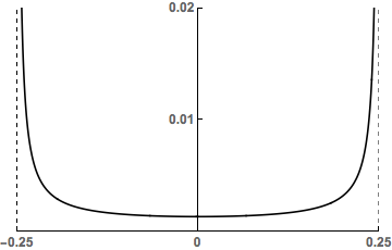
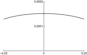
We have Φ^​(t)>0\widehat{\Phi}(t)>0 for t∈ℝ∪i(0,1/4]t\in\mathbb{R}\cup i(0,1/4]. When k=−12k=-\frac{1}{2}, the factor Dk​(t)D_{k}(t) produces a pole of Φ^\widehat{\Phi} at t=i/4t=i/4. However, this value does not occur in the sum (5.5), since this value of the spectral parameter rjr_{j} corresponds to the minimal eigenvalue λj=316\lambda_{j}=\frac{3}{16}, which does not arise by the discussion at the end of Section 2 since there are no holomorphic modular forms in negative weight. In this case every eigenvalue has λj≥14−(732)2\lambda_{j}\geq\frac{1}{4}-\left(\frac{7}{32}\right)^{2}; this follows from the discussion in [Sar84, §3] and the lower bound 14−(764)2\frac{1}{4}-\left(\frac{7}{64}\right)^{2} which is available in weight zero by the work of Kim and Sarnak [Kim03, Appendix 2].
Refer to caption
(a) Φ^​(i​t)\widehat{\Phi}(it) for t∈[−1/4,1/4]t\in[-1/4,1/4] when k=1/2k=1/2.
Refer to caption
(b) Φ^​(i​t)\widehat{\Phi}(it) for t∈(−1/4,1/4)t\in(-1/4,1/4) when k=−1/2k=-1/2.
Figure 1. Plots of Φ^​(t)\widehat{\Phi}(t) for imaginary tt.

Let n∈ℕn\in\mathbb{N} and let 𝒬\mathcal{Q} be as in (5.12). For each Q∈𝒬Q\in\mathcal{Q}, Proposition 5.1 gives

ℒΦ^(Q)​(n,n)+ℳΦ^(Q)​(n,n)=γk​𝒦Φ(Q)​(n,n)−𝒩Φˇ(Q)​(n,n).\mathcal{L}^{(Q)}_{\widehat{\Phi}}(n,n)+\mathcal{M}^{(Q)}_{\widehat{\Phi}}(n,n)=\gamma_{k}\mathcal{K}^{(Q)}_{\Phi}(n,n)-\mathcal{N}^{(Q)}_{\widecheck{\Phi}}(n,n).

From (5.5) and (5.6) we see that ℒΦ^(Q)​(n,n)\mathcal{L}^{(Q)}_{\widehat{\Phi}}(n,n) and ℳΦ^(Q)​(n,n)\mathcal{M}^{(Q)}_{\widehat{\Phi}}(n,n) are positive, from which

(5.17) ℒΦ^(Q)​(n,n)≤γk​𝒦Φ(Q)​(n,n)−𝒩Φˇ(Q)​(n,n).\mathcal{L}^{(Q)}_{\widehat{\Phi}}(n,n)\leq\gamma_{k}\mathcal{K}^{(Q)}_{\Phi}(n,n)-\mathcal{N}^{(Q)}_{\widecheck{\Phi}}(n,n).

For each Q∈𝒬Q\in\mathcal{Q}, the functions {[Γ0(N):Γ0(Q)]−12uj}\left\{[\Gamma_{0}(N):\Gamma_{0}(Q)]^{-\frac{1}{2}}u_{j}\right\} form an orthonormal subset of ℒ~k​(Q,ν)\widetilde{\mathcal{L}}_{k}(Q,\nu). Since [Γ0(N):Γ0(Q)]≤p+1≪P[\Gamma_{0}(N):\Gamma_{0}(Q)]\leq p+1\ll P, we find that

ℒΦ^(Q)(n,n)≥ℒΦ^(N)​(n,n)[Γ0(N):Γ0(Q)]≫ℒΦ^(N)​(n,n)P.\mathcal{L}^{(Q)}_{\hat{\Phi}}(n,n)\geq\frac{\mathcal{L}^{(N)}_{\hat{\Phi}}(n,n)}{[\Gamma_{0}(N):\Gamma_{0}(Q)]}\gg\frac{\mathcal{L}^{(N)}_{\hat{\Phi}}(n,n)}{P}.

Since |𝒬|≍P/log⁡P|\mathcal{Q}|\asymp P/\log P, summing (5.17) over QQ gives

(5.18) 1log⁡P​ℒΦ^(N)​(n,n)≪∑Q∈𝒬|𝒦Φ(Q)​(n,n)|+∑Q∈𝒬|𝒩Φˇ(Q)​(n,n)|.\frac{1}{\log P}\mathcal{L}^{(N)}_{\hat{\Phi}}(n,n)\ll\sum_{Q\in\mathcal{Q}}\left|\mathcal{K}^{(Q)}_{\Phi}(n,n)\right|+\sum_{Q\in\mathcal{Q}}\left|\mathcal{N}^{(Q)}_{\widecheck{\Phi}}(n,n)\right|.

As in [Iwa87] and [Duk88], we choose

P=n17.P=n^{\frac{1}{7}}.

In the next two sections we bound the right-hand side of (5.18).

5.3. Treatment of 𝒩Φˇ(Q)​(n,n)\mathcal{N}^{(Q)}_{\widecheck{\Phi}}(n,n)

When k=±12k=\pm\frac{1}{2} we have

𝒩Φˇ(Q)​(n,n)=∑ℓ≡k(mod2)ℓ>2Φˇ​(ℓ)​Γ​(ℓ)​∑f∈ℬℓ|af​(n)|2.\mathcal{N}^{(Q)}_{\widecheck{\Phi}}(n,n)=\sum_{\begin{subarray}{c}\ell\equiv k\pmod{2}\\ \ell>2\end{subarray}}\widecheck{\Phi}(\ell)\Gamma(\ell)\sum_{f\in\mathcal{B}_{\ell}}|a_{f}(n)|^{2}.

Recalling the normalization (5.7), we have Petersson’s formula (c.f. [DFI12, Proposition 2.3])

∑f∈ℬℓ|af​(n)|2=1Γ⁡(ℓ−1)​(1+2​π​i−ℓ​∑c≡0(modQ)c−1​S​(n,n,c,ν)​Jℓ−1​(4​π​nc)).\sum_{f\in\mathcal{B}_{\ell}}|a_{f}(n)|^{2}=\frac{1}{\Gamma(\ell-1)}\left(1+2\pi i^{-\ell}\sum_{c\equiv 0\pmod{Q}}c^{-1}S(n,n,c,\nu)J_{\ell-1}\left(\mathord{\raise 0.49991pt\hbox{$\displaystyle\genfrac{}{}{0.4pt}{}{4 \pi n}{c}$}}\right)\right).

Recalling the definition (5.8), we obtain

(5.19) ∑Q∈𝒬|𝒩Φˇ(Q)​(n,n)|≪P​∑ℓ≡k(mod2)ℓ>2ℓ​|Φ~​(ℓ)|+∑ℓ≡k(mod2)ℓ>2ℓ|Φ~(ℓ)|∑Q∈𝒬|∑c≡0(modQ)c−1S(n,n,c,ν)Jℓ−1(4​π​nc)|.\sum_{Q\in\mathcal{Q}}\left|\mathcal{N}^{(Q)}_{\widecheck{\Phi}}(n,n)\right|\ll P\sum_{\begin{subarray}{c}\ell\equiv k\pmod{2}\\ \ell>2\end{subarray}}\ell\,|\widetilde{\Phi}(\ell)|\\ +\sum_{\begin{subarray}{c}\ell\equiv k\pmod{2}\\ \ell>2\end{subarray}}\ell\,|\widetilde{\Phi}(\ell)|\sum_{Q\in\mathcal{Q}}\Bigg|\sum_{c\equiv 0\pmod{Q}}c^{-1}S(n,n,c,\nu)J_{\ell-1}\left(\mathord{\raise 0.49991pt\hbox{$\displaystyle\genfrac{}{}{0.4pt}{}{4 \pi n}{c}$}}\right)\Bigg|.

The first sum on the right is ≪P\ll P by (5.16). It is important to obtain bounds for the inner term which are uniform in ℓ\ell as well as nn. For small ℓ\ell we are able to control the dependence on ℓ\ell explicitly, and for large ℓ\ell we exploit the decay of Φ~​(ℓ)\widetilde{\Phi}(\ell). Let β>0\beta>0 be a parameter to be chosen later. In the next two subsections we treat the ranges ℓ≤nβ\ell\leq n^{\beta} and ℓ>nβ\ell>n^{\beta} separately.

5.3.1. Small values of ℓ\ell: ℓ≤nβ\ell\leq n^{\beta}

For these values of ℓ\ell, we treat the three ranges

1≤c≤n/ℓ2,n/ℓ2≤c≤nandc≥n.1\leq c\leq n/\ell^{2},\quad n/\ell^{2}\leq c\leq n\quad\text{and}\quad c\geq n.

In the first range we use an explicit representation for Jℓ−1​(z)J_{\ell-1}(z) when ℓ∈12​ℕ−ℕ\ell\in\frac{1}{2}\mathbb{N}-\mathbb{N}. For such ℓ\ell and for k≥0k\geq 0 define

cℓ,k:=Γ⁡(ℓ−12+k)k!​Γ​(ℓ−12−k),c_{\ell,k}:=\frac{\Gamma(\ell-\frac{1}{2}+k)}{k!\Gamma(\ell-\frac{1}{2}-k)},

and define the polynomial

Hℓ​(z):=e−π​i​(2​ℓ−1)42​π​∑k=0ℓ−32ik​cℓ,k​zk.H_{\ell}(z):=\frac{e^{-\frac{\pi i(2\ell-1)}{4}}}{2\pi}\sum_{k=0}^{\ell-\frac{3}{2}}i^{k}c_{\ell,k}z^{k}.

Using the first formula in [BE53, 7.11], a computation shows that for z∈ℝz\in\mathbb{R} and ℓ∈12​ℕ−ℕ\ell\in\frac{1}{2}\mathbb{N}-\mathbb{N} we have

(5.20) z​Jℓ−1​(2​π​z)=e⁡(z)​Hℓ​(14​π​z)+e⁡(−z)​H¯ℓ​(14​π​z).\sqrt{z}J_{\ell-1}(2\pi z)=e(z)H_{\ell}\left(\mathord{\raise 0.49991pt\hbox{$\displaystyle\genfrac{}{}{0.4pt}{}{1}{4\pi z}$}}\right)+e(-z)\overline{H}_{\ell}\left(\mathord{\raise 0.49991pt\hbox{$\displaystyle\genfrac{}{}{0.4pt}{}{1}{4\pi z}$}}\right).

Recall the definition (5.11). Using (5.20) and partial summation, we obtain

(5.21) ∑1≤c≤n/ℓ2c≡0(modQ)c−1​S​(n,n,c,ν)​Jℓ−1​(4​π​nc)\displaystyle\sum_{\begin{subarray}{c}1\leq c\leq n/\ell^{2}\\ c\equiv 0\pmod{Q}\end{subarray}}c^{-1}S(n,n,c,\nu)J_{\ell-1}\left(\frac{4\pi n}{c}\right)
=n−122​(Hℓ​(18​π​ℓ2)​K1(Q)​(n,nℓ2)+H¯ℓ​(18​π​ℓ2)​K−1(Q)​(n,nℓ2))\displaystyle=\frac{n^{-\frac{1}{2}}}{\sqrt{2}}\left(H_{\ell}\left(\frac{1}{8\pi\ell^{2}}\right)K_{1}^{(Q)}\left(n;\frac{n}{\ell^{2}}\right)+\overline{H}_{\ell}\left(\frac{1}{8\pi\ell^{2}}\right)K_{-1}^{(Q)}\left(n;\frac{n}{\ell^{2}}\right)\right)
−n−328​π​2∫1n/ℓ2H′ℓ(x8​π​n)K1(Q)(n;x)dx−n−328​π​2∫1n/ℓ2H¯′ℓ(x8​π​n)K−1(Q)(n;x)dx.\displaystyle-\frac{n^{-\frac{3}{2}}}{8\pi\sqrt{2}}\int_{1}^{n/\ell^{2}}H^{\prime}_{\ell}\left(\frac{x}{8\pi n}\right)K_{1}^{(Q)}(n;x)\,dx-\frac{n^{-\frac{3}{2}}}{8\pi\sqrt{2}}\int_{1}^{n/\ell^{2}}\overline{H}^{\prime}_{\ell}\left(\frac{x}{8\pi n}\right)K_{-1}^{(Q)}(n;x)\,dx.

For 0≤k≤ℓ−320\leq k\leq\ell-\frac{3}{2} we have

cℓ,k≤(2​ℓ)2​kk!.c_{\ell,k}\leq\frac{(2\ell)^{2k}}{k!}.

Therefore Hℓ​(18​π​ℓ2)≪1H_{\ell}\left(\frac{1}{8\pi\ell^{2}}\right)\ll 1 (the series converges as ℓ→∞\ell\rightarrow\infty), and we have

Hℓ′​(x8​π​n)≪ℓ2for 1≤x≤n/ℓ2.H^{\prime}_{\ell}\left(\frac{x}{8\pi n}\right)\ll\ell^{2}\quad\text{for }\quad 1\leq x\leq n/\ell^{2}.

Using (5.21) and Proposition 5.2 with P=n17P=n^{\frac{1}{7}} we obtain

(5.22) ∑Q∈𝒬|∑1≤c≤n/ℓ2c≡0(modQ)c−1​S​(n,n,c,ν)​Jℓ−1​(4​π​nc)|≪(ℓ−12​n37+ℓ−14​n2356)​(ℓ​n)ϵ.\sum_{Q\in\mathcal{Q}}\Bigg|\sum_{\begin{subarray}{c}1\leq c\leq n/\ell^{2}\\ c\equiv 0\pmod{Q}\end{subarray}}c^{-1}S(n,n,c,\nu)J_{\ell-1}\left(\mathord{\raise 0.49991pt\hbox{$\displaystyle\genfrac{}{}{0.4pt}{}{4 \pi n}{c}$}}\right)\Bigg|\ll\left(\ell^{-\frac{1}{2}}n^{\frac{3}{7}}+\ell^{-\frac{1}{4}}n^{\frac{23}{56}}\right)(\ell n)^{\epsilon}.

Now consider the range n/ℓ2≤c≤nn/\ell^{2}\leq c\leq n. We have [DLMF, (10.6.1)]

(5.23) 2​Jℓ−1′​(z)=Jℓ−2​(z)−Jℓ​(z).2J_{\ell-1}^{\prime}(z)=J_{\ell-2}(z)-J_{\ell}(z).

We also have a uniform bound for the JJ-Bessel function due to L. Landau [Lan00].

Proposition 5.3 (Landau).

For v>0v>0 and x>0x>0, we have

(5.24) |Jv​(x)|≤c0​x−13,\left|J_{v}(x)\right|\leq c_{0}x^{-\frac{1}{3}},

where c0=0.7857​…c_{0}=0.7857\dots.

Using Proposition 5.3 we find that

(5.25) (x−12​Jℓ−1​(4​π​nx))′≪n−13​x−76+n23​x−136.\left(x^{-\frac{1}{2}}J_{\ell-1}\left(\mathord{\raise 0.49991pt\hbox{$\displaystyle\genfrac{}{}{0.4pt}{}{4\pi n}{x}$}}\right)\right)^{\prime}\ll n^{-\frac{1}{3}}x^{-\frac{7}{6}}+n^{\frac{2}{3}}x^{-\frac{13}{6}}.

Partial summation using this bound together with Proposition 5.2 and (5.25) and a careful examination of the error terms which arise yields

(5.26) ∑Q∈𝒬|∑n/ℓ2≤c≤nc≡0(modQ)c−1​S​(n,n,c,ν)​Jℓ−1​(4​π​nc)|≪(ℓ116​n37+ℓ2512​n2356)​(ℓ​n)ϵ.\sum_{Q\in\mathcal{Q}}\Bigg|\sum_{\begin{subarray}{c}n/\ell^{2}\leq c\leq n\\ c\equiv 0\pmod{Q}\end{subarray}}c^{-1}S(n,n,c,\nu)J_{\ell-1}\left(\mathord{\raise 0.49991pt\hbox{$\displaystyle\genfrac{}{}{0.4pt}{}{4 \pi n}{c}$}}\right)\Bigg|\ll\left(\ell^{\frac{11}{6}}n^{\frac{3}{7}}+\ell^{\frac{25}{12}}n^{\frac{23}{56}}\right)(\ell n)^{\epsilon}.

For the remaining range c≥nc\geq n, the treatment of Iwaniec [Iwa87, pp. 400-401] applies uniformly in ℓ\ell. To see this, note that (5.23) and the inequality |Jℓ−1​(x)|≤xℓ−1Γ⁡(ℓ−1)|J_{\ell-1}(x)|\leq\frac{x^{\ell-1}}{\Gamma(\ell-1)} for x>0x>0 [DLMF, (10.14.4)] give the estimate

(5.27) (x−12​Jℓ−1​(4​π​nx))′≪n​x−52for x≥n\left(x^{-\frac{1}{2}}J_{\ell-1}\left(\mathord{\raise 0.49991pt\hbox{$\displaystyle\genfrac{}{}{0.4pt}{}{4\pi n}{x}$}}\right)\right)^{\prime}\ll nx^{-\frac{5}{2}}\quad\text{for }\quad x\geq n

which is used in that argument. We conclude that for all ℓ\ell we have

(5.28) ∑Q∈𝒬|∑c≥nc≡0(modQ)c−1​S​(n,n,c,ν)​Jℓ−1​(4​π​nc)|≪n37+ϵ.\sum_{Q\in\mathcal{Q}}\Bigg|\sum_{\begin{subarray}{c}c\geq n\\ c\equiv 0\pmod{Q}\end{subarray}}c^{-1}S(n,n,c,\nu)J_{\ell-1}\left(\mathord{\raise 0.49991pt\hbox{$\displaystyle\genfrac{}{}{0.4pt}{}{4 \pi n}{c}$}}\right)\Bigg|\ll n^{\frac{3}{7}+\epsilon}.

From (5.16), (5.22), (5.26) and (5.28) we obtain

(5.29) ∑ℓ≡k(mod2)2<ℓ≤nβℓ​|Φ~​(ℓ)|​∑Q∈𝒬|∑c≡0(modQ)c−1​S​(n,n,c,ν)​Jℓ−1​(4​π​nc)|≪∑2<ℓ≤nβℓ−2​(ℓ116​n37+ℓ2512​n2356)​(ℓ​n)ϵ≪n37+56​β+ϵ+n2356+1312​β+ϵ.\sum_{\begin{subarray}{c}\ell\equiv k\pmod{2}\\ 2<\ell\leq n^{\beta}\end{subarray}}\ell\,|\widetilde{\Phi}(\ell)|\sum_{Q\in\mathcal{Q}}\Bigg|\sum_{c\equiv 0\pmod{Q}}c^{-1}S(n,n,c,\nu)J_{\ell-1}\left(\mathord{\raise 0.49991pt\hbox{$\displaystyle\genfrac{}{}{0.4pt}{}{4 \pi n}{c}$}}\right)\Bigg|\\ \ll\sum_{2<\ell\leq n^{\beta}}\ell^{-2}\left(\ell^{\frac{11}{6}}n^{\frac{3}{7}}+\ell^{\frac{25}{12}}n^{\frac{23}{56}}\right)(\ell n)^{\epsilon}\ll n^{\frac{3}{7}+\frac{5}{6}\beta+\epsilon}+n^{\frac{23}{56}+\frac{13}{12}\beta+\epsilon}.

5.3.2. Large values of ℓ\ell: ℓ>nβ\ell>n^{\beta}

Let 0<γ<10<\gamma<1 be a parameter to be chosen later. We consider the three ranges

1≤c≤nγ,nγ≤c≤n,andc≥n.1\leq c\leq n^{\gamma},\quad n^{\gamma}\leq c\leq n,\quad\text{and}\quad c\geq n.

We begin with a simple lemma.

Lemma 5.4.

Let 𝒬\mathcal{Q} be as in (5.12). For b>−1b>-1 we have

∑Q∈𝒬∑c≤xc≡0(modQ)cb(n,c)12≪ϵxb+1nϵlogP.\sum_{Q\in\mathcal{Q}}\sum_{\begin{subarray}{c}c\leq x\\ c\equiv 0\pmod{Q}\end{subarray}}c^{b}(n,c)^{\frac{1}{2}}\ll_{\epsilon}x^{b+1}n^{\epsilon}\log P.
Proof.

The inner sum is

≤∑d|nd12​∑c≤xc≡0(mod[d,Q])cb≪xb+1​∑d|nd12[d,Q]≤xb+1​(n,N)Q​∑d|n1d12≪xb+1​NQ​nϵ,\leq\sum_{d\mid n}d^{\frac{1}{2}}\!\!\!\!\!\!\sum_{\begin{subarray}{c}c\leq x\\ c\equiv 0\pmod{[d,Q]}\end{subarray}}c^{b}\ll x^{b+1}\sum_{d\mid n}\frac{d^{\frac{1}{2}}}{[d,Q]}\leq x^{b+1}\frac{(n,N)}{Q}\sum_{d\mid n}\frac{1}{d^{\frac{1}{2}}}\ll x^{b+1}\frac{N}{Q}n^{\epsilon},

where we have used the fact that such QQ have Q=p​NQ=pN with p∤np\nmid n. Writing Q=p​NQ=pN and summing over pp gives the lemma. ∎

In the first range, we estimate using the Weil bound (5.10), Proposition 5.3, and Lemma 5.4. We obtain

(5.30) ∑Q∈𝒬|∑1≤c≤nγc≡0(modQ)c−1​S​(n,n,c,ν)​Jℓ−1​(4​π​nc)|≪∑Q∈𝒬n−13​∑1≤c≤nγc≡0(modQ)c−16​(n,c)12≪n56​γ−13+ϵ.\sum_{Q\in\mathcal{Q}}\Bigg|\sum_{\begin{subarray}{c}1\leq c\leq n^{\gamma}\\ c\equiv 0\pmod{Q}\end{subarray}}c^{-1}S(n,n,c,\nu)J_{\ell-1}\left(\mathord{\raise 0.49991pt\hbox{$\displaystyle\genfrac{}{}{0.4pt}{}{4 \pi n}{c}$}}\right)\Bigg|\ll\sum_{Q\in\mathcal{Q}}n^{-\frac{1}{3}}\sum_{\begin{subarray}{c}1\leq c\leq n^{\gamma}\\ c\equiv 0\pmod{Q}\end{subarray}}c^{-\frac{1}{6}}(n,c)^{\frac{1}{2}}\ll n^{\frac{5}{6}\gamma-\frac{1}{3}+\epsilon}.

In the second range we use partial summation together with Proposition 5.2 and (5.25). Examining the error terms which arise from this computation, we obtain

(5.31) ∑Q∈𝒬|∑nγ≤c≤nc≡0(modQ)c−1​S​(n,n,c,ν)​Jℓ−1​(4​π​nc)|≪(n37+n6142−2524​γ+n11384−1112​γ+n2542−16​γ+n1942−124​γ+n2984+112​γ+n−1742+56​γ)​nϵ.\sum_{Q\in\mathcal{Q}}\Bigg|\sum_{\begin{subarray}{c}n^{\gamma}\leq c\leq n\\ c\equiv 0\pmod{Q}\end{subarray}}c^{-1}S(n,n,c,\nu)J_{\ell-1}\left(\mathord{\raise 0.49991pt\hbox{$\displaystyle\genfrac{}{}{0.4pt}{}{4 \pi n}{c}$}}\right)\Bigg|\\ \ll\left(n^{\frac{3}{7}}+n^{\frac{61}{42}-\frac{25}{24}\gamma}+n^{\frac{113}{84}-\frac{11}{12}\gamma}+n^{\frac{25}{42}-\frac{1}{6}\gamma}+n^{\frac{19}{42}-\frac{1}{24}\gamma}+n^{\frac{29}{84}+\frac{1}{12}\gamma}+n^{-\frac{17}{42}+\frac{5}{6}\gamma}\right)n^{\epsilon}.

For the third range we recall that (5.28) holds for all ℓ\ell.

We choose γ=4749\gamma=\frac{47}{49} to balance (5.30) and (5.31) (this is the value for which 11384−1112​γ=56​γ−13\frac{113}{84}-\frac{11}{12}\gamma=\frac{5}{6}\gamma-\frac{1}{3}). For this range of ℓ\ell we obtain

(5.32) ∑Q∈𝒬|∑nγ≤c≤nc≡0(modQ)c−1​S​(n,n,c,ν)​Jℓ−1​(4​π​nc)|≪n137294+ϵ,\sum_{Q\in\mathcal{Q}}\Bigg|\sum_{\begin{subarray}{c}n^{\gamma}\leq c\leq n\\ c\equiv 0\pmod{Q}\end{subarray}}c^{-1}S(n,n,c,\nu)J_{\ell-1}\left(\mathord{\raise 0.49991pt\hbox{$\displaystyle\genfrac{}{}{0.4pt}{}{4 \pi n}{c}$}}\right)\Bigg|\ll n^{\frac{137}{294}+\epsilon},

from which

(5.33) ∑ℓ≡k(mod2)ℓ>nβℓ​|Φ~​(ℓ)|​∑Q∈𝒬|∑c≡0(modQ)c−1​S​(n,n,c,ν)​Jℓ−1​(4​π​nc)|≪n137294+ϵ​∑ℓ>nβℓ−2≪n137294−β+ϵ.\sum_{\begin{subarray}{c}\ell\equiv k\pmod{2}\\ \ell>n^{\beta}\end{subarray}}\ell|\widetilde{\Phi}(\ell)|\sum_{Q\in\mathcal{Q}}\Bigg|\sum_{c\equiv 0\pmod{Q}}c^{-1}S(n,n,c,\nu)J_{\ell-1}\left(\mathord{\raise 0.49991pt\hbox{$\displaystyle\genfrac{}{}{0.4pt}{}{4 \pi n}{c}$}}\right)\Bigg|\\ \ll n^{\frac{137}{294}+\epsilon}\sum_{\ell>n^{\beta}}\ell^{-2}\ll n^{\frac{137}{294}-\beta+\epsilon}.

Finally, we choose β=149\beta=\frac{1}{49} to balance (5.29) and (5.33). From (5.19), we obtain

(5.34) ∑Q∈𝒬|𝒩Φˇ(Q)​(n,n)|≪n131294+ϵ.\sum_{Q\in\mathcal{Q}}\left|\mathcal{N}^{(Q)}_{\widecheck{\Phi}}(n,n)\right|\ll n^{\frac{131}{294}+\epsilon}.

5.4. Treatment of 𝒦Φ(Q)​(n,n)\mathcal{K}_{\Phi}^{(Q)}(n,n)

From the definition (5.4) we have

(5.35) ∑Q∈𝒬|𝒦Φ(Q)​(n,n)|≪n−12​∑Q∈𝒬|∑c≤nc≡0(modQ)c−12​S​(n,n,c,ν)​J92​(4​π​nc)|+n−12∑Q∈𝒬|∑c>nc≡0(modQ)c−12S(n,n,c,ν)J92(4​π​nc)|.\sum_{Q\in\mathcal{Q}}\left|\mathcal{K}_{\Phi}^{(Q)}(n,n)\right|\ll n^{-\frac{1}{2}}\sum_{Q\in\mathcal{Q}}\Bigg|\sum_{\begin{subarray}{c}c\leq n\\ c\equiv 0\pmod{Q}\end{subarray}}c^{-\frac{1}{2}}S(n,n,c,\nu)J_{\frac{9}{2}}\left(\mathord{\raise 0.49991pt\hbox{$\displaystyle\genfrac{}{}{0.4pt}{}{4 \pi n}{c}$}}\right)\Bigg|\\ +n^{-\frac{1}{2}}\sum_{Q\in\mathcal{Q}}\Bigg|\sum_{\begin{subarray}{c}c>n\\ c\equiv 0\pmod{Q}\end{subarray}}c^{-\frac{1}{2}}S(n,n,c,\nu)J_{\frac{9}{2}}\left(\mathord{\raise 0.49991pt\hbox{$\displaystyle\genfrac{}{}{0.4pt}{}{4 \pi n}{c}$}}\right)\Bigg|.

Here the situation is simpler since the JJ-Bessel function has fixed order. For the first term, we use the expression (5.20) and partial summation with Proposition 5.2, together with the fact that (x12​H112​(x8​π​n))′≪x−12+x12​n−1\left(x^{\frac{1}{2}}H_{\frac{11}{2}}\left(\frac{x}{8\pi n}\right)\right)^{\prime}\ll x^{-\frac{1}{2}}+x^{\frac{1}{2}}n^{-1} for 1≤x≤n1\leq x\leq n. For the second term, (5.23) and [DLMF, (10.14.4)] give (J92​(4​π​nx))′≪n92​x−112\left(J_{\frac{9}{2}}\left(\frac{4\pi n}{x}\right)\right)^{\prime}\ll n^{\frac{9}{2}}x^{\frac{-11}{2}} for x≥nx\geq n. We conclude that

(5.36) ∑Q∈𝒬|𝒦Φ(Q)​(n,n)|≪n37+ϵ.\sum_{Q\in\mathcal{Q}}\left|\mathcal{K}_{\Phi}^{(Q)}(n,n)\right|\ll n^{\frac{3}{7}+\epsilon}.

5.5. Proof of Theorem 4.3

From (5.18), (5.34) and (5.36) we have

ℒΦ^(N)​(n,n)≪n131294+ϵ.\mathcal{L}^{(N)}_{\hat{\Phi}}(n,n)\ll n^{\frac{131}{294}+\epsilon}.

Until now we have assumed that N≡0(mod8)N\equiv 0\pmod{8}, but we may drop this assumption using positivity after replacing NN by 2​N2N if necessary. The last inequality gives

(5.37) n​∑j≥0|ρj​(n)|2​Φ^​(rj)ch⁡π​rj≪n131294+ϵ.n\sum_{j\geq 0}\left|\rho_{j}(n)\right|^{2}\frac{\widehat{\Phi}(r_{j})}{\ch\pi r_{j}}\ll n^{\frac{131}{294}+\epsilon}.

From the asymptotics of the Gamma function [DLMF, (5.11.9)], for k=±12k=\pm\frac{1}{2} we have

(5.38) Φ^​(t)≫tk−3for t≥1.\widehat{\Phi}(t)\gg t^{k-3}\qquad\text{for $t\geq 1$}.

By the discussion in Section 5.2, there are positive constants c1c_{1} and c2c_{2} such that for each rj∈[0,1]∪i(0,1/4]r_{j}\in[0,1]\cup i(0,1/4] which appears in the sum (5.37) we have

(5.39) c1≤Φ^​(rj)≤c2.c_{1}\leq\widehat{\Phi}(r_{j})\leq c_{2}.

So for every rjr_{j} which appears in the sum, we have

(5.40) Φ^​(rj)−1≪λj3−k2.\widehat{\Phi}(r_{j})^{-1}\ll\lambda_{j}^{\frac{3-k}{2}}.

Suppose that x≥1x\geq 1. We have xk−3​Φ^−1​(rj)≪1x^{k-3}\hat{\Phi}^{-1}(r_{j})\ll 1 for 1≤rj≤x1\leq r_{j}\leq x by (5.38). The same bound holds for |rj|≤1|r_{j}|\leq 1 by (5.39). Therefore (5.37) gives the average estimate

(5.41) n​∑|rj|≤x|ρj​(n)|2ch⁡π​rj≪x3−k​n131294+ϵ.n\sum_{|r_{j}|\leq x}\frac{|\rho_{j}(n)|^{2}}{\ch\pi r_{j}}\ll x^{3-k}n^{\frac{131}{294}+\epsilon}.

Suppose now that k=12k=\frac{1}{2} as in the statement of Theorem 4.3. When n>0n>0, the theorem follows directly from (5.41). When n<0n<0 it follows from the relationship (2.11).

6. Kuznetsov trace formula in the mixed-sign case

We give a version of the Kusnetsov trace formula in the mixed sign case which is suitable for our applications. Suppose that ϕ:[0,∞)→ℂ\phi:[0,\infty)\rightarrow\mathbb{C} is four times continuously differentiable and satisfies

(6.1) ϕ(0)=ϕ′(0)=0,ϕ(j)(x)≪ϵx−2−ϵ(j=0,…,4)asx→∞,\phi(0)=\phi^{\prime}(0)=0,\quad\phi^{(j)}(x)\ll_{\epsilon}x^{-2-\epsilon}\quad(j=0,\ldots,4)\quad\text{as}\quad x\rightarrow\infty,

for some ϵ>0\epsilon>0. Define the transform

(6.2) ϕˇ​(r):=ch⁡π​r​∫0∞K2​i​r​(u)​ϕ​(u)​d​uu\widecheck{\phi}(r):=\ch\pi r\int_{0}^{\infty}K_{2ir}(u)\phi(u)\frac{du}{u}

(we use the notation ϕ\phi instead of Φ\Phi for the rest of the paper to avoid potential confusion with the transform defined in the last section).

Suppose that NN is a positive integer and that ν\nu is a multiplier of weight 12\frac{1}{2} for Γ0​(N)\Gamma_{0}(N) with the property that no cusp is singular with respect to ν\nu. In this case the Kusnetsov formula has a relatively simple expression since there are no Eisenstein series and there is no contribution from cusp forms due to the mixed sign of the arguments. A proof of the following result is given in Section 4 of [AA18] in the case when ν\nu is the multiplier on SL2​(ℤ){\rm SL}_{2}(\mathbb{Z}) associated to the Dedekind eta function (in this case there is no residual spectrum). The general case follows by this argument with only cosmetic changes. Blomer [Blo08] has proved a version of this formula for the twisted theta-multiplier.

Proposition 6.1.

Let ν\nu be a multiplier of weight 12\frac{1}{2} for Γ0​(N)\Gamma_{0}(N) such that no cusp is singular with respect to ν\nu. Let ρj​(n)\rho_{j}(n) denote the coefficients of an orthonormal basis {vj​(τ)}\{v_{j}(\tau)\} for ℒ~12​(N,ν)\widetilde{\mathcal{L}}_{\frac{1}{2}}(N,\nu). Suppose that ϕ\phi satisfies conditions (6.1). If mν>0m_{\nu}>0 and nν<0n_{\nu}<0 then

∑c>0c≡0(modN)S⁡(m,n,c,ν)c​ϕ​(4​π​mν​|nν|c)=8​i​mν​|nν|​∑rjρj​(m)¯​ρj​(n)ch⁡π​rj​ϕˇ​(rj).\sum_{\begin{subarray}{c}c>0\\ c\equiv 0\pmod{N}\end{subarray}}\frac{S(m,n,c,\nu)}{c}\phi\left(\frac{4\pi\sqrt{m_{\nu}|n_{\nu}|}}{c}\right)=8\sqrt{i}\sqrt{m_{\nu}|n_{\nu}|}\sum_{r_{j}}\frac{\overline{\rho_{j}(m)}\rho_{j}(n)}{\ch\pi r_{j}}\widecheck{\phi}(r_{j}).

We describe a family of test functions. Given a,x>0a,x>0, let T>0T>0 be a parameter with

(6.3) T≤x/3,T≍x1−δwith0<δ<1/2.T\leq x/3,\quad T\asymp x^{1-\delta}\quad\text{with}\quad 0<\delta<1/2.

Let ϕ=ϕa,x,T:[0,∞)→[0,1]\phi=\phi_{a,x,T}:[0,\infty)\rightarrow[0,1] be a smooth function (as in [ST09] and [AA18]) satisfying

  1.   (i)

    The conditions in (6.1),

  2.   (ii)

    ϕ⁡(t)=1\phi(t)=1 for a2​x≤t≤ax\frac{a}{2x}\leq t\leq\frac{a}{x},

  3.   (iii)

    ϕ⁡(t)=0\phi(t)=0 for t≤a2​x+2​Tt\leq\frac{a}{2x+2T} and t≥ax−Tt\geq\frac{a}{x-T},

  4.   (iv)

    ϕ′​(t)≪(ax−T−ax)−1≪x2a​T\phi^{\prime}(t)\ll\left(\frac{a}{x-T}-\frac{a}{x}\right)^{-1}\ll\frac{x^{2}}{aT},

  5.   (v)

    ϕ\phi and ϕ′\phi^{\prime} are piecewise monotone on a fixed number of intervals.

We require bounds for ϕˇ\widecheck{\phi} which are recorded in [AA18, Theorem 6.1].

Proposition 6.2.

Let a,x,T be as above and let ϕ=ϕa,x,T\phi=\phi_{a,x,T}. Then

ϕˇ​(r)≪{r−32​e−r2​f​o​r1≤r≤a8​x,r−1​f​o​rmax⁡(1,a8​x)≤r≤ax,min⁡(r−32,r−52​xT)​f​o​rr≥max⁡(ax,1).\widecheck{\phi}(r)\ll\begin{cases}r^{-\frac{3}{2}}e^{-\frac{r}{2}}&\emph{for}\quad 1\leq r\leq\frac{a}{8x},\\ r^{-1}&\emph{for}\quad\max\left(1,\frac{a}{8x}\right)\leq r\leq\frac{a}{x},\\ \min\left(r^{-\frac{3}{2}},r^{-\frac{5}{2}}\frac{x}{T}\right)&\emph{for}\quad r\geq\max\left(\frac{a}{x},1\right).\end{cases}

7. Proof of Theorem 1.1

Let ψ\psi be the multiplier defined in (3.4). Theorem 1.1 will follow from a uniform estimate for sums of Kloosterman sums attached to ψ\psi. We note that many of the terms xϵx^{\epsilon} could be changed to log⁡x\log x factors if necessary, but for simplicity we do not keep track of these here.

Theorem 7.1.

Suppose that 24​n−124n-1 is positive and squarefree and that 0<δ<1/20<\delta<1/2. For X≥1X\geq 1 and ϵ>0\epsilon>0 we have

(7.1) ∑c≤Xc≡0(mod2)S⁡(0,n,c,ψ)c≪δ,ϵ(n1356+ϵX34​δ+n143588+ϵ+X12−δ)Xϵ.\sum_{\begin{subarray}{c}c\leq X\\ c\equiv 0\pmod{2}\end{subarray}}\frac{S(0,n,c,\psi)}{c}\ll_{\delta,\epsilon}\left(n^{\frac{13}{56}+\epsilon}X^{\frac{3}{4}\delta}+n^{\frac{143}{588}+\epsilon}+X^{\frac{1}{2}-\delta}\right)X^{\epsilon}.

This follows in turn from an estimate over dyadic ranges.

Proposition 7.2.

Suppose that 24​n−124n-1 is positive and squarefree and that 0<δ<1/20<\delta<1/2. For x≥1x\geq 1 and ϵ>0\epsilon>0 we have

∑x≤c≤2​xc≡0(mod2)S⁡(0,n,c,ψ)c≪δ,ϵn143147+ϵx−32+n1356x34​δ+ϵ+x12−δ+ϵ.\sum_{\begin{subarray}{c}x\leq c\leq 2x\\ c\equiv 0\pmod{2}\end{subarray}}\frac{S(0,n,c,\psi)}{c}\ll_{\delta,\epsilon}n^{\frac{143}{147}+\epsilon}x^{-\frac{3}{2}}+n^{\frac{13}{56}}x^{\frac{3}{4}\delta+\epsilon}+x^{\frac{1}{2}-\delta+\epsilon}.

We show that Proposition 7.2 implies Theorem 7.1. Corollary 9.2 below gives a Weil bound for the individual Kloosterman sums, so the initial segment 1≤c≤n1432941\leq c\leq n^{\frac{143}{294}} contributes O⁡(n143588+ϵ)O\left(n^{\frac{143}{588}+\epsilon}\right) to (7.1). One can then break the interval n143294≤c≤Xn^{\frac{143}{294}}\leq c\leq X into O⁡(log⁡X)O(\log X) dyadic intervals x≤c≤2​xx\leq c\leq 2x with n143294≤x≤X/2n^{\frac{143}{294}}\leq x\leq X/2 and use Proposition 7.2 for each interval.

Proof of Proposition 7.2.

Let {uj​(τ)}\{u_{j}(\tau)\} be an orthonormal basis for ℒ~12​(2,ψ)\widetilde{\mathcal{L}}_{\frac{1}{2}}(2,\psi) with Fourier coefficients ρj​(n)\rho_{j}(n) and eigenvalues λj=14+rj2\lambda_{j}=\frac{1}{4}+r_{j}^{2}. Recall that αψ=124\alpha_{\psi}=\frac{1}{24}, so that nψ=n−124n_{\psi}=n-\frac{1}{24}, and define

(7.2) a:=2​π6​nψ.a:=\frac{2\pi}{\sqrt{6}}\sqrt{n_{\psi}}.

Let ϕ=ϕa,x,T:[0,∞)→ℝ\phi=\phi_{a,x,T}:[0,\infty)\rightarrow\mathbb{R} be a smooth test function with the properties listed in Section 6.

Using Corollary 9.2 and recalling the definition (6.3) of TT we obtain

(7.3) |∑c>0c≡0(mod2)S⁡(0,n,c,ψ)c​ϕ​(ac)−∑x≤c≤2​xc≡0(mod2)S⁡(0,n,c,ψ)c|≤∑x−T≤c≤x2​x≤c≤2​x+2​T|S⁡(0,n,c,ψ)|c≪δx12−δlogx.\left|\sum_{\begin{subarray}{c}c>0\\ c\equiv 0\pmod{2}\end{subarray}}\frac{S(0,n,c,\psi)}{c}\phi\left(\frac{a}{c}\right)-\sum_{\begin{subarray}{c}x\leq c\leq 2x\\ c\equiv 0\pmod{2}\end{subarray}}\frac{S(0,n,c,\psi)}{c}\right|\\ \leq\sum_{\begin{subarray}{c}x-T\leq c\leq x\\ 2x\leq c\leq 2x+2T\end{subarray}}\frac{|S(0,n,c,\psi)|}{c}\ll_{\delta}x^{\frac{1}{2}-\delta}\log x.

We now estimate the smoothed sums. Proposition 6.1 gives

(7.4) ∑c>0c≡0(mod2)S⁡(0,n,c,ψ)c​ϕ​(ac)=4​i6​nψ​∑rjρj​(0)¯​ρj​(n)ch⁡π​rj​ϕˇ​(rj).\sum_{\begin{subarray}{c}c>0\\ c\equiv 0\pmod{2}\end{subarray}}\frac{S(0,n,c,\psi)}{c}\phi\left(\frac{a}{c}\right)=\frac{4\sqrt{i}}{\sqrt{6}}\sqrt{n_{\psi}}\sum_{r_{j}}\frac{\overline{\rho_{j}(0)}\rho_{j}(n)}{\ch\pi r_{j}}\widecheck{\phi}(r_{j}).

If f⁡(τ)∈ℒ~12​(2,ψ)f(\tau)\in\widetilde{\mathcal{L}}_{\frac{1}{2}}(2,\psi) has minimal eigenvalue λ=316\lambda=\frac{3}{16}, then by the discussion in Section 2 y14​f​(24​τ)∈M12​(144,(12∙)​νθ)y^{\frac{1}{4}}f(24\tau)\in M_{\frac{1}{2}}\left(144,\left(\frac{12}{\bullet}\right)\nu_{\theta}\right). By the Serre-Stark basis theorem [SS77], this space is spanned by θ⁡(12​τ)=1+⋯\theta(12\tau)=1+\cdots. In view of the Fourier expansion (2.10) this minimal eigenvalue does not occur, so each form uju_{j} appearing in (7.4) is cuspidal. Applying a lift of Sarnak [Sar84, §3] such a form implies the existence of a non-zero form in the discrete spectrum in ℒ0​(72,𝟏)\mathcal{L}_{0}(72,\mathbf{1}) with eigenvalue 4​λj−34>04\lambda_{j}-\frac{3}{4}>0 (the map λj↦4​λj−34\lambda_{j}\mapsto 4\lambda_{j}-\frac{3}{4} corresponds to the map rj↦2​rjr_{j}\mapsto 2r_{j}). The image of uju_{j} under this lift must therefore be a cusp form (since the residual spectrum occurs only when λ=0\lambda=0 for congruence groups). From the numerical data in the L-series and modular forms database [LMF13] we see that 2​rj>1.12r_{j}>1.1. It follows that rj>12r_{j}>\frac{1}{2} for all jj in the sum (7.4).

After this discussion we break the sum (7.4) into three ranges dictated by the behavior of ϕˇ\widecheck{\phi} in Proposition 6.2. These are

(7.5) 0.5<rj≤a8​x,max(1,a8​x)<rj<ax,andrj≥max(1,ax).0.5<r_{j}\leq\frac{a}{8x},\qquad\max\left(1,\frac{a}{8x}\right)<r_{j}<\frac{a}{x},\qquad\text{and}\quad r_{j}\geq\max\left(1,\frac{a}{x}\right).

Let vj​(τ):=uj​(24​τ)v_{j}(\tau):=u_{j}(24\tau). After multiplication by a fixed constant, Lemma 3.2 shows that {vj​(τ)}\{v_{j}(\tau)\} is an orthonormal subset of ℒ~12​(144,(12∙)​νθ)\widetilde{\mathcal{L}}_{\frac{1}{2}}\left(144,\left(\frac{12}{\bullet}\right)\nu_{\theta}\right). Denote the Fourier coefficients of vj​(τ)v_{j}(\tau) by bj​(n)b_{j}(n), so that

(7.6) ρj​(n)=bj​(24​n−1).\rho_{j}(n)=b_{j}(24n-1).

By a straightforward argument using the Weil bound (5.10) for the sums S⁡(n,n,c,(12∙)​νθ)S\left(n,n,c,\left(\frac{12}{\bullet}\right)\nu_{\theta}\right), (4.1) is satisfied with the choice β=12+ϵ\beta=\frac{1}{2}+\epsilon. Using (7.6) and Proposition 4.1 we obtain

(7.7) ρj​(0)ch⁡π​rj=bj​(−1)ch⁡π​rj≪rj54,\frac{\rho_{j}(0)}{\sqrt{\ch\pi r_{j}}}=\frac{b_{j}(-1)}{\sqrt{\ch\pi r_{j}}}\ll r_{j}^{\frac{5}{4}},

while Proposition 4.2 and (7.6) give

(7.8) ρj​(n)ch⁡π​rj=bj​(24​n−1)ch⁡π​rj≪n−27+ϵ​rj94.\frac{\rho_{j}(n)}{\sqrt{\ch\pi r_{j}}}=\frac{b_{j}(24n-1)}{\sqrt{\ch\pi r_{j}}}\ll n^{-\frac{2}{7}+\epsilon}r_{j}^{\frac{9}{4}}.

Using Proposition 6.2, (7.7) and (7.8) we obtain

(7.9) nψ​∑0.5<rj≤a8​x|ρj​(0)¯​ρj​(n)ch⁡π​rj​ϕˇ​(rj)|≪n314+ϵ​(∑0.5<rj≤1|ϕˇ​(rj)|+∑1≤rj≤a8​xrj2​e−rj2)≪n314+ϵ.\sqrt{n_{\psi}}\sum_{0.5<r_{j}\leq\frac{a}{8x}}\left|\frac{\overline{\rho_{j}(0)}\rho_{j}(n)}{\ch\pi r_{j}}\widecheck{\phi}(r_{j})\right|\ll n^{\frac{3}{14}+\epsilon}\left(\sum_{0.5<r_{j}\leq 1}|\widecheck{\phi}(r_{j})|+\sum_{1\leq r_{j}\leq\frac{a}{8x}}r_{j}^{2}e^{-\frac{r_{j}}{2}}\right)\ll n^{\frac{3}{14}+\epsilon}.

To obtain the last estimate we use the fact that the first sum on the right contains only finitely many terms, so it is O⁡(1)O(1) by (6.2) and [DLMF, (10.25.3)]. The second sum is also O⁡(1)O(1) by Weyl’s law for the multiplier ψ\psi [Hej76, Theorem 2.28, p. 414].

Note that the results in Section 4 apply to the orthonormal collection {vj​(τ)}\{v_{j}(\tau)\} by positivity. Using the Cauchy-Schwarz inequality, Proposition 4.1, Theorem 4.3, and Proposition 6.2, we obtain

(7.10) nψ​∑a8​x≤rj<ax|ρj​(0)¯​ρj​(n)ch⁡π​rj​ϕˇ​(rj)|≪(∑a8​x≤rj<ax|bj​(−1)|2ch⁡π​rj)12×(nψ​∑a8​x≤rj<ax|bj​(24​n−1)|2ch⁡π​rj​|ϕˇ​(rj)|2)12≪n131588+ϵ​(ax)32≪n143147+ϵ​x−32.\sqrt{n_{\psi}}\sum_{\frac{a}{8x}\leq r_{j}<\frac{a}{x}}\left|\frac{\overline{\rho_{j}(0)}\rho_{j}(n)}{\ch\pi r_{j}}\widecheck{\phi}(r_{j})\right|\ll\left(\sum_{\frac{a}{8x}\leq r_{j}<\frac{a}{x}}\frac{|b_{j}(-1)|^{2}}{\ch\pi r_{j}}\right)^{\frac{1}{2}}\\ \times\left(n_{\psi}\sum_{\frac{a}{8x}\leq r_{j}<\frac{a}{x}}\frac{|b_{j}(24n-1)|^{2}}{\ch\pi r_{j}}|\widecheck{\phi}(r_{j})|^{2}\right)^{\frac{1}{2}}\ll n^{\frac{131}{588}+\epsilon}\left(\frac{a}{x}\right)^{\frac{3}{2}}\ll n^{\frac{143}{147}+\epsilon}x^{-\frac{3}{2}}.

We record two estimates which are required for the range rj≥axr_{j}\geq\frac{a}{x}. Proposition 4.1 gives

(7.11) nψ​∑0≤rj≤X|ρj​(0)¯​ρj​(n)ch⁡π​rj|≪(∑0≤rj≤X|bj​(−1)|2ch⁡π​rj)12​(nψ​∑0≤rj≤X|bj​(24​n−1)|2ch⁡π​rj)12≪(X2+n14+ϵ​X)​log⁡X,\sqrt{n_{\psi}}\sum_{0\leq r_{j}\leq X}\left|\frac{\overline{\rho_{j}(0)}\rho_{j}(n)}{\ch\pi r_{j}}\right|\ll\left(\sum_{0\leq r_{j}\leq X}\frac{|b_{j}(-1)|^{2}}{\ch\pi r_{j}}\right)^{\frac{1}{2}}\left(n_{\psi}\sum_{0\leq r_{j}\leq X}\frac{|b_{j}(24n-1)|^{2}}{\ch\pi r_{j}}\right)^{\frac{1}{2}}\\ \ll\left(X^{2}+n^{\frac{1}{4}+\epsilon}X\right)\log X,

while the same argument using Proposition 4.1 and Proposition 4.2 together gives

(7.12) nψ​∑0≤rj≤X|ρj​(0)¯​ρj​(n)ch⁡π​rj|≪(X72​n314+ϵ)​log⁡X.\sqrt{n_{\psi}}\sum_{0\leq r_{j}\leq X}\left|\frac{\overline{\rho_{j}(0)}\rho_{j}(n)}{\ch\pi r_{j}}\right|\ll\left(X^{\frac{7}{2}}n^{\frac{3}{14}+\epsilon}\right)\log X.

Let A≥max⁡(ax,1)A\geq\max\left(\frac{a}{x},1\right) and consider the dyadic range A≤rj≤2​AA\leq r_{j}\leq 2A. Using the Cauchy–Schwarz inequality, (7.11), (7.12) and Proposition 6.2 we obtain

nψ​∑A≤rj≤2​A|ρj​(0)¯​ρj​(n)ch⁡π​rj​ϕˇ​(rj)|\displaystyle\sqrt{n_{\psi}}\sum_{A\leq r_{j}\leq 2A}\left|\frac{\overline{\rho_{j}(0)}\rho_{j}(n)}{\ch\pi r_{j}}\widecheck{\phi}(r_{j})\right| ≪min⁡(A−32,A−52​xT)⋅min⁡(A2+n14+ϵ​A,n314+ϵ​A72)​log​A\displaystyle\ll\min\left(A^{-\frac{3}{2}},A^{-\frac{5}{2}}\frac{x}{T}\right)\cdot\min\left(A^{2}+n^{\frac{1}{4}+\epsilon}A,n^{\frac{3}{14}+\epsilon}A^{\frac{7}{2}}\right)\log A
≪min⁡(A12,A−12​xT)⋅min⁡(1+n14+ϵ​A−1,n314+ϵ​A32)​log​A\displaystyle\ll\min\left(A^{\frac{1}{2}},A^{-\frac{1}{2}}\frac{x}{T}\right)\cdot\min\left(1+n^{\frac{1}{4}+\epsilon}A^{-1},n^{\frac{3}{14}+\epsilon}A^{\frac{3}{2}}\right)\log A
≪n1356+ϵ​min⁡(A34,A−14​xT)​log⁡A,\displaystyle\ll n^{\frac{13}{56}+\epsilon}\min\left(A^{\frac{3}{4}},A^{-\frac{1}{4}}\frac{x}{T}\right)\log A,

where we have used

min⁡(B+C,D)≤min⁡(B,D)+min⁡(C,D)andmin⁡(B,C)≤B​C\min(B+C,D)\leq\min(B,D)+\min(C,D)\qquad\text{and}\qquad\min(B,C)\leq\sqrt{BC}

for positive B,CB,C and DD. Summing over dyadic integrals yields

(7.13) nψ∑rj≥max⁡(a/x,1)|ρj​(0)¯​ρj​(n)ch⁡(π​rj)ϕˇ(rj)|≪n1356+ϵ(xT)34+ϵ≪δn1356+ϵx34​δ+ϵ.\sqrt{n_{\psi}}\sum_{r_{j}\geq\max(a/x,1)}\left|\frac{\overline{\rho_{j}(0)}\rho_{j}(n)}{\ch(\pi r_{j})}\widecheck{\phi}(r_{j})\right|\ll n^{\frac{13}{56}+\epsilon}\left(\frac{x}{T}\right)^{\frac{3}{4}+\epsilon}\ll_{\delta}n^{\frac{13}{56}+\epsilon}x^{\frac{3}{4}\delta+\epsilon}.

Proposition 7.2 follows from (7.3), (7.9) (7.10) and (7.13). ∎

We need a simple lemma before proving Theorem 1.1. By [DLMF, (10.30.1)], for fixed ν,M>0\nu,M>0 and 0≤z≤M0\leq z\leq M we have

(7.14) Iν(z)≪ν,Mzν.I_{\nu}(z)\ll_{\nu,M}z^{\nu}.
Lemma 7.3.

Suppose that b,β>0b,\beta>0. Then for t/b≥βt/b\geq\beta we have

I12(bt)≪β(bt)12and(I12(bt))′≪βb52t−72+b12t−32.I_{\frac{1}{2}}\left(\mathord{\raise 0.49991pt\hbox{$\displaystyle\genfrac{}{}{0.4pt}{}{b}{t}$}}\right)\ll_{\beta}\left(\mathord{\raise 0.49991pt\hbox{$\displaystyle\genfrac{}{}{0.4pt}{}{b}{t}$}}\right)^{\frac{1}{2}}\qquad\text{and}\qquad\left(I_{\frac{1}{2}}\left(\mathord{\raise 0.49991pt\hbox{$\displaystyle\genfrac{}{}{0.4pt}{}{b}{t}$}}\right)\right)^{\prime}\ll_{\beta}b^{\frac{5}{2}}t^{-\frac{7}{2}}+b^{\frac{1}{2}}t^{-\frac{3}{2}}.
Proof.

The first inequality follows directly from (7.14). From the identity

I12′​(t)=I32​(t)+12​t​I12​(t)I_{\frac{1}{2}}^{\prime}(t)=I_{\frac{3}{2}}(t)+\frac{1}{2t}I_{\frac{1}{2}}(t)

we obtain

(7.15) (I12​(bt))′=−bt2​(I32​(bt)+t2​b​I12​(bt)),\left(I_{\frac{1}{2}}\left(\mathord{\raise 0.49991pt\hbox{$\displaystyle\genfrac{}{}{0.4pt}{}{b}{t}$}}\right)\right)^{\prime}=-\frac{b}{t^{2}}\left(I_{\frac{3}{2}}\left(\mathord{\raise 0.49991pt\hbox{$\displaystyle\genfrac{}{}{0.4pt}{}{b}{t}$}}\right)+\frac{t}{2b}I_{\frac{1}{2}}\left(\mathord{\raise 0.49991pt\hbox{$\displaystyle\genfrac{}{}{0.4pt}{}{b}{t}$}}\right)\right),

and the second bound follows. ∎

Proof of Theorem 1.1.

From Section 3 we have

(7.16) R⁡(n,N)¯=2​π(24​n−1)14​e​(−18)​∑c>2​Nc≡0(mod2)S⁡(0,n,c,ψ)c​I12​(bc),\overline{R(n,N)}=\frac{2\pi}{(24n-1)^{\frac{1}{4}}}e\left(-\mathord{\raise 0.49991pt\hbox{$\displaystyle\genfrac{}{}{0.4pt}{}{1}{8}$}}\right)\sum_{\begin{subarray}{c}c>2N\\ c\equiv 0\pmod{2}\end{subarray}}\frac{S(0,n,c,\psi)}{c}I_{\frac{1}{2}}\left(\frac{b}{c}\right),

where

b:=π​24​n−16.b:=\frac{\pi\sqrt{24n-1}}{6}.

Let

S⁡(n,X):=∑c≤Xc≡0(mod2)S⁡(0,n,c,ψ)c.S(n,X):=\sum_{\begin{subarray}{c}c\leq X\\ c\equiv 0\pmod{2}\end{subarray}}\frac{S(0,n,c,\psi)}{c}.

By partial summation we have

(7.17) ∑c>2​Nc≡0(mod2)S⁡(0,n,c,ψ)c​I12​(bc)=S⁡(n,2​N)​I12​(b2​N)−∫2​N∞S⁡(n,t)​(I12​(bt))′​𝑑t.\sum_{\begin{subarray}{c}c>2N\\ c\equiv 0\pmod{2}\end{subarray}}\frac{S(0,n,c,\psi)}{c}I_{\frac{1}{2}}\left(\mathord{\raise 0.49991pt\hbox{$\displaystyle\genfrac{}{}{0.4pt}{}{b}{c}$}}\right)=S(n,2N)I_{\frac{1}{2}}\left(\mathord{\raise 0.49991pt\hbox{$\displaystyle\genfrac{}{}{0.4pt}{}{b}{2N}$}}\right)-\int_{2N}^{\infty}S(n,t)\left(I_{\frac{1}{2}}\left(\mathord{\raise 0.49991pt\hbox{$\displaystyle\genfrac{}{}{0.4pt}{}{b}{t}$}}\right)\right)^{\prime}dt.

Fix γ>0\gamma>0 and set N:=γ​nN:=\gamma\sqrt{n}. Theorem 7.1 and Lemma 7.3 imply that

S(n,2N)I12(b2​N)≪γ,δ(n1356+38​δ+n143588+n14−12​δ)nϵ.S(n,2N)I_{\frac{1}{2}}\left(\mathord{\raise 0.49991pt\hbox{$\displaystyle\genfrac{}{}{0.4pt}{}{b}{2N}$}}\right)\ll_{\gamma,\delta}\left(n^{\frac{13}{56}+\frac{3}{8}\delta}+n^{\frac{143}{588}}+n^{\frac{1}{4}-\frac{1}{2}\delta}\right)n^{\epsilon}.

We choose δ=149\delta=\frac{1}{49} to obtain

(7.18) S(n,N)I12(b2​N)≪γn143588+ϵ.S(n,N)I_{\frac{1}{2}}\left(\mathord{\raise 0.49991pt\hbox{$\displaystyle\genfrac{}{}{0.4pt}{}{b}{2N}$}}\right)\ll_{\gamma}n^{\frac{143}{588}+\epsilon}.

With this choice of δ\delta, the integral in (7.17) also satisfies the bound (7.18). By (7.16) we have

R(n,N)≪γn−1147+ϵ,R(n,N)\ll_{\gamma}n^{-\frac{1}{147}+\epsilon},

and Theorem 1.1 is proved. ∎

8. Proof of Theorem 1.4

One can follow the argument in [AA18, §9–§10], using a modification of the estimate (9.11) which deals with intermediate values of the spectral parameter. Let {uj​(τ)}\{u_{j}(\tau)\} be an orthonormal basis for ℒ~12​(1,νη)\widetilde{\mathcal{L}}_{\frac{1}{2}}(1,\nu_{\eta}) with spectral parameters rjr_{j} and Fourier coefficients ρj​(m)\rho_{j}(m). Here each uju_{j} is cuspidal and rj>1r_{j}>1 for all jj [AA18, Corollary 5.3]. Let vj​(τ):=uj​(24​τ)∈ℒ12​(576,(12∙)​νθ)v_{j}(\tau):=u_{j}(24\tau)\in\mathcal{L}_{\frac{1}{2}}\left(576,(\frac{12}{\bullet})\nu_{\theta}\right); after scaling by a fixed constant, {vj}\{v_{j}\} is an orthonormal set. If the coefficients are denoted by bj​(n)b_{j}(n), then we have

(8.1) ρj​(n)=bj​(24​n−23).\rho_{j}(n)=b_{j}(24n-23).

Suppose that 24​n−2324n-23 is negative and squarefree. We have nη=n−2324n_{\eta}=n-\frac{23}{24}. Arguing as in (7.10) using Theorem 4.3 we obtain

|nη|​∑a8​x<rj<ax|ρj​(1)¯​ρj​(n)ch​π​rj​ϕˇ​(rj)|≪(∑a8​x<rj<ax|bj​(1)|2ch​π​rj)12×(|nη​|∑a8​x<rj<ax|bj​(24​n−23)|2ch​π​rj|​ϕˇ​(rj)|2)12≪n143147+ϵ​x−32.\sqrt{|n_{\eta}|}\sum_{\frac{a}{8x}<r_{j}<\frac{a}{x}}\left|\frac{\overline{\rho_{j}(1)}\rho_{j}(n)}{\text{ch}\pi r_{j}}\widecheck{\phi}(r_{j})\right|\ll\left(\sum_{\frac{a}{8x}<r_{j}<\frac{a}{x}}\frac{|b_{j}(1)|^{2}}{\text{ch}\pi r_{j}}\right)^{\frac{1}{2}}\\ \times\left(|n_{\eta}|\sum_{\frac{a}{8x}<r_{j}<\frac{a}{x}}\frac{|b_{j}(24n-23)|^{2}}{\text{ch}\pi r_{j}}|\widecheck{\phi}(r_{j})|^{2}\right)^{\frac{1}{2}}\ll n^{\frac{143}{147}+\epsilon}x^{-\frac{3}{2}}.

Following the argument in [AA18] with this estimate and making the choice δ=149\delta=\frac{1}{49} yields Theorem 1.4.

9. Character sums and the proof of Theorem 1.3

To translate the error estimates of Theorem 1.1 to the setting of Theorem 1.3 requires a reinterpretation of the Kloosterman sums S⁡(0,n,2​c,ψ)S(0,n,2c,\psi) in terms of Weyl-type sums. To set notation, for c∈ℕc\in\mathbb{N}, define

(9.1) Fc​(n):=∑x(mod24​c)x2≡1−24​n(mod24​c)(−12x)​e​(x12​c).F_{c}(n):=\sum_{\begin{subarray}{c}x\pmod{24c}\\ x^{2}\equiv 1-24n\pmod{24c}\end{subarray}}\left(\frac{-12}{x}\right)e\left(\frac{x}{12c}\right).

Then we have

Proposition 9.1.

If cc is odd then Fc​(n)=0F_{c}(n)=0. Furthermore we have

(9.2) F2​c​(n)=24c​e​(−18)​S⁡(0,n,2​c,ψ)¯.F_{2c}(n)=\sqrt{\frac{24}{c}}e\left(-\mathord{\raise 0.49991pt\hbox{$\displaystyle\genfrac{}{}{0.4pt}{}{1}{8}$}}\right)\,\,\overline{S(0,n,2c,\psi)}.

As a consequence we obtain an improved Weil-type bound for the Kloosterman sums S⁡(0,n,2​c,ψ)S(0,n,2c,\psi). Computations suggest that this bound is sharp. For example, when c=15552c=15552 and n=8278n=8278, the ratio of the left side to the right is 0.99992​…0.99992\dots.

Corollary 9.2.

We have

|S⁡(0,n,2​c,ψ)|≤2ωo​(c)​2​c(3,c),\left|S(0,n,2c,\psi)\right|\leq 2^{\omega_{o}(c)}\sqrt{\frac{2c}{(3,c)}},

where ωo​(c)\omega_{o}(c) is the number of distinct odd prime divisors of cc.

Proof.

The congruence x2≡1−24​n(modpℓ)x^{2}\equiv 1-24n\pmod{p^{\ell}} has at most four solutions if p=2p=2 and at most two solutions otherwise. The claim follows from Proposition  9.1 when 3|c3\mid c and Lehmer’s bound (1.5), which is stronger when 3∤c3\nmid c. ∎

Before turning to the proof of Proposition 9.1 we recall the definition of the Gauss sum

𝒢⁡(a,b,c):=∑x(modc)e⁡(a​x2+b​xc)c>0,a,b∈ℤanda≠0.\mathcal{G}(a,b,c):=\sum_{x\pmod{c}}e\left(\frac{ax^{2}+bx}{c}\right)\quad c>0,\quad a,b\in\mathbb{Z}\quad\text{and}\quad a\neq 0.

For any d|(a,c)d\mid(a,c), replacing xx with x+c/dx+c/d gives

(9.3) 𝒢⁡(a,b,c)=e⁡(bd)​𝒢​(a,b,c).\mathcal{G}(a,b,c)=e\left(\frac{b}{d}\right)\mathcal{G}(a,b,c).

So 𝒢⁡(a,b,c)=0\mathcal{G}(a,b,c)=0 unless d|bd\mid b, in which case we have

(9.4) 𝒢⁡(a,b,c)=d⋅𝒢⁡(ad,bd,cd).\mathcal{G}(a,b,c)=d\cdot\mathcal{G}\left(\frac{a}{d},\frac{b}{d},\frac{c}{d}\right).

If 4|c4\mid c and (a,c)=1(a,c)=1, then replacing xx by x+c/2x+c/2 shows that 𝒢⁡(a,b,c)=0\mathcal{G}(a,b,c)=0 if bb is odd. These facts together with standard evaluations [BEW98, §1.5] lead to the formulas

(9.5) 𝒢⁡(a,b,c)={e⁡(−a¯​b24​c)​(1+i)​ϵa−1​c​(ca)if ​b​ is even and ​4|c,e⁡(−4​a¯​b2c)​ϵc​c​(ac)if ​c​ is odd,0if ​b​ is odd and ​4|c.\mathcal{G}(a,b,c)=\begin{cases}e\left({\frac{-\overline{a}b^{2}}{4c}}\right)(1+i)\epsilon_{a}^{-1}\sqrt{c}\left(\frac{c}{a}\right)&\text{if }b\text{ is even and }4\mid c,\\ e\left({\frac{-\overline{4a}b^{2}}{c}}\right)\epsilon_{c}\sqrt{c}\left(\frac{a}{c}\right)&\text{if }c\text{ is odd},\\ 0&\text{if }b\text{ is odd and }4\mid c.\end{cases}
Proof of Proposition 9.1.

For convenience, set

Dn:=24​n−1.D_{n}:=24n-1.

Suppose that cc is odd. If xx is a solution to x2≡−Dn(mod24​c)x^{2}\equiv-D_{n}\pmod{24c} then x+6​cx+6c is also a solution, and the corresponding terms have opposite sign. Therefore Fc​(n)=0F_{c}(n)=0 in this case, and it suffices by Lemma 3.1 to prove that

(9.6) F2​c​(n)=24c​e​(−14)​(−1)⌊c+12⌋​A2​c​(n−c⁡(1+(−1)c)4).F_{2c}(n)=\sqrt{\frac{24}{c}}e\left(-\mathord{\raise 0.49991pt\hbox{$\displaystyle\genfrac{}{}{0.4pt}{}{1}{4}$}}\right)(-1)^{\lfloor\frac{c+1}{2}\rfloor}A_{2c}\left(n-\frac{c(1+(-1)^{c})}{4}\right).

By work of Selberg and Whiteman [Whi56] we have

Ac​(n):=c48​∑x(mod24​c)x2≡−Dn(mod24​c)(12x)​e​(x12​c).A_{c}(n):=\sqrt{\frac{c}{48}}\sum_{\begin{subarray}{c}x\pmod{24c}\\ x^{2}\equiv-D_{n}\pmod{24c}\end{subarray}}\left(\frac{12}{x}\right)e\left(\frac{x}{12c}\right).

For convenience we define

M2​c​(n):=A2​c​(n−c⁡(1+(−1)c)4),M_{2c}(n):=A_{2c}\left(n-\frac{c\left(1+(-1)^{c}\right)}{4}\right),

so that

M2​c​(n)=c24​∑x(mod48​c)x2≡−Dn+6​c​(1+(−1)c)(mod48​c)(12x)​e​(x12​c).M_{2c}(n)=\sqrt{\frac{c}{24}}\!\!\!\!\!\!\!\!\!\sum_{\begin{subarray}{c}x\pmod{48c}\\ x^{2}\equiv-D_{n}+6c(1+(-1)^{c})\pmod{48c}\end{subarray}}\!\!\!\!\!\!\!\!\!\ \left(\frac{12}{x}\right)e\left(\frac{x}{12c}\right).

We will make use of the following identities for x∈ℤx\in\mathbb{Z}:

(9.7) (−12x)\displaystyle\left(\frac{-12}{x}\right) =i2​3​(e⁡(−x6)−e⁡(x6)−e⁡(x3)+e⁡(−x3)),\displaystyle=\frac{i}{2\sqrt{3}}\left(e\left({-\frac{x}{6}}\right)-e\left(\frac{x}{6}\right)-e\left(\frac{x}{3}\right)+e\left({-\frac{x}{3}}\right)\right),
(12x)\displaystyle\left(\frac{12}{x}\right) =12​3​(e⁡(x12)−e⁡(5​x12)−e⁡(−5​x12)+e⁡(−x12)).\displaystyle=\frac{1}{2\sqrt{3}}\left(e\left({\frac{x}{12}}\right)-e\left(\frac{5x}{12}\right)-e\left({-\frac{5x}{12}}\right)+e\left({-\frac{x}{12}}\right)\right).

Since F2​cF_{2c} and M2​cM_{2c} each have period 2​c2c in nn, it suffices to establish the identity for the Fourier transforms F^2​c\widehat{F}_{2c} and M^2​c\widehat{M}_{2c}. We have

F^2​c​(h)=12​c​∑n(mod2​c)F2​c​(n)​e​(h​n2​c)=12​c​∑x(mod48​c)(−12x)​e​(x24​c)​e​(h⁡(1−x2)48​c),\widehat{F}_{2c}(h)=\frac{1}{2c}\sum_{n\pmod{2c}}F_{2c}(n)e\left(\frac{hn}{2c}\right)=\frac{1}{2c}\sum_{\begin{subarray}{c}x\pmod{48c}\end{subarray}}\left(\frac{-12}{x}\right)e\left(\frac{x}{24c}\right)e\left(\frac{h(1-x^{2})}{48c}\right),

and using (9.7) we obtain

(9.8) F^2​c​(h)=i4​3​c​e​(h48​c)​(𝒢⁡(−h,2​(1−4​c),48​c)−𝒢⁡(−h,2​(1+4​c),48​c)CLOSEOPEN−𝒢⁡(−h,2​(1+8​c),48​c)+𝒢⁡(−h,2​(1−8​c),48​c)).\widehat{F}_{2c}(h)=\frac{i}{4\sqrt{3}c}e\left(\frac{h}{48c}\right)\Big(\mathcal{G}(-h,2(1-4c),48c)-\mathcal{G}(-h,2(1+4c),48c)\\ -\mathcal{G}(-h,2(1+8c),48c)+\mathcal{G}(-h,2(1-8c),48c)\Big).

Similarly we have

M^2​c​(h)=14​6​c​e​(h⁡(1+(−1)c)8)​∑x(mod48​c)(12x)​e​(x24​c)​e​(h⁡(1−x2)48​c),\widehat{M}_{2c}(h)=\frac{1}{4\sqrt{6c}}e\left(\frac{h\left(1+(-1)^{c}\right)}{8}\right)\sum_{x\pmod{48c}}\left(\frac{12}{x}\right)e\left(\frac{x}{24c}\right)e\left(\frac{h(1-x^{2})}{48c}\right),

from which

(9.9) M^2​c​(h)=124​2​c​e​(h48​c+h⁡(1+(−1)c)8)​(𝒢⁡(−h,2​(1+2​c),48​c)CLOSEOPEN−𝒢⁡(−h,2​(1+10​c),48​c)−𝒢⁡(−h,2​(1−10​c),48​c)+𝒢⁡(−h,2​(1−2​c),48​c)).\widehat{M}_{2c}(h)=\frac{1}{24\sqrt{2c}}e\left(\frac{h}{48c}+\mathord{\raise 0.49991pt\hbox{$\displaystyle\genfrac{}{}{0.4pt}{}{h \(1+(-1)^c \)}{8}$}}\right)\Big(\mathcal{G}(-h,2(1+2c),48c)\\ -\mathcal{G}(-h,2(1+10c),48c)-\mathcal{G}(-h,2(1-10c),48c)+\mathcal{G}(-h,2(1-2c),48c)\Big).

Suppose that (h,48​c)=1(h,48c)=1 and define h¯\overline{h} by h​h¯≡1(mod48​c)h\overline{h}\equiv 1\pmod{48c}. Using (9.5) we find that

F^2​c​(h)=i⁡(1+i)c​e​(h+h¯48​c+h¯​c3)​(48​c−h)​ϵ−h−1​(e⁡(−h¯6)−e⁡(h¯6)−e⁡(h¯3)+e⁡(−h¯3))\widehat{F}_{2c}(h)=\frac{i(1+i)}{\sqrt{c}}e\left(\frac{h+\overline{h}}{48c}+\frac{\overline{h}c}{3}\right)\left(\frac{48c}{-h}\right)\epsilon_{-h}^{-1}\left(e\left(\frac{-\overline{h}}{6}\right)-e\left(\frac{\overline{h}}{6}\right)-e\left(\frac{\overline{h}}{3}\right)+e\left(\frac{-\overline{h}}{3}\right)\right)

and that

M^2​c​(h)=1+i24​e​(h+h¯48​c+h¯​c12)​e​(h¯4)​e​(h⁡(1+(−1)c)8)​(48​c−h)​ϵ−h−1⋅(e⁡(−h¯6)−e⁡(h¯6)−e⁡(h¯3)+e⁡(−h¯3)).\widehat{M}_{2c}(h)=\frac{1+i}{\sqrt{24}}e\left(\frac{h+\overline{h}}{48c}+\frac{\overline{h}c}{12}\right)e\left(\frac{\overline{h}}{4}\right)e\left(\frac{h(1+(-1)^{c})}{8}\right)\left(\frac{48c}{-h}\right)\epsilon_{-h}^{-1}\\ \cdot\left(e\left(\frac{-\overline{h}}{6}\right)-e\left(\frac{\overline{h}}{6}\right)-e\left(\frac{\overline{h}}{3}\right)+e\left(\frac{-\overline{h}}{3}\right)\right).

The result follows when (h,48​c)=1(h,48c)=1 by considering cases c(mod4)c\pmod{4}.

Note that each of the Gauss sums 𝒢⁡(−h,b,48​c)\mathcal{G}(-h,b,48c) appearing in (9.8) and (9.9) has (b,48​c)=2(b,48c)=2 or 66. If (h,48​c)=2(h,48c)=2 or 66 then F^2​c​(h)=M^c​(h)=0\widehat{F}_{2c}(h)=\widehat{M}_{c}(h)=0 by (9.5). This leaves only the case when (h,48​c)=3(h,48c)=3. Suppose that this is the case and that c≡1(mod3)c\equiv 1\pmod{3}. Setting h′=h/3h^{\prime}=h/3, we obtain

F^2​c​(h)\displaystyle\widehat{F}_{2c}(h) =3​i4​3​c​e​(h48​c)​(𝒢⁡(−h′,2​(1−4​c)3,16​c)−𝒢⁡(−h′,2​(1+8​c)3,16​c))\displaystyle=\frac{3i}{4\sqrt{3}c}e\left(\frac{h}{48c}\right)\left(\mathcal{G}(-h^{\prime},\tfrac{2(1-4c)}{3},16c)-\mathcal{G}(-h^{\prime},\tfrac{2(1+8c)}{3},16c)\right)
=2​3​ic​(1+i)​ϵ−h′−1​(16​c−h′)​e​(h48​c+h¯′144​c)​e​(h¯′​(2​c−1)18)\displaystyle=\frac{2\sqrt{3}i}{\sqrt{c}}(1+i)\epsilon_{-h^{\prime}}^{-1}\left(\frac{16c}{-h^{\prime}}\right)e\left(\frac{h}{48c}+\frac{\overline{h}^{\prime}}{144c}\right)e\left(\frac{\overline{h}^{\prime}(2c-1)}{18}\right)

and

M^2​c​(h)=18​2​c​e​(h48​c+h⁡(1+(−1)c)8)​(𝒢⁡(−h′,2​(1+2​c)3,16​c)−𝒢⁡(−h′,2​(1−10​c)3,16​c))=12​(1+i)​ϵ−h′−1​(16​c−h′)​e​(h48​c+h¯′144​c)​e​(h⁡(1+(−1)c)8)​e​(h¯′​(c+1)36).\widehat{M}_{2c}(h)=\frac{1}{8\sqrt{2c}}\,e\left(\frac{h}{48c}+\mathord{\raise 0.49991pt\hbox{$\displaystyle\genfrac{}{}{0.4pt}{}{h \(1+(-1)^c \)}{8}$}}\right)\left(\mathcal{G}(-h^{\prime},\tfrac{2(1+2c)}{3},16c)-\mathcal{G}(-h^{\prime},\tfrac{2(1-10c)}{3},16c)\right)\\ =\frac{1}{\sqrt{2}}(1+i)\epsilon_{-h^{\prime}}^{-1}\left(\frac{16c}{-h^{\prime}}\right)e\left(\frac{h}{48c}+\frac{\overline{h}^{\prime}}{144c}\right)e\left(\frac{h(1+(-1)^{c})}{8}\right)e\left(\frac{\overline{h}^{\prime}(c+1)}{36}\right).

Comparing these expressions gives (9.6). When c≡2(mod3)c\equiv 2\pmod{3} the situation is similar and we omit the details. ∎

We turn to the proof of Theorem 1.3. For D>0D>0 define

𝒬−D,12:={ax2+bxy+cy2:b2−4ac=−D, 12∣a,a>0}.\mathcal{Q}_{-D,12}:=\left\{ax^{2}+bxy+cy^{2}:b^{2}-4ac=-D,\ 12\mid a,\ a>0\right\}.

Each Q=[12​a,b,c]∈𝒬−D,12Q=[12a,b,c]\in\mathcal{Q}_{-D,12} has a unique root τQ∈ℍ\tau_{Q}\in\mathbb{H} given by

τQ=−b+−D24​a.\tau_{Q}=\frac{-b+\sqrt{-D}}{24a}.

Matrices g=(αβγδ)∈Γ0​(12)g=\left(\begin{smallmatrix}\alpha&\beta\\ \gamma&\delta\end{smallmatrix}\right)\in\Gamma_{0}(12) act on these forms by

g​Q​(x,y):=Q⁡(δ​x−β​y,−γ​x+α​y).gQ(x,y):=Q(\delta x-\beta y,-\gamma x+\alpha y).

This action preserves b(mod12)b\pmod{12}, and for g∈Γ0​(12)g\in\Gamma_{0}(12) we have

(9.10) g​τQ=τg​Q.g\,\tau_{Q}=\tau_{gQ}.

For Q=[12​a,b,c]∈𝒬−D,12Q=[12a,b,c]\in\mathcal{Q}_{-D,12} define

χ−12​(Q)=(−12b).\chi_{-12}(Q)=\left(\frac{-12}{b}\right).

Let Γ∞⊆Γ0​(12)\Gamma_{\infty}\subseteq\Gamma_{0}(12) be the subgroup of translations. Since (1t01)[12a,b,∙]=[12a,b−24ta,∙]\left(\begin{smallmatrix}1&t\\ 0&1\end{smallmatrix}\right)[12a,b,\bullet]=[12a,b-24ta,\bullet], there is a bijection

(9.11) Γ∞\𝒬−D,12⟷{(12a,b):a>0, 0≤b<24a,b2≡−D(mod48​a)}.\Gamma_{\infty}\backslash\mathcal{Q}_{-D,12}\longleftrightarrow\left\{(12a,b):a>0,\ \ \ 0\leq b<24a,\ \ b^{2}\equiv-D\pmod{48a}\right\}.

Then we have

Proposition 9.3.

Suppose that γ>0\gamma>0 and that nn is a positive integer. Then

2​πDn14​e​(−18)​∑c≤2​Dnγc≡0(mod2)S⁡(0,n,c,ψ)c​I12​(π​Dn6​c)=iDn​∑Q∈Γ∞\𝒬−Dn,12Im⁡τQ≥γ24χ−12​(Q)​(e⁡(τQ)−e⁡(τ¯Q)).\frac{2\pi}{D_{n}^{\frac{1}{4}}}e\left(-\mathord{\raise 0.49991pt\hbox{$\displaystyle\genfrac{}{}{0.4pt}{}{1}{8}$}}\right)\!\!\!\!\!\!\sum_{\begin{subarray}{c}c\leq\frac{2\sqrt{D_{n}}}{\gamma}\\ c\equiv 0\pmod{2}\end{subarray}}\!\!\!\frac{S(0,n,c,\psi)}{c}I_{\frac{1}{2}}\left(\mathord{\raise 0.49991pt\hbox{$\displaystyle\genfrac{}{}{0.4pt}{}{\pi\sqrt{D_n}}{6c}$}}\right)=\frac{i}{\sqrt{D_{n}}}\sum_{\begin{subarray}{c}Q\in\Gamma_{\infty}\backslash\mathcal{Q}_{-D_{n},12}\\ \im\tau_{Q}\geq\frac{\gamma}{24}\end{subarray}}\!\!\!\chi_{-12}(Q)\left(e(\tau_{Q})-e(\overline{\tau}_{Q})\right).
Proof of Proposition 9.3.

Let A⁡(n,γ)A(n,\gamma) denote the sum on the left side of the proposition. Using Proposition 9.1 and the identity

I12​(x)=2π​sh⁡xx,I_{\frac{1}{2}}(x)=\sqrt{\frac{2}{\pi}}\,\frac{\sh x}{\sqrt{x}},

we find that

A⁡(n,γ)=12​i​Dn​∑a≤DnγF2​a​(n)¯​(eπ​Dn12​a−e−π​Dn12​a).A(n,\gamma)=\frac{1}{2i\sqrt{D_{n}}}\sum_{a\leq\frac{\sqrt{D_{n}}}{\gamma}}\overline{F_{2a}(n)}\left(e^{\frac{\pi\sqrt{D_{n}}}{12a}}-e^{\frac{-\pi\sqrt{D_{n}}}{12a}}\right).

Pairing the terms bb and b+24​ab+24a in (9.1) gives

F2​a​(n)=∑b(mod24​a)b2≡−Dn(mod48​a)(−12b)​e​(b24​a),F_{2a}(n)=2\!\!\!\!\sum_{\begin{subarray}{c}b\pmod{24a}\\ b^{2}\equiv-D_{n}\pmod{48a}\end{subarray}}\left(\frac{-12}{b}\right)e\left(\frac{b}{24a}\right),

Therefore

A⁡(n,γ)=iDn​∑Q∈Γ∞\𝒬−Dn,12Im⁡τQ≥γ24χ−12​(Q)​(e⁡(τQ)−e⁡(τ¯Q)).A(n,\gamma)=\frac{i}{\sqrt{D_{n}}}\sum_{\begin{subarray}{c}Q\in\Gamma_{\infty}\backslash\mathcal{Q}_{-D_{n},12}\\ \im\tau_{Q}\geq\frac{\gamma}{24}\end{subarray}}\chi_{-12}(Q)\left(e(\tau_{Q})-e(\overline{\tau}_{Q})\right).

∎

Proof of Theorem 1.3.

By (3.5) we have

α⁡(n)=A⁡(n,24​γ)+R⁡(n,Dn12​γ).\alpha(n)=A(n,24\gamma)+R\left(n,\,\mathord{\raise 0.49991pt\hbox{$\displaystyle\genfrac{}{}{0.4pt}{}{\sqrt{D_n}}{12\gamma}$}}\right).

Theorem 1.3 follows from Proposition 9.3 and Theorem 1.1. ∎

10. Proof of Theorem 1.2

Recall the definition (9.1) and fix n>0n>0. We will consider the quantities F2​p​(n)F_{2p}(n) where p≥5p\geq 5 is a prime with (1−24​np)=1\left(\frac{1-24n}{p}\right)=1. For such a pp let mpm_{p} satisfy

(10.1) 482​mp2≡1−24​n(modp).48^{2}m_{p}^{2}\equiv 1-24n\pmod{p}.

In the sum defining F2​p​(n)F_{2p}(n) we may take x=p​j±48​mpx=pj\pm 48m_{p}, where p2​j2≡1−24​n(mod48)p^{2}j^{2}\equiv 1-24n\pmod{48}. For simplicity, define ϵn,p∈{0,1}\epsilon_{n,p}\in\{0,1\} by

1+24​ϵn,p≡p2​(1−24​n)(mod48).1+24\epsilon_{n,p}\equiv p^{2}(1-24n)\pmod{48}.

Then we have

F2​p​(n)\displaystyle F_{2p}(n) =∑j2≡1+24​ϵn,p(mod48)x=p​j±48​mp(−12x)​e​(x24​c)\displaystyle=\sum_{\begin{subarray}{c}j^{2}\equiv 1+24\epsilon_{n,p}\pmod{48}\\ x=pj\pm 48m_{p}\end{subarray}}\left(\frac{-12}{x}\right)e\left(\frac{x}{24c}\right)
=2​(−12p)​cos⁡(4​π​mpp)​∑j2≡1+24​ϵn,p(mod48)(−12j)​e​(j24).\displaystyle=2\left(\frac{-12}{p}\right)\cos\left(\frac{4\pi m_{p}}{p}\right)\sum_{j^{2}\equiv 1+24\epsilon_{n,p}\pmod{48}}\left(\frac{-12}{j}\right)e\left(\frac{j}{24}\right).

Evaluating the last sum, we find that

F2​p​(n)=2​24​i​(−1)n​(−12p)​e​(p2−148)​cos⁡(4​π​mpp).F_{2p}(n)=2\sqrt{24}\,i(-1)^{n}\left(\frac{-12}{p}\right)e\left(\frac{p^{2}-1}{48}\right)\cos\left(\frac{4\pi m_{p}}{p}\right).

Let SS be the set of primes p≥5p\geq 5 for which there exists an mpm_{p} satisfying (10.1) with 0<mpp≤1160<\frac{m_{p}}{p}\leq\frac{1}{16}. For p∈Sp\in S, we have F2​p​(n)≫1F_{2p}(n)\gg 1.

By a theorem of Duke, Friedlander and Iwaniec [DFI95], we have #⁡{p∈S:p≤X}≫π⁡(X)\#\{p\in S\ :p\leq X\}\gg\pi(X). By Proposition 9.1 and the fact that I12​(x)≫x12I_{\frac{1}{2}}(x)\gg x^{\frac{1}{2}} as x→0x\to 0, we find that

∑c≤2​Xc≡0(mod2)c−1​|S⁡(0,n,c,ψ)|​I12​(π​24​n−16​c)≫∑p≤Xp∈S1p.\sum_{\begin{subarray}{c}c\leq 2X\\ c\equiv 0\pmod{2}\end{subarray}}c^{-1}\left|S(0,n,c,\psi)\right|I_{\frac{1}{2}}\left(\mathord{\raise 0.49991pt\hbox{$\displaystyle\genfrac{}{}{0.4pt}{}{\pi\sqrt{24n-1}}{6c}$}}\right)\gg\sum_{\begin{subarray}{c}p\leq X\\ p\in S\end{subarray}}\frac{1}{p}.

Theorem 1.2 follows.

References

  • [AA18] Scott Ahlgren and Nickolas Andersen, Kloosterman sums and Maass cusp forms of half integral weight for the modular group, International Mathematics Research Notices 2018 (2018), no. 2, 492–570.
  • [AD18] Nickolas Andersen and William Duke, Modular invariants for real quadratic fields and Kloosterman sums, Preprint, https://arxiv.org/abs/1801.08174 (2018).
  • [Alf14] Claudia Alfes, Formulas for the coefficients of half-integral weight harmonic Maaß forms, Math. Z. 277 (2014), no. 3-4, 769–795. MR 3229965
  • [And66] George E. Andrews, On the theorems of Watson and Dragonette for Ramanujan’s mock theta functions, Amer. J. Math. 88 (1966), 454–490. MR 0200258
  • [And03] by same author, Partitions: at the interface of qq-series and modular forms, Ramanujan J. 7 (2003), no. 1-3, 385–400, Rankin memorial issues. MR 2035813
  • [BE53] H. Bateman and A. Erdélyi, Higher transcendental functions, Higher Transcendental Functions, no. v. 1, McGraw-Hill, 1953.
  • [BEW98] Bruce C. Berndt, Ronald J. Evans, and Kenneth S. Williams, Gauss and Jacobi sums, Canadian Mathematical Society Series of Monographs and Advanced Texts, John Wiley & Sons, Inc., New York, 1998. MR 1625181 (99d:11092)
  • [BFOR17] Kathrin Bringmann, Amanda Folsom, Ken Ono, and Larry Rolen, Harmonic Maass forms and mock modular forms: theory and applications, American Mathematical Society Colloquium Publications, vol. 64, American Mathematical Society, Providence, RI, 2017. MR 3729259
  • [BH08] Valentin Blomer and Gergely Harcos, Hybrid bounds for twisted LL-functions, J. Reine Angew. Math. 621 (2008), 53–79. MR 2431250
  • [BHM07] V. Blomer, G. Harcos, and P. Michel, A Burgess-like subconvex bound for twisted LL-functions, Forum Math. 19 (2007), no. 1, 61–105, Appendix 2 by Z. Mao. MR 2296066
  • [Blo08] Valentin Blomer, Sums of Hecke eigenvalues over values of quadratic polynomials, Int. Math. Res. Not. IMRN (2008), no. 16, Art. ID rnn059. 29. MR 2435749
  • [BM10] Ehud Moshe Baruch and Zhengyu Mao, A generalized Kohnen-Zagier formula for Maass forms, J. Lond. Math. Soc. (2) 82 (2010), no. 1, 1–16. MR 2669637 (2012c:11100)
  • [BO06] Kathrin Bringmann and Ken Ono, The f⁡(q)f(q) mock theta function conjecture and partition ranks, Invent. Math. 165 (2006), no. 2, 243–266. MR 2231957
  • [DFI95] W. Duke, J. B. Friedlander, and H. Iwaniec, Equidistribution of roots of a quadratic congruence to prime moduli, Ann. of Math. (2) 141 (1995), no. 2, 423–441. MR 1324141
  • [DFI12] by same author, Weyl sums for quadratic roots, Int. Math. Res. Not. IMRN (2012), no. 11, 2493–2549. MR 2926988
  • [DLMF] NIST Digital Library of Mathematical Functions, http://dlmf.nist.gov/, Release 1.0.18 of 2018-03-27, Online companion to [OLBC10].
  • [Dra52] Leila A. Dragonette, Some asymptotic formulae for the mock theta series of Ramanujan, Trans. Amer. Math. Soc. 72 (1952), 474–500. MR 0049927
  • [Duk88] W. Duke, Hyperbolic distribution problems and half-integral weight Maass forms, Invent. Math. 92 (1988), no. 1, 73–90. MR 931205 (89d:11033)
  • [Duk14] by same author, Almost a century of answering the question: what is a mock theta function?, Notices Amer. Math. Soc. 61 (2014), no. 11, 1314–1320. MR 3242661
  • [FM10] Amanda Folsom and Riad Masri, Equidistribution of Heegner points and the partition function, Math. Ann. 348 (2010), no. 2, 289–317. MR 2672303 (2011m:11208)
  • [Hej76] Dennis A. Hejhal, The Selberg trace formula for PSL⁡(2,ℝ){\rm PSL}(2,\mathbb{R}). Vol. 1, Lecture Notes in Mathematics, Vol. 548, Springer-Verlag, Berlin-New York, 1976. MR 0439755 (55 #12641)
  • [Hej83] by same author, The Selberg trace formula for PSL⁡(2,ℝ){\rm PSL}(2,\,{\mathbb{R}}). Vol. 2, Lecture Notes in Mathematics, Springer-Verlag, Berlin, 1983. MR 711197 (86e:11040)
  • [Iwa87] Henryk Iwaniec, Fourier coefficients of modular forms of half-integral weight, Invent. Math. 87 (1987), no. 2, 385–401. MR 870736 (88b:11024)
  • [Kim03] Henry H. Kim, Functoriality for the exterior square of GL4{\rm GL}_{4} and the symmetric fourth of GL2{\rm GL}_{2}, J. Amer. Math. Soc. 16 (2003), no. 1, 139–183, With appendix 1 by D. Ramakrishnan and appendix 2 by Kim and P. Sarnak. MR 1937203 (2003k:11083)
  • [Kno70] Marvin I. Knopp, Modular functions in analytic number theory, Markham Publishing Co., Chicago, Ill., 1970. MR 0265287 (42 #198)
  • [Lan00] L. J. Landau, Bessel functions: monotonicity and bounds, J. London Math. Soc. (2) 61 (2000), no. 1, 197–215. MR 1745392
  • [Leh38] D. H. Lehmer, On the series for the partition function, Trans. Amer. Math. Soc. 43 (1938), no. 2, 271–295. MR 1501943
  • [LMF13] LMFDB Collaboration, The L-functions and modular forms database, http://www.lmfdb.org, 2013, [Online; accessed 21 May 2018].
  • [Mas16] Riad Masri, Singular moduli and the distribution of partition ranks modulo 2, Math. Proc. Cambridge Philos. Soc. 160 (2016), no. 2, 209–232. MR 3458951
  • [OLBC10] F. W. J. Olver, D. W. Lozier, R. F. Boisvert, and C. W. Clark (eds.), NIST Handbook of Mathematical Functions, Cambridge University Press, New York, NY, 2010, Print companion to [DLMF].
  • [Pro03] N. V. Proskurin, On general Kloosterman sums, Zap. Nauchn. Sem. S.-Peterburg. Otdel. Mat. Inst. Steklov. (POMI) 302 (2003), no. 19, 107–134. MR 2023036 (2005a:11121)
  • [Rad36] Hans Rademacher, On the partition function p⁡(n)p(n), Proc. London Math. Soc. 43 (1936), no. 4, 241–254. MR 1575213
  • [Rad43] by same author, On the expansion of the partition function in a series, Ann. of Math. (2) 44 (1943), 416–422. MR 0008618 (5,35a)
  • [Rad73] by same author, Topics in analytic number theory, Springer-Verlag, New York-Heidelberg, 1973, Edited by E. Grosswald, J. Lehner and M. Newman, Die Grundlehren der mathematischen Wissenschaften, Band 169. MR 0364103 (51 #358)
  • [Sar84] Peter Sarnak, Additive number theory and Maass forms, Number theory (New York, 1982), Lecture Notes in Math., vol. 1052, Springer, Berlin, 1984, pp. 286–309. MR 750670 (86f:11042)
  • [SS77] J.-P. Serre and H. M. Stark, Modular forms of weight 1/21/2, 27–67. Lecture Notes in Math., Vol. 627. MR 0472707
  • [ST09] Peter Sarnak and Jacob Tsimerman, On Linnik and Selberg’s conjecture about sums of Kloosterman sums, Algebra, arithmetic, and geometry: in honor of Yu. I. Manin. Vol. II, Progr. Math., vol. 270, Birkhäuser Boston, Inc., Boston, MA, 2009, pp. 619–635. MR 2641204 (2011g:11152)
  • [Wai17] Fabian Waibel, Fourier coefficients of half-integral weight cusp forms and Waring’s problem, The Ramanujan Journal (2017).
  • [Wat36] G. N. Watson, The final problem : an account of the mock theta functions, J. London Math. Soc. 11 (1936), no. 1, 55–80. MR 1573993
  • [Whi56] Albert Leon Whiteman, A sum connected with the series for the partition function, Pacific J. Math. 6 (1956), 159–176. MR 0080122 (18,195b)
  • [You17] Matthew P. Young, Weyl-type hybrid subconvexity bounds for twisted LL-functions and Heegner points on shrinking sets, J. Eur. Math. Soc. (JEMS) 19 (2017), no. 5, 1545–1576. MR 3635360
  • [Zag09] Don Zagier, Ramanujan’s mock theta functions and their applications (after Zwegers and Ono-Bringmann), Astérisque (2009), no. 326, Exp. No. 986, vii–viii, 143–164 (2010), Séminaire Bourbaki. Vol. 2007/2008. MR 2605321
  • [Zwe02] S. P. Zwegers, Mock theta functions, Ph.D. thesis, University of Utrecht, Utrecht, The Netherlands, 2002.