Quantum clocks are more precise than classical ones

The modelling of clocks that we use here follows the operational approach introduced in [7] with some adjustments. We now explain this setup in detail.

A $d$-dimensional quantum clock consists of a (generally open) quantum system $C$ which we call the clockwork. The transition of a clockwork’s state $\rho_{C,t}$ at some time $t$ to its state $\rho_{C,t+\Delta}$ at a later time $t+\Delta$ can hence most generally be described by a trace-preserving completely positive map

which depends on $\Delta\in{\mathbbm{R}}_{\geq 0}$ but not on $t\in{\mathbbm{R}}$. Note that these maps form a family parameterised by $\Delta\in{\mathbbm{R}}_{\geq 0}$. For the particular choice $\Delta=0$ it is the identity map,

Furthermore, the maps are mutually commutative under composition, i.e.,

for any $\Delta,\Delta^{\prime}\in{\mathbbm{R}}_{\geq 0}$. In other words, the evolution of $C$ is determined by a one-parameter family of maps, $\{\mathcal{M}^{\Delta}_{C\to C}\}_{\Delta\in{\mathbbm{R}}_{\geq 0}}$, and which are Markovian. The Markovianity assumption is necessary, otherwise the generators of the dynamics could change at regular intervals, providing an unaccounted timing resource for the clock.

Assuming that the energy that drives the clockwork’s evolution is finite, we may additionally assume that the clockwork’s state changes at a finite speed. This means that the function $\Delta\mapsto\smash{\mathcal{M}_{C\to C}^{\Delta}}$ is continuous. But, using Eqs. (3) and (4), this is in turn equivalent to the requirement that

which may be regarded as a strengthening of Eq. (3).

Since we assumed that the clockwork’s evolution is time-independent, its description in terms of the entire family $\smash{\mathcal{M}^{\Delta}_{C\to C}}$, for $\Delta\in{\mathbbm{R}}_{\geq 0}$, is highly redundant. Indeed, using Eq. (4) we may write

where we have used the notation

It thus suffices to specify the evolution map for arbitrarily small time parameters, which we will in the following denote by $\delta$. (The evolution is thus governed by the Lindblad equation, a fact that we will exploit in Section II.2).

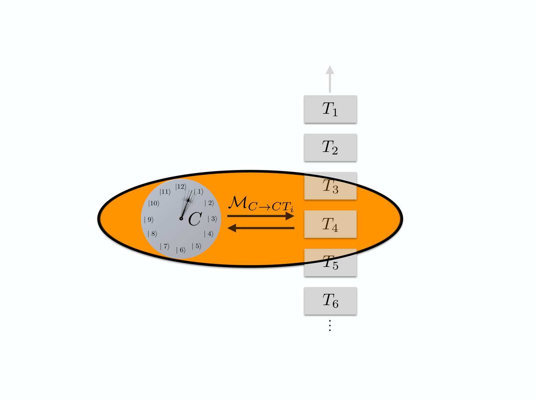
The maps $\mathcal{M}^{\delta}_{C\to C}$ describe the evolution of the state on $C$. But, as argued above, we are generally interested in the information that the clock transmits to the outside. This can be included in our description by virtue of extensions of the maps $\smash{\mathcal{M}^{\delta}_{C\to C}}$. That is, we consider maps $\smash{\mathcal{M}^{\delta}_{C\to CT_{i}}}$ whose target space is a composite system, consisting of $C$ and an additional system $T_{i}$, such that

We call $T_{i}$ tick registers, alluding to the idea that the basic elements of information emitted by a clock are its “ticks”, see Fig 2. Note that while the model of a clock considered here involves an unbounded sequence of finite-dimensional registers that carry the time information it generates, one can show, see [20], that one is able to achieve the precision as reported here for quantum and classical clocks with a single finite register attached to the clock. The model in [20] can achieve this by only utilising a new register state when the clock ticks, in contrast to requiring a new qubit register, $T_{i}$, for every infinitesimal time step. Therefore, its register only needs to be as large as the number of ticks one wishes to record with it. Furthermore, this alternative model has a master equation description for the entire register and clockwork; and hence, contrary to the model considered here, does not require additional degrees of freedom to account for the alignment of the clockwork with a new register $T_{i}$ at every infinitesimal time step.

After these general remarks, we are now ready to state the technical definition. In the following we let all the tick registers $T_{i}$ be isomorphic to a single tick register denoted $T$.

Using Eq. (6), it is easy to see that any family of maps whose reduction to $C$ satisfies Eqs. (4) and (5) also satisfies Eq. (9). The converse is however not necessarily true. Nevertheless, given a family of maps $\{\smash{\mathcal{M}_{C\to CT}^{\delta}}\}_{\delta}$ as in Def. 1, one may always define a family of maps

which meet both Eqs. (4) and (5). In this sense, specifying a map that satisfies Eq. (9) is indeed sufficient to define the continuous and time-independent evolution of a clock. What is more, one may be concerned about technical issues which can arise when dealing with infinite tensor product spaces. Since in any finite time interval, the clock can only tick finitely many times, at any given moment, the state of the register is a classical ensemble of states, each of which contains infinitely many registers $T_{i}$ in the “no-tick” state, and only finitely many in the “tick” state. Thus the resulting infinite dimensional tensor product space is well-defined in our case; see Sec. 2.5. of [21].

The definition does not yet impose any constraints on the tick register, $T$. Since we want to compare different clocks, it will however be convenient to assume that $T$ contains two designated orthogonal states, $\ket{1}$ and $\ket{0}$, which we interpret as “tick” and “no tick”, respectively. The idea is that ticks are the most basic units of time information that a clock can emit. Roughly speaking, a tick indicates that a certain time interval has passed since the last tick.

To know if the clock has ticked after the application of the map $\mathcal{M}^{\delta}_{C\to CT}$, one has to measure the tick register in the “tick” basis $\{\ket{0},\ket{1}\}$. In general, this represents an additional map on the clockwork and register, as Def. 1 allows for the tick register to be coherent in the tick basis, and even entangled with the clockwork system $C$. However, in this work we are only concerned with the probability distribution of ticks (as we characterise the performance of the clock from this alone), and so we incorporate the additional measurement into the map $\mathcal{M}^{\delta}_{C\to CT}$ itself. This is equivalent to requiring the map to restrict the state of the clockwork and tick register to be block-diagonal states in the basis $\{\ket{0},\ket{1}\}$.

Furthermore we consider the behaviour of the tick register in the limit $\delta\to 0$. In principle, the probability of a tick in this limit need not be zero. However, such a clock would correspond to one that has a probability of ticking on every application of the map $\mathcal{M}^{\delta}_{C\to CT}$ independently of the state of the clockwork system, and thus does not provide any information about time.⁵⁵ 5 More precisely, we could express such a clock via the convex combination of two maps, one that does have a zero tick probability for $\delta\to 0$, and one that does not. The second one would provide no time information, and thus only worsen the performance of the clock.

Following the above considerations, we continue with clocks whose maps $\mathcal{M}_{C\to CT}^{\delta}$ provide states on $CT$ that are diagonal in the tick basis $\{\ket{0},\ket{1}\}$, and also satisfy the limit

One may feel inclined to think of a clock whose “ticks” convey additional information, such as the number of previous ticks produced by the clock. For example, often a church bell will produce different chimes to specify the passing of different hours. To treat this within our model, one may think of a (classical) counter, which merely counts the number of tick registers in the state $\ket{1}$. This way, if a tick occurs, one can read the counter and discern the time. Clearly the counter does not need any additional timing devices to function. Importantly, since such a counter only interacts with the tick registers and not the clockwork, it does not directly affect the evolution of the clockwork system $C$.

This concludes our discussion of the generic model of clocks. Real life clocks may also be subject to additional constraints, such as unavoidable de-coherence or power constraints [22],[10]. Since we are considering finite dimensional maps from the clockwork to itself which are continuous, this naturally leads to a finite power consumption, and de-coherence is addressed later with our classical clock case. We furthermore comment on aspects of the clock model in the conclusions, Section V.

As explained above, the specification of the individual maps of the family $\{\mathcal{M}^{\delta}_{C\to CT}\}_{\delta}$ is redundant. The following lemma, which is basically a variant of the Lindblad representation theorem [23], asserts that the family can equivalently be specified in terms of generators.

The proof of this Lemma, which is provided in Appendix A.1, follows the description in Section 3.5.2 of [24]. We call $\rho^{0}_{C}$ the initial state of the clockwork. Furthermore, the operators $J_{j}$ are called tick generators.⁶⁶ 6 While Eq. 12 does not define a dynamical semigroup $CT\rightarrow CT$, it is possible to do so, see supplemental, Sec. A.2.

In addition to determining when the clock ticks, the tick generators $J_{j}$ also define the clockwork’s state after a tick. Clocks for which this state coincides with the initial state $\rho^{0}_{C}$ are of special interest, for they have a particularly appealing mathematical structure and are optimal in terms of their precision in the case of classical clocks.

One may also use the Lindbladian generators to describe the evolution of the clockwork system $C$ as continuous, parametrised by a real variable $t$. From Lemma 1, the following differential equation governs the evolution of the clockwork,

For the tick register, one may take the same limit to find the probability density of a tick being recorded, via the probability that the register is in the state $\ket{1}$,

This limit and the sequence of ticks is discussed in more detail in Section II.5.

Furthermore, consider the case of a clock in which one focuses on a single tick, and tracks the state of the clock only up to the first tick. In this case one can remove the “tick” channel $\sum_{j=1}^{m}J_{j}\rho_{C}J_{j}^{\dagger}$ from the Lindbladian of the clock in Eq. (14), as it represents the state of the clockwork after a tick (see Lemma 1). Thus the description of the entire family of tick generators $\{J_{j}\}_{j=1}^{m}$ is redundant. Labelling the state of the clockwork for just a single tick as $\rho_{C}^{(1)}$, its dynamics are given by (taking Eq. (14) with the tick channel removed)

where

is an arbitrary positive operator representing the ticking dynamics of the clockwork. In this case, the probability density of the first tick being recorded is, from Eq. 15,

This proves useful in the case of reset clocks. As we discuss later, the ticks of a reset clock are a sequence of independent and identically distributed random variables, and thus the first tick suffices to characterise such a clock.

When describing a clock, one may want to distinguish between the intrinsic evolution of the state of the clockwork and the mechanism that transfers information about this state to the outside. A rather generic way to do this is to describe the evolution of the clockwork by a Hamiltonian $\hat{H}_{C}$ on the system $C$, and the transfer of information to the outside by a continuous measurement of the system’s state with respect to a fixed basis $\{\ket{t_{i}}\}_{i=0}^{d-1}$, which we will refer to as the time basis. In order to ensure that the measurement does not disturb the clock’s state too much, the coupling between clockwork and measurement mechanism must be weak. We quantify it in the following by assigning a coupling parameter $V_{i}\in{\mathbbm{R}}_{\geq 0}$ to each of the elements $\ket{t_{i}}$ of the time basis and consider a reset clock (Def. 2). We could then define a quantum clock $(\ket{\psi_{0}}\!\!\bra{\psi_{0}},\{\mathcal{M}^{\delta}_{C\to CT}\}_{\delta})$ with initial state $\ket{\psi_{0}}\!\!\bra{\psi_{0}}$ and maps

where $\smash{\hat{M}^{\delta}_{1,j}=\sqrt{2\delta V_{j}}\ket{\psi_{0}}\!\!\bra{t_{j}}}$ and $\smash{\hat{M}^{\delta}_{0}=\sqrt{{\mathbbm{1}}_{C}-2\delta\hat{V}_{C}}}$ with $\hat{V}_{C}=\sum_{i=0}^{d-1}V_{i}\ket{t_{i}}\!\!\bra{t_{i}}.$

For sufficiently small $\delta$, the quantities $\smash{\{\hat{M}^{\delta}_{1,i}{}^{\dagger}\hat{M}^{\delta}_{1,i}\}_{i=0}^{d-1}}$ together with $\hat{M}^{\delta}_{0}{}^{\dagger}\hat{M}^{\delta}_{0}$ form a positive-operator valued measure (POVM), since

As such, one can interpret Eq. (19), in the following light. The initial state of the clockwork $\rho_{C}$ is measured via the POVMs, followed by allowing the clockwork to freely evolve according to its internal Hamiltonian $\smash{\hat{H}_{C}}$ for an infinitesimal time step $\delta$ and repeating the process. In accordance with Eq. (19) one would then associate the outcome “no-tick” with the POVM element $\hat{M}^{\delta}_{0}{}^{\dagger}\hat{M}^{\delta}_{0}$ and the “tick” outcome with the elements $\smash{\{\hat{M}^{\delta}_{1,i}{}^{\dagger}\hat{M}^{\delta}_{1,i}\}_{i=0}^{d-1}}$. Since the POVM defines a measurement with classical outcome, one may regard the tick as a classical value, i.e., the tick register could be assumed to be classical in this case.

Furthermore, by expanding in $\delta$, Eq. (19) can be written in the form

where we have defined $J_{j}=\sqrt{2V_{j}}\ket{\psi_{0}}\!\!\bra{t_{j}}$. With the further identifications $H=\hat{H}_{C}$, and $\{L_{j}\}_{j=1}^{m}$ with the set of zero operators, we see that Eq. (20) is in the form prescribed by Lemma (1). This ensures that the map $\mathcal{M}^{\delta}_{C\to CT}$ is indeed a clock, according to our definition 9. Consequently, it is easily verified that the $J_{j}$ operators satisfy Eq. (13) and the clock is thus a reset clock. It also follows from Section II.2 that in the continuous limit of clocks, the probability of not getting a “tick” in the time interval $[0,t]$ followed by a tick in the interval time $t,t+\delta t$ is

where $\rho^{(1)}_{C}(t)=\ket{\bar{\psi}_{t}}\!\!\bra{\bar{\psi}_{t}}$, with

Classical physics is widely believed to arise from quantum mechanics due to a mechanism called decoherence. It is a naturally occurring process caused by phenomena in which the quantum state becomes incoherent in some preferred basis [25, 26, 27]. Roughly speaking, a classical clock may be regarded as a clock that satisfies Def. 1, but whose state space is restricted to classical states due to decoherence effects which happen on a time-scale much shorter than the times between ticks.

We allow for any preferred basis. Let us denote it by an arbitrary fixed orthonormal basis $\{\ket{c_{k}}\}_{k=0}^{d-1}$, of the Hilbert space $C$ of the clockwork:

Since the dynamics is restricted to a single basis, we only require the vector of diagonal elements in that basis to describe the clock, and we label this by

where $\mathbf{e}_{m}$ represents the basis vector $\ket{c_{m}}_{C}\!\bra{c_{m}}$ and $v_{C,m}=\braket{c_{m}|\rho_{C}|c_{m}}$ are the diagonal elements of the clock in the preferred basis.

With these definitions in hand, we find that the clock generators take on the simple form of stochastic generators, namely:

See Appendix A.3 for a proof of this corollary. Analogous to the quantum case, we see that $\mathcal{T}$ is the classical version of the tick generator.

In the case of quantum clocks, we used the Lindbladian generators rather than the maps to describe the evolution of the clockwork as continuous and parametrised by $t$ (Section II.2). We can do the same for classical clocks, by taking the limit $\delta\rightarrow 0$, as in Eq. 14. However, in the classical case, since the state is always diagonal w.r.t. a fixed orthonormal basis, we only require the dynamics of the vector of diagonal elements, which is seen to be

As in the quantum case, in the continuous limit we replace the register by a probability density of a tick being recorded, Eq. 15, found to be

Furthermore, if one is focused on a single tick, as in Eq. 16, the reduced dynamics of the state of the clock for a single tick, $v_{C}^{(1)}$ is simply

As mentioned in the introduction, we use the regularity of the tick output of a clock as a measure for its precision. We will now introduce definitions that allow us to express this quantity formally in terms of the clock maps.

A clock (Def. 1) after $N$ applications of the map $\mathcal{M}^{\delta}_{C\to CT}$ gives rise to a probability distribution $P_{T_{j}}(t_{N})$ corresponding to the probability that $j-1$ ticks have occurred during the $N-1$ applications of the map, and the $j^{\textup{th}}$ has occurred at the $N^{\textup{th}}$ application of the map. In the limiting case of continuous clocks discussed in Section II.2, the probability $P_{T_{j}}(t_{N})$, converges to a probability density, such that $P_{T_{j}}(t)\delta t$ is the probability that $j-1$ ticks have occurred in the interval $[0,t)$ and the $j^{\textup{th}}$ has occurred during the interval $[t,t+\delta t]$ for infinitesimal $\delta t>0$. Such probability densities are also known as delay functions or waiting times. In particular, we call $P_{T_{j}}(t)$ the delay function associated with the $j^{\text{th}}$ tick.

The expected time $\mu_{j}$ of the $j^{\text{th}}$ tick and its variance $\sigma_{j}^{2}$ are then given by

for any $j\in{\mathbbm{N}}_{>0}$. Based on these quantities, we can now define the clock precisions $R_{j}$. Note that this is different from the single clock precision $R$, which will be defined below for the particular case of reset clocks.

We will use this definition to define a partial ordering of clocks. For any two clocks $A$, and $B$, with clock accuracies $(R_{j}^{A})_{j\in{\mathbbm{N}_{>0}}}$ and $(R_{j}^{B})_{j\in{\mathbbm{N}_{>0}}}$ respectively, we will say that $A$ is more precise than $B$ iff every tick of $A$ is more precise than the corresponding tick of $B$, i.e., iff $R^{A}_{j}>R^{B}_{j}$ $\forall j\in{\mathbbm{N}_{>0}}$. It is this definition that we refer to when we later prove that quantum clocks are more precise than classical ones.

The characterisation of clocks provided by definition 4 has a number of nice properties. Firstly, it is scale invariant, meaning that the values $R_{j}$ are invariant under the mapping $t$ to $t/a$, for constants $a>0$. In other words, it is a measure of the closeness of the tick intervals to each other rather than to an external timescale, and is not affected by whether these ticks took place over a short or long time scale. Physically, this means that for every clock with precisions $(R_{j})_{j\in{\mathbbm{N}}_{>0}}$, and mean tick times $\mu_{1},\mu_{2},\mu_{3},\dots$, there is another clock with the same precision, but with the ticks occurring on average at times $a\mu_{1},a\mu_{2},a\mu_{3},\dots$. The new clock is constructed from the old clock by mapping $t$ to $t/a$, which is equivalent to rescaling the generators $\{L_{j}\}_{j=1}^{m}$, $\{J_{j}\}_{j=1}^{m}$ and the Hamiltonian $H$, introduced in Lemma 1, by constant factors.

Furthermore, we can now appreciate the simplicity of reset clocks (Def. 2). Since every time such a clock produces a tick, it is reset to its initial state, the ticks represent a sequence of independent events, which are identically distributed. It thus follows that the delay function of the $j^{\text{th}}$ tick, $P_{T_{j}}(t)$, is the convolution of the delay function associated with the 1${}^{\text{st}}$ tick $P_{T_{1}}(t)$, with itself $j$ times. This in turn, gives rise to a simple relationship between the precisions $(R_{j})_{j\in{\mathbbm{N}}_{>0}}$ of reset clocks, (see supplemental B.1.1, and Remark 6 for a detailed argument)

and takes on a particularly satisfactory interpretation. Namely, the precision of the 1${}^{\text{st}}$ tick $R_{1}$, is the number of ticks the clock generates (on average), before the next tick has a standard deviation equal to the mean time between ticks, $\mu_{1}$. As such, roughly speaking, the clock’s useful lifetime is $\mu_{1}R_{1}$, beyond which one can no-longer distinguish between subsequent ticks. To compare two reset clocks, it follows that one only needs to compare their $R_{1}$ values. Given the special significance of $R_{1}$, we will sometimes simply refer to it as $R$.

A similar interpretation is also possible for the $R_{j}$ value of later ticks. For the purpose of illustration, suppose that the mean time between ticks, $\mu_{1}$ is one second. Then $R_{60}$ corresponds to the number of minutes (on average) that the clock can generate until the tick corresponding to the next minute has a standard deviation which is equal to one minute. As such, while according to Eq. (31), $R_{60}$ is 60 times larger than $R_{1}$, this is not to say that “the 60${}^{\text{th}}$ tick is more precise than the 1${}^{\text{st}}$ tick.”

The time–energy uncertainty relation,

has been a controversial concept ever since its conception during the early days of quantum theory, with Bohr, Heisenberg, Pauli and Schrödinger giving it different interpretations and meanings. It is no longer so controversial, thanks to works such as [29, 30], which provide clarifying interpretations to the previous literature, and alternative quantifications, such as the Holevo variance; see, e.g. [11]. Often, at the heart of the controversy, was that in quantum mechanics, as explained in the introduction Section I, time was usually associated with a parameter, rather than an operator.

Since in the present context, we do have operators for time, a lot of this controversy can be circumvented. Indeed, Peres introduced a time operator, $\hat{t}_{c}:=\sum_{k=0}^{d-1}(T_{0}/d)k\ket{\theta_{k}}\!\!\bra{\theta_{k}}$, where $T_{0}=2\pi/\omega$ is the period of the clock Hamiltonian $\hat{H}_{C}$ [17]. In [9] it was shown that the standard deviation of the initial clock state Eq. (35) saturates a time-energy uncertainty relation; $\Delta E\Delta t=1/2$,⁹⁹ 9 The saturation of the bound $\Delta E\Delta t=1/2$ by the Quasi-Ideal clock, is up to an additive correction term which decays faster than any polynomial in $d$. where the standard deviations $\Delta t,$ $\Delta E$ are calculated using the operators $\hat{t}_{c}$ and $\hat{H}_{C}$ respectively. One may be inclined to believe that one can increase the precision of the clock, by decreasing $\Delta t$ as a consequence of a larger $\Delta E$. While indeed decreasing $\sigma_{0}$ does have this effect, it would be naive to believe this paints the full picture.

To study this effect as the clock moves around the clock-face, let $\Delta E(t)$ be the standard deviation of the clock coefficients de-phased in the energy basis, $\{\braket{E_{n}|\rho_{C}(t)|E_{n}}\}_{n=0}^{d-1}$. We will define the standard deviation in the time basis similarly, but here one has to be careful since the time basis $\{\ket{\theta_{k}}\}$ has circular boundary conditions, meaning $\ket{\theta_{k}}=\ket{\theta_{k+1\,(\mathrm{mod}\,d)}}$. Consequently, the state will “jump” from the state $\ket{\theta_{d-1}}$ to $\ket{\theta_{0}}$ as it completes one period of its motion. We are not interested in the jumps due to the boundary effects, and therefore will denote $\Delta C(t)$ the standard deviation of the coefficients $\braket{\theta_{k}|\rho_{C}(t)|\theta_{k}}$ with the circular boundary conditions replaced with open boundaries¹⁰¹⁰ 10 When the population $\braket{\theta_{k}|\rho_{C}(t)|\theta_{k}}$ reaches the position $d-1$, rather than subsequently appearing at position $0$, it will be assigned to position $d$, and subsequently to position $d+1$, etc.. This way, we mimic the hands of a real clock, which visually do not suddenly “jump” at 12 O’clock. The quantity $\Delta C(t)$ is plotted for the Quasi-Ideal clock and SWP clocks in Fig. a) 4.

Firstly, if $\sigma_{0}$ is too small, the clock will disperse too much due to its dynamics and time measurements. Secondly, another way to decrease $\Delta t$ and increase $\Delta E$, is via reducing $T_{0}$, yet this has no effect on the precision of the clock. This latter observation is also related to how our measure of precision $R_{1}$, is invariant under a re-scaling of time, as discussed in Section I. In other words, for the lower bound in Eq. 36 to exceed the classically permitted value of $d$, the clock uncertainty in the time basis $\Delta t$, must be smaller than the uncertainty in the energy basis $\Delta E$ during the time in which the clock is running. In Fig. 4 a), the orange plot has $\Delta C(t)\approx\Delta E(t)\approx\sqrt{1/2}$. This is suboptimal, since the POVMs used to measure ticks are diagonal in the time basis $\{\ket{\theta_{k}}\}$. Furthermore, the blue curve has a smaller $\Delta C(t)$, and according to Theorem 2 can achieve $R_{1}>d$. However, if we continue to choose initial clock states with smaller $\Delta C(0)$, we run into a problem, namely in the limit $\sigma_{0}\rightarrow 0^{+}$, we recover the SWP clock state (green), which has a very large $\Delta C(t)$ at later times.

Another interesting aspect regarding time and energy, is what is the internal energy of the clock. We can easily answer this question for the Quasi-Ideal clock. Note that for $n_{0}=(d-1)/2$, the mean energy of the Quasi-Ideal clock is $\omega\,d/2+o\left(d\right)$, thus Theorem 2 implies that high precision can be achieved with a modest linear increase in internal energy.

Metrology is the science of measuring unknown parameters. Here, like in other areas of quantum science, it has been shown that allowing for quantum effects can vastly improve the precision of measurements in comparison with the optimal classical protocols. Quantum metrology is now a mature discipline with a vast literature[31]; and as such, it is appropriate to compare our results about clocks with them.

The basic setup in metrology is as follows. When attempting to measure an unknown parameter in a physical system, we prepare a probe state, let it evolve, and finally measure the evolved system. The evolution stage is according to the unitary operator $U_{x}:=\mathrm{e}^{-\mathrm{i}x\hat{H}}$, where $\hat{H}$ is a known Hamiltonian.

The model of a clock described in this manuscript differs substantially from the metrology setup above. The easiest way to convey the main difference is via a simple example: for the purpose of illustration, imagine you were told to perform a particular task after 5 seconds. If you had a clock you could wait for 5 ticks to pass according to it, and perform your designated task. However, in the case of the metrology set-up one can only estimate the time when one happened to measure the probe. As discussed in Section I, this marks an important division between time keeping devices, and those based on the standard metrology set-ups described here, fall into the category of stopwatches and not clocks, according to our definitions. One could of course use a very precise stopwatch in combination with a not so precise clock, by measuring the stopwatch when the clock ticks, and resetting the stopwatch immediately after measuring it. While one would know to high precision when in time these ticks occurred, their distribution in time would still be the same as if we did not have access to the stopwatch. As such, one can observe that even this combination cannot be substituted for a more precise clock.

The quantum speed limit, $\tau_{\textup{QSL}}$ is the minimum time $t_{\textup{QSL}}$ required for a state $\ket{\psi(0)}$ to become orthogonal to itself, $\braket{\psi(0)|\psi(t_{\textup{QSL}})}=0$ under unitary time evolution, $\ket{\psi(t)}=\mathrm{e}^{-\mathrm{i}t\hat{H}}$. The celebrated Margolus-Levitin and Mandelstam-Tamm bounds, impose a tight lower limit in terms of the mean and standard deviation of $\hat{H}$ w.r.t. the initial state $\ket{\psi(0)}$ [32]. It has found many applications in the field of thermodynamics, metrology, and the study of the rate at which information can be transmitted from a quantum system an external observer [33, 34].

One may also be inclined to think that the fundamental limitations on the precision of clocks is related to how quickly the initial clock state becomes perfectly distinguishable to itself, when measured by an external observer. Indeed, the quicker states become distinguishable, the faster one can extract timing information from the clock state. Unfortunately, a simple example will reveal how the situation of a clock is too subtle to be captured by such simple arguments. The quantum speed limit $t_{\textup{QSL}}$ of the SWP clock is precisely $T_{0}/d=2\pi/(\omega d)$, since the states satisfy $\mathrm{e}^{-\mathrm{i}\hat{H}_{C}T_{0}/d}\ket{\theta_{k}}=\ket{\theta_{k+1}}$. On the other hand, the Quasi-Ideal clock has a quantum speed limit of much larger than $T_{0}$. Yet, as described in Fig. 4 b), numerics predict that while the SWP clock has a higher precision than the optimal classical clock, it is less precise than the Quasi-Ideal clock. The explanation of this is that, contrary to the Quasi-Ideal clock, the SWP clock — at the expense of a shorter quantum speed limit time — becomes highly spread-out in the time basis for times in-between becoming orthogonal to itself; thus incurring large $\Delta C(t)$ during these times [see green plot in Fig. 4 a)]. In summery, the quantum speed limit only tells us about how long it takes for a clock state to become distinguishable to itself, but fails to quantify the behaviour in-between. Since a clock has to produce a continuous stream of “tick”, “no-tick” information, the nature of dynamics of the clock at all times is of high importance.

All authors contributed to the ideas and results within this work. M.W. proved the lower bound for quantum clocks (Theorem 2). R.S. proved the upper bound on classical clocks (Theorem 1). S.S. provided numerics on quantum clocks (Fig. 4). M.W. and R.R. wrote the main text.

References

- [1] Andrew D. Ludlow, Martin M. Boyd, Jun Ye, E. Peik, and P. O. Schmidt. Optical atomic clocks. Rev. Mod. Phys., 87:637–701, Jun 2015.
- [2] Jonathan P. Dowling and Gerard J. Milburn. Quantum technology: the second quantum revolution. Philos. Trans. Royal Soc. A, 361(1809):1655–1674, 2003.
- [3] Wolfgang Pauli. Handbuch der Physik. Springer, Berlin, 24:83—272, 1933.
- [4] Wolfgang Pauli. Encyclopedia of Physics. Springer, Berlin, 1:60, 1958.
- [5] Wolfgang Pauli. General principles of quantum mechanics. Springer Science & Business Media, 2012.
- [6] A.S. Holevo. Probabilistic and Statistical Aspects of Quantum Theory. Publications of the Scuola Normale Superiore. Scuola Normale Superiore, 2011.
- [7] Sandra Ranković, Yeong-Cherng Liang, and Renato Renner. Quantum clocks and their synchronisation - the Alternate Ticks Game. arXiv:1506.01373, 2015.
- [8] Christopher A. Fuchs and Asher Peres. Quantum-state disturbance versus information gain: Uncertainty relations for quantum information. Phys. Rev. A, 53:2038–2045, Apr 1996.
- [9] Mischa P. Woods, Ralph Silva, and Jonathan Oppenheim. Autonomous Quantum Machines and Finite-Sized Clocks. Annales Henri Poincaré, Oct 2018.
- [10] Paul Erker, Mark T. Mitchison, Ralph Silva, Mischa P. Woods, Nicolas Brunner, and Marcus Huber. Autonomous quantum clocks: Does thermodynamics limit our ability to measure time? Phys. Rev. X, 7:031022, Aug 2017.
- [11] Vladimir Bužek, Radoslav Derka, and Serge Massar. Optimal quantum clocks. Phys. Rev. Lett., 82:2207–2210, Mar 1999.
- [12] Helmut Salecker and Eugene P. Wigner. Quantum limitations of the measurement of space-time distances. Phys. Rev., 109:571–577, Jan 1958.
- [13] Gonzalo Muga, Rafael Sala Mayato, and Ínigo Egusquiza, editors. Time in Quantum Mechanics Vol 1. Lecture Notes in Physics. Springer Berlin Heidelberg, 2007.
- [14] Gonzalo Muga, Andreas Ruschhaupt, and Adolfo del Campo, editors. Time in Quantum Mechanics Vol 2. Lecture Notes in Physics. Springer Berlin Heidelberg, 2010.
- [15] Sandra Stupar, Christian Klumpp, Nicolas Gisin, and Renato Renner. Performance of Stochastic Clocks in the Alternate Ticks Game. 2018. ArXiv:1806.08812.
- [16] Thomas Pashby. Time and the foundations of quantum mechanics. PhD thesis, University of Pittsburgh, 2014.
- [17] Asher Peres. Measurement of time by quantum clocks. American Journal of Physics, 48(7):552–557, 1980.
- [18] David Gross, Vincent Nesme, Holger Vogts, and Reinhard. F. Werner. Index theory of one dimensional quantum walks and cellular automata. Communications in Mathematical Physics, 310(2):419–454, Mar 2012.
- [19] Paul Busch, Marian Grabowski, and Pekka J. Lahti. Time observables in quantum theory. Physics Letters A, 191(5):357 – 361, 1994.
- [20] Mischa P. Woods. Autonomous Ticking Clocks from Axiomatic Principles. Quantum, 5:381, January 2021.
- [21] N. Weaver. Mathematical Quantization. Studies in Advanced Mathematics. CRC Press, 2001.
- [22] Paul Erker. The Quantum Hourglass. 2014. ETH Zürich.
- [23] Göran Lindblad. On the generators of quantum dynamical semigroups. Commun. Math. Phys., 48(2):119–130, Jun 1976.
- [24] John Preskill. Chapter 3. Foundations of Quantum Theory II: Measurement and Evolution. July 2015. Lecture notes available.
- [25] Maximilian A. Schlosshauer. Decoherence: and the Quantum-To-Classical Transition. The Frontiers Collection. Springer Berlin Heidelberg, 2007.
- [26] Igor Pikovski, Magdalena Zych, Fabio Costa, and Časlav Brukner. Universal decoherence due to gravitational time dilation. Nature Physics, 11:668, 2015.
- [27] Wojciech Zurek. Quantum Darwinism. Nature Physics, 5, 2009.
- [28] Yuxiang Yang and Renato Renner. Ultimate limit on time signal generation, Apr 2020. arXiv:2004.07857.
- [29] Paul Busch. The Time–Energy Uncertainty Relation, pages 73–105. Springer Berlin Heidelberg, Berlin, Heidelberg, 2008.
- [30] Yakir Aharonov, Serge Massar, and Sandu Popescu. Measuring energy, estimating hamiltonians, and the time-energy uncertainty relation. Phys. Rev. A, 66:052107, Nov 2002.
- [31] Vittorio Giovannetti, Seth Lloyd, and Lorenzo Maccone. Advances in quantum metrology. Nature Photonics, 5(4):222–229, Apr 2011.
- [32] Sebastian Deffner and Steve Campbell. Quantum speed limits: from heisenberg’s uncertainty principle to optimal quantum control. J. Phys. A, 50(45):453001, 2017.
- [33] Jacob D. Bekenstein. Generalized second law of thermodynamics in black-hole physics. Phys. Rev. D, 9:3292–3300, Jun 1974.
- [34] Jacob D. Bekenstein and Marcelo Schiffer. Quantum limitations on the storage and transmission of information. Int. J. Mod. Phys. C, 01(04):355–422, 1990.
- [35] E. Oelker, R. B. Hutson, C. J. Kennedy, L. Sonderhouse, T. Bothwell, A. Goban, D. Kedar, C. Sanner, J. M. Robinson, G. E. Marti, D. G. Matei, T. Legero, M. Giunta, R. Holzwarth, F. Riehle, U. Sterr, and J. Ye. Demonstration of 4.8 stability at 1 s for two independent optical clocks. Nature Photonics, 13(10):714–719, 2019.
- [36] Shishir Khandelwal, Maximilian P.E. Lock, and Mischa P. Woods. Universal quantum modifications to general relativistic time dilation in delocalised clocks. Quantum, 4:309, August 2020.
- [37] Charis Anastopoulos and Bei Lok Hu. Equivalence principle for quantum systems: dephasing and phase shift of free-falling particles. Classical and Quantum Gravity, 35(3):035011, Jan 2018.
- [38] Magdalena Zych, Fabio Costa, Igor Pikovski, and Časlav Brukner. Quantum interferometric visibility as a witness of general relativistic proper time. Nat. Commun., 2:505, 2011.
- [39] Costantino Budroni, Giuseppe Vitagliano, and Mischa P. Woods. Ticking-clock performance enhanced by nonclassical temporal correlations. Phys. Rev. Research, 3:033051, Jul 2021.
- [40] Andrzej Kossakowski. On quantum statistical mechanics of non-Hamiltonian systems. Rep. Math. Phys., 3:247—274, 1972.
- [41] Gilles Pütz et al. In preparation, 2019.
- [42] Athanasios Papoulis and S. Unnikrishna Pillai. Probability, random variables, and stochastic processes. Boston: McGraw-Hill, 2002.
- [43] Walter Rudin. Principles of Mathematical Analysis. International series in pure and applied mathematics. McGraw-Hill, 1976.
- [44] Andrey Kolmogoroff. Über die analytischen methoden in der wahrscheinlichkeitsrechnung. Mathematische Annalen, 104(1):415–458, Dec 1931.
- [45] Rajendra Bhatia. Matrix analysis. Graduate Texts in Mathematics, 169. Springer-Verlag, New York, 1997.
Appendices and Table of Contents
Appendix A Modelling of Clocks
A.1 Proof of Lemma 1
See 1
Proof.
Consider an operator-sum representation of the map , i.e.,