跳到论文正文
W Papers独立论文阅读器 arXiv:1806.00477 论文正文 计算阅读时间 · 0%
引用这篇论文根据当前论文元数据生成,正式投稿前建议核对。


License: arXiv.org perpetual non-exclusive license
arXiv:1806.00477v1 [math.NA] 31 May 2018

Fractional Sensitivity Equation Method:
Applications to Fractional Model Construction Thanks: This work was supported by the AFOSR Young Investigator Program (YIP) award (FA9550-17-1-0150).

Ehsan Kharazmi Note: Department of Computational Mathematics, Science, and, Engineering & Department of Mechanical Engineering, Michigan State University, 428 S Shaw Lane, East Lansing, MI 48824, USA    Mohsen Zayernouri Note: Department of Computational Mathematics, Science, and, Engineering & Department of Mechanical Engineering, Michigan State University, 428 S Shaw Lane, East Lansing, MI 48824, USA, Corresponding author; zayern@msu.edu
Abstract

Fractional differential equations provide a tractable mathematical framework to describe anomalous behavior in complex physical systems, yet they introduce new sensitive model parameters, i.e. derivative orders, in addition to model coefficients. We formulate a sensitivity analysis of fractional models by developing a fractional sensitivity equation method. We obtain the adjoint fractional sensitivity equations, in which we present a fractional operator associated with logarithmic-power law kernel. We further construct a gradient-based optimization algorithm to compute an accurate parameter estimation in fractional model construction. We develop a fast, stable, and convergent Petrov-Galerkin spectral method to numerically solve the coupled system of original fractional model and its corresponding adjoint fractional sensitivity equations.

keywords
sensitive fractional orders, model error, logarithmic-power law kernel, Petrov-Galerkin spectral method, iterative algorithm, parameter estimation.

1 Introduction

The experimental observations in a divers number of complex physical systems reveal ubiquitous anomalous behavior in the associated underlying processes [62, 61], where the anomaly manifests itself in skewness and sharpness of heavy tailed distributions. Fractional differential equations, which generalize their integer order counterparts, construct a rigorous mathematical framework to formulate models that flawlessly describe such anomalies. The excellence of fractional operator in accurate prediction of non-locality and memory effects is the inherent non-local nature of singular power-law kernel, whose order is defined as fractional derivative order, i.e. fractional index. Theses operators are being extensively used in analysis and design of models for a wide range of multi-scale multi-physics phenomena. Examples include viscoelastic materials and wave propagation [39, 55, 41], non-Brownian transport phenomena in porous media and disordered materials [6, 41], non-Newtonian complex fluids with multi-phase applications and rheology [23, 52, 24, 16, 22], multi-scale patterns in biological tissue [43, 44, 38, 4, 17], chaos/fractals and automatic control [31, 18]. However, the key challenges of such models are the excessive computational cost in numerically integrating the convolution operation, and more importantly, introducing fractional derivative orders as extra model parameters, whose values are essentially obtained from experimental data. The sensitivity assessment of fractional models with respect to fractional indecis can build a bridge between experiments and mathematical models to gear observable data via proper optimization techniques, and thus, systematically improve the existing models in both analysis and design approaches. We formulate a mathematical framework by developing a fractional sensitivity equation method, where we investigate the response sensitivity of fractional differential equations with respect to model parameters including derivative orders, and further construct an iterative algorithm in order to exploit the obtained sensitivity field in parameter estimation.

Fractional Sensitivity Analysis. Sensitivity assessment approaches are commonly categorized as, finite difference, continuum and discrete derivatives, and computational or automatic differentiation, where the sensitivity coefficients are generally defined as partial derivative of corresponding functions (model output) with respect to design/analysis parameters of interest. Finite difference schemes use a first order Taylor series expansion to approximate the sensitivity coefficients, where accuracy depends strongly on step increment [40, 51]. Continuum and discrete derivative techniques however, differentiate the system response with respect to parameters, where the former, which is also known as sensitivity equation method (SEM, see [37, 72] and references therein), directly computes the derivatives and obtain a set of (coupled) adjoint continuum sensitivity equations; while the latter performs differentiation after discretization of original equation [53]. Automatic differentiation method also refers to a differentiation of the computer code [8, 10, 9]. Fig.2 in [56] provides a descriptive schematic of these different approaches. We extend the continuum derivative technique to develop a fractional sensitivity equation method (FSEM) in the context of fractional partial differential equations (FPDEs). To formulate the sensitivity analysis framework, we let qq be a set of model parameters including fractional indices and obtain the adjoint fractional sensitivity equations (FSEs) by taking the partial derivative of FPDE with respect to qq. These adjoint equations introduce a new fractional operator, associated with the logarithmic-power law kernel, which to best of our knowledge has been presented for the first time here in the context of fractional sensitivity analysis. The key property of derived FSEs is that they preserve the structure of original FPDE. Thus, similar discretization scheme and forward solver can be readily applied with a minimal required changes.

Model Construction: Estimation of Fractional Indices. Several numerical methods have been developed to solve inverse problem of model construction from available experimental observations or synthetic data. They typically convert the problem of model parameter estimation into an optimization problem, and then, formulate a suitable estimator by minimizing an objective function. These methods are stretched over but no limited to perturbation methods [60], weighted least squares approach [12, 15, 25], nonlinear regression [34], and Levenberg-Marquardt method [20, 13, 63, 64]. We develop a bi-level FSEM-based parameter estimation method in order to construct fractional models, in a sense that the method obtains model coefficients in one level, and then searches for estimate of fractional indices in the next level. We formulate the optimization problem by defining objective functions as two types of model error that measures the difference in computed output/input of fractional model with true output/input in an L2L^{2}-norm sense. We further formulate a gradient-based minimizer, employing developed FSEM, and propose a two-stage search algorithm, namely, coarse grid searching and nearby solution. The first stage construct a crude manifold of model error over a coarse discretization of parameter space to locate a local neighborhood of minimum, and the second stage uses the gradient decent method in order to converge to the minimum point.

Discretization Scheme. The iterative nature of parameter estimators instruct simulation of fractional model at each iteration step of model parameters. Therefore, one of the major tasks in computational model construction is to develop numerical methods that can efficiently discretize the physical domain and accurately solve the fractional model. The sensitivity framework additionally raise the complication by rendering coupled systems of FPDE and adjoint FSEs, and thus, demanding more versatile schemes. In addition to numerous finite difference methods [21, 54, 35, 57, 59, 11, 73, 71], recent works have elaborated efficient spectral schemes, for discretizing FPDEs in physical domain, see e.g., [46, 35, 26, 27, 32, 33, 14, 58, 7]. More recently, Zayernouri et al. [68, 66] developed two new spectral theories on fractional and tempered fractional Sturm-Liouville problems, and introduced explicit corresponding eigenfunctions, namely Jacobi poly-fractonomials of first and second kind. These eignefunctions are comprised of smooth and fractional parts, where the latter can be tunned to capture singularities of true solution. They are successfully employed in constructing discrete solution/test function spaces and developing a series of high-order and efficient Petrov-Galerkin spectral methods, see [70, 67, 69, 55, 49, 47, 30, 29, 28, 36, 50, 48]. We formulate a numerical scheme in solving coupled system of FPDE and adjoint FSEs by extending the mathematical framework in [49] and accommodating extra required regularity in the underlying function spaces. We employ Jacobi poly-fractonomials and Legendre polynomials as temporal and spatial basis/test functions, respectively, to develop a Petrov-Galerkin (PG) spectral method. The smart choice of coefficients in spatial basis/test functions yields symmetric property in the resulting mass/stiffness matrices, which is then exploited to formulate a fast solver. Following similar procedure as in [49], we also show that the coupled system is mathematically well-posed, and the proposed numerical scheme is stable.

The rest of paper is organized as follows. In section 2, we recall some preliminary definitions in fractional calculus and define proper solution/test spaces beside useful lemmas. In section 3, we define the problem by providing the fractional model, and then take the weak form of the problem as well. We develop FSEM in section 4 for the case of FIVP and FPDE. We define the underlying mathematical frame work for the coupled system of FPDE and FSEs and also construct our Petrov-Galerkin spectral numerical scheme. Moreover, we develop the FSEM based model construction algorithm in section 5 and finally, provide the numerical results in section 6. We conclude the paper with a summary and conclusion.

2 Definitions

Let ξ∈[−1,1]\xi\in[-1,1]. The left- and right-sided fractional derivative of order σ\sigma, n−1<σ≤nn-1<\sigma\leq n, n∈ℕn\in\mathbb{N}, are defined as (see e.g., [42, 45])

(𝒟ξσ−1R​L)​u​(ξ)=1Γ⁡(n−σ)​dnd​ξn​∫−1ξu⁡(s)​d​s(ξ−s)σ+1−n,ξ>−1,\displaystyle(\prescript{RL}{-1}{\mathcal{D}}_{\xi}^{\sigma})u(\xi)=\frac{1}{\Gamma(n-\sigma)}\frac{d^{n}}{d\xi^{n}}\int_{-1}^{\xi}\frac{u(s)ds}{(\xi-s)^{\sigma+1-n}},\quad\xi>-1, (2.1)
(𝒟1σξR​L)​u​(ξ)=1Γ⁡(n−σ)​(−d)nd​ξn​∫ξ1u⁡(s)​d​s(s−ξ)σ+1−n,ξ<1,\displaystyle(\prescript{RL}{\xi}{\mathcal{D}}_{1}^{\sigma})u(\xi)=\frac{1}{\Gamma(n-\sigma)}\frac{(-d)^{n}}{d\xi^{n}}\int_{\xi}^{1}\frac{u(s)ds}{(s-\xi)^{\sigma+1-n}},\quad\xi<1, (2.2)

respectively. An alternative approach in defining the fractional derivatives is the left- and right-sided Caputo derivatives of order σ\sigma, defined, as

(𝒟ξσ−1C​u)​(ξ)=1Γ⁡(n−σ)​∫−1ξu(n)​(s)​d​s(ξ−s)σ+1−n,ξ>−1,\displaystyle(\prescript{C}{-1}{\mathcal{D}}_{\xi}^{\sigma}u)(\xi)=\frac{1}{\Gamma(n-\sigma)}\int_{-1}^{\xi}\frac{u^{(n)}(s)ds}{(\xi-s)^{\sigma+1-n}},\quad\xi>-1, (2.3)
(𝒟1σξC​u)​(ξ)=1Γ⁡(n−σ)​∫ξ1u(n)​(s)​d​s(s−ξ)σ+1−n,ξ<1.\displaystyle(\prescript{C}{\xi}{\mathcal{D}}_{1}^{\sigma}u)(\xi)=\frac{1}{\Gamma(n-\sigma)}\int_{\xi}^{1}\frac{u^{(n)}(s)ds}{(s-\xi)^{\sigma+1-n}},\quad\xi<1. (2.4)

By performing an affine mapping from the standard domain [−1,1][-1,1] to the interval t∈[a,b]t\in[a,b], we obtain

𝒟tσaR​L​u\displaystyle\prescript{RL}{a}{\mathcal{D}}_{t}^{\sigma}u =\displaystyle= (2b−a)σ​(𝒟ξσ−1R​L​u)​(ξ),\displaystyle(\frac{2}{b-a})^{\sigma}(\prescript{RL}{-1}{\mathcal{D}}_{\xi}^{\sigma}\,u)(\xi), (2.5)
𝒟tσaC​u\displaystyle\prescript{C}{a}{\mathcal{D}}_{t}^{\sigma}u =\displaystyle= (2b−a)σ​(𝒟ξσ−1C​u)​(ξ).\displaystyle(\frac{2}{b-a})^{\sigma}(\prescript{C}{-1}{\mathcal{D}}_{\xi}^{\sigma}\,u)(\xi). (2.6)

Hence, we can perform the operations in the standard domain only once for any given σ\sigma and efficiently utilize them on any arbitrary interval without resorting to repeating the calculations. Moreover, the corresponding relationship between the Riemann-Liouville and Caputo fractional derivatives in [a,b][a,b] for any σ∈(0,1)\sigma\in(0,1) is given by

(𝒟tσaR​L​u)​(t)=u⁡(a)Γ⁡(1−σ)​(t−a)σ+(𝒟tσaC​u)​(t).(\prescript{RL}{a}{\mathcal{D}}_{t}^{\sigma}\,u)(t)=\frac{u(a)}{\Gamma(1-\sigma)(t-a)^{\sigma}}+(\prescript{C}{a}{\mathcal{D}}_{t}^{\sigma}\,u)(t). (2.7)
Definition 2.1.

We define the following left- and right-sided integro-differential operator with logarithmic-power law kernel, namely Log-Pow integro-differential operator, given as,

𝒟xσaR​L−L​P​u​(x)=1Γ⁡(n−σ)​dnd​xn​∫axlog⁡(x−s)​u​(s)(x−s)σ−n+1​𝑑s,\displaystyle\prescript{RL-LP}{a}{\mathcal{D}}_{x}^{\sigma}u(x)=\frac{1}{\Gamma(n-\sigma)}\frac{d^{n}}{dx^{n}}\int_{a}^{x}\frac{\log(x-s)\,u(s)}{(x-s)^{\sigma-n+1}}ds, (2.8)
𝒟bσxR​L−L​P​u​(x)=1Γ⁡(n−σ)​(−d)nd​xn​∫xblog⁡(s−x)​u​(s)(s−x)σ−n+1​𝑑s,\displaystyle\prescript{RL-LP}{x}{\mathcal{D}}_{b}^{\sigma}u(x)=\frac{1}{\Gamma(n-\sigma)}\frac{(-d)^{n}}{dx^{n}}\int_{x}^{b}\frac{\log(s-x)\,u(s)}{(s-x)^{\sigma-n+1}}ds, (2.9)
𝒟xσaC−L​P​u​(x)=1Γ⁡(n−σ)​∫axlog⁡(x−s)​u(n)​(s)(x−s)σ−n+1​𝑑s,\displaystyle\prescript{C-LP}{a}{\mathcal{D}}_{x}^{\sigma}u(x)=\frac{1}{\Gamma(n-\sigma)}\,\int_{a}^{x}\frac{\log(x-s)\,u^{(n)}(s)}{(x-s)^{\sigma-n+1}}ds, (2.10)
𝒟bσxC−L​P​u​(x)=1Γ⁡(n−σ)​∫xblog⁡(s−x)​u(n)​(s)(s−x)σ−n+1​𝑑s,\displaystyle\prescript{C-LP}{x}{\mathcal{D}}_{b}^{\sigma}u(x)=\frac{1}{\Gamma(n-\sigma)}\,\int_{x}^{b}\frac{\log(s-x)\,u^{(n)}(s)}{(s-x)^{\sigma-n+1}}ds, (2.11)

where R​L−L​PRL-LP and C−L​PC-LP stand for Log-Pow integro-differential operator, which partially resemble the fractional derivative in Riemann-Liouville and Caputo sense, respectively. The following lemma shows a useful relation between the two aforementioned operators.

Lemma 2.2.

Let x∈[a,b]x\in[a,b]. Then, the following relation holds.

Part A: σ∈(0,1)\sigma\in(0,1)

𝒟xσaR​L−L​P​u​(x)=u⁡(a)Γ⁡(1−σ)​log⁡(x−a)(x−a)σ+𝒟xσaC−L​P​u​(x).\displaystyle\prescript{RL-LP}{a}{\mathcal{D}}_{x}^{\sigma}\,u(x)=\frac{u(a)}{\Gamma(1-\sigma)}\frac{\log(x-a)}{(x-a)^{\sigma}}+\prescript{C-LP}{a}{\mathcal{D}}_{x}^{\sigma}\,u(x). (2.12)

Part B: σ∈(1,2)\sigma\in(1,2)

𝒟xσaR​L−L​P​u​(x)=u⁡(a)Γ⁡(2−σ)​1+(1−σ)​log⁡(x−a)(x−a)σ+u′​(a)Γ⁡(2−σ)​log⁡(x−a)(x−a)σ−1+𝒟xσaC−L​P​u​(x).\displaystyle\prescript{RL-LP}{a}{\mathcal{D}}_{x}^{\sigma}\,u(x)=\frac{u(a)}{\Gamma(2-\sigma)}\frac{1+(1-\sigma)\log(x-a)}{(x-a)^{\sigma}}+\frac{u^{\prime}(a)}{\Gamma(2-\sigma)}\frac{\log(x-a)}{(x-a)^{\sigma-1}}+\prescript{C-LP}{a}{\mathcal{D}}_{x}^{\sigma}\,u(x). (2.13)

Proof.

See Appendix A for proof.

2.1 Fractional Sobolev Spaces

We define some functional spaces and their associated norms [30, 32]. By Hσ(ℝ)={u(t)|u∈L2(ℝ);(1+|ω|2)σ2F(u)(ω)∈L2(ℝ)}H^{\sigma}(\mathbb{R})=\big\{u(t)|u\in L^{2}(\mathbb{R});\,(1+|\omega|^{2})^{\frac{\sigma}{2}}F(u)(\omega)\in L^{2}(\mathbb{R})\big\}, σ≥0\sigma\geq 0, we denote the fractional Sobolev space on ℝ\mathbb{R}, endowed with norm ‖u‖Hℝσ=‖(1+|ω|2)σ2​F​(u)​(ω)‖L2​(ℝ)\|u\|_{H^{\sigma}_{\mathbb{R}}}=\|(1+|\omega|^{2})^{\frac{\sigma}{2}}F(u)(\omega)\|_{L^{2}(\mathbb{R})}, where ℱ⁡(u)\mathcal{F}(u) represents the Fourier transform of uu. Subsequently, we denote by Hσ(Λ)={u∈L2(Λ)|∃u~∈Hσ(ℝ)s.t.u~|Λ=u}H^{\sigma}(\Lambda)=\big\{u\in L^{2}(\Lambda)\,|\,\exists\tilde{u}\in H^{\sigma}(\mathbb{R})\,\,s.t.\,\,\tilde{u}|_{\Lambda}=u\big\}, σ≥0\sigma\geq 0, the fractional Sobolev space on any finite closed interval, e.g. Λ=(a,b)\Lambda=(a,b), with norm ‖u‖Hσ​(Λ)=infu~∈Hℝσ,u~|Λ=u​‖u~‖Hσ​(ℝ)\|u\|_{H^{\sigma}(\Lambda)}=\underset{\tilde{u}\in H^{\sigma}_{\mathbb{R}},\,\tilde{u}|_{\Lambda}=u}{\inf}\,\|\tilde{u}\|_{{}H^{\sigma}(\mathbb{R})}. We define the following useful norms as:

∥⋅∥Hσl​(Λ)=(∥𝒟xσa(⋅)∥L2​(Λ)2+∥⋅∥L2​(Λ)2)12,\displaystyle\|\cdot\|_{{{}^{l}}H^{\sigma}(\Lambda)}=\Big(\|\prescript{}{a}{\mathcal{D}}_{x}^{\sigma}\,(\cdot)\|_{L^{2}(\Lambda)}^{2}+\|\cdot\|_{L^{2}(\Lambda)}^{2}\Big)^{\frac{1}{2}},
∥⋅∥Hσr​(Λ)=(∥𝒟bσx(⋅)∥L2​(Λ)2+∥⋅∥L2​(Λ)2)12,\displaystyle\|\cdot\|_{{{}^{r}}H^{\sigma}(\Lambda)}=\Big(\|\prescript{}{x}{\mathcal{D}}_{b}^{\sigma}\,(\cdot)\|_{L^{2}(\Lambda)}^{2}+\|\cdot\|_{L^{2}(\Lambda)}^{2}\Big)^{\frac{1}{2}},
∥⋅∥Hσc​(Λ)=(∥𝒟bσx(⋅)∥L2​(Λ)2+∥𝒟xσa(⋅)∥L2​(Λ)2+∥⋅∥L2​(Λ)2)12,\displaystyle\|\cdot\|_{{{}^{c}}H^{\sigma}(\Lambda)}=\Big(\|\prescript{}{x}{\mathcal{D}}_{b}^{\sigma}\,(\cdot)\|_{L^{2}(\Lambda)}^{2}+\|\prescript{}{a}{\mathcal{D}}_{x}^{\sigma}\,(\cdot)\|_{L^{2}(\Lambda)}^{2}+\|\cdot\|_{L^{2}(\Lambda)}^{2}\Big)^{\frac{1}{2}},

where the equivalence of ∥⋅∥Hσl​(Λ)\|\cdot\|_{{{}^{l}}H^{\sigma}(\Lambda)} and ∥⋅∥Hσr​(Λ)\|\cdot\|_{{{}^{r}}H^{\sigma}(\Lambda)} are shown in [32, 19, 33]. We show the equivalence of these two norms with ∥⋅∥Hσc​(Λ)\|\cdot\|_{{{}^{c}}H^{\sigma}(\Lambda)} in the following lemma.

Lemma 2.3.

Let σ≥0\sigma\geq 0 and σ≠n−12\sigma\neq n-\frac{1}{2}. Then, the norms ∥⋅∥Hσl​(Λ)\|\cdot\|_{{{}^{l}}H^{\sigma}(\Lambda)} and ∥⋅∥Hσr​(Λ)\|\cdot\|_{{{}^{r}}H^{\sigma}(\Lambda)} are equivalent to ∥⋅∥Hσc​(Λ)\|\cdot\|_{{{}^{c}}H^{\sigma}(\Lambda)}.

Proof.

See Appendix B for proof.

We also define C0∞​(Λ)C^{\infty}_{0}(\Lambda) as the space of smooth functions with compact support in (a,b)(a,b). We denote by H0σl​(Λ)\prescript{l}{}{H}^{\sigma}_{0}(\Lambda), H0σr​(Λ)\prescript{r}{}{H}^{\sigma}_{0}(\Lambda), and H0σc​(Λ)\prescript{c}{}{H}^{\sigma}_{0}(\Lambda) as the closure of C0∞​(Λ)C^{\infty}_{0}(\Lambda) with respect to the norms ∥⋅∥Hσl​(Λ)\|\cdot\|_{{{}^{l}}H^{\sigma}(\Lambda)}, ∥⋅∥Hσr​(Λ)\|\cdot\|_{{{}^{r}}H^{\sigma}(\Lambda)}, and ∥⋅∥Hσc​(Λ)\|\cdot\|_{{{}^{c}}H^{\sigma}(\Lambda)}.

Lemma 2.4 ([19, 33]).

The Sobolev spaces H0σl​(Λ)\prescript{l}{}{H}^{\sigma}_{0}(\Lambda), H0σr​(Λ)\prescript{r}{}{H}^{\sigma}_{0}(\Lambda), and H0σc​(Λ)\prescript{c}{}{H}^{\sigma}_{0}(\Lambda) are equal and their seminorms are equivalent to |⋅|Hσ​(Λ)∗=|(𝒟xσa(⋅),𝒟bσx(⋅))|Λ12|\cdot|_{{}H^{\sigma}(\Lambda)}^{*}=\big|\left(\prescript{}{a}{\mathcal{D}}_{x}^{\sigma}\,(\cdot),\prescript{}{x}{\mathcal{D}}_{b}^{\sigma}\,(\cdot)\right)\big|_{\Lambda}^{\frac{1}{2}}

Based on Lemma (2.4), and assuming that |(𝒟σxa​u,𝒟σbx​v)Λ|>0\big|(\prescript{}{a}{\mathcal{D}}_{x}^{\sigma}\,u,\prescript{}{x}{\mathcal{D}}_{b}^{\sigma}\,v)_{\Lambda}\big|>0 and |(𝒟σbx​u,𝒟σxa​v)Λ|>0\big|(\prescript{}{x}{\mathcal{D}}_{b}^{\sigma}\,u,\prescript{}{a}{\mathcal{D}}_{x}^{\sigma}\,v)_{\Lambda}\big|>0, we can prove that |(𝒟σxa​u,𝒟σbx​v)Λ|≥β1​|u|Hσl​(Λ)|​v|Hσr​(Λ)\big|(\prescript{}{a}{\mathcal{D}}_{x}^{\sigma}\,u,\prescript{}{x}{\mathcal{D}}_{b}^{\sigma}\,v)_{\Lambda}\big|\geq\beta_{1}\,|u|_{{{}^{l}}H^{\sigma}(\Lambda)}\,|v|_{{{}^{r}}H^{\sigma}(\Lambda)} and |(𝒟σbx​u,𝒟σxa​v)Λ|≥β2​|u|Hσr​(Λ)|​v|Hσl​(Λ)\big|(\prescript{}{x}{\mathcal{D}}_{b}^{\sigma}\,u,\prescript{}{a}{\mathcal{D}}_{x}^{\sigma}\,v)_{\Lambda}\big|\geq\beta_{2}\,|u|_{{{}^{r}}H^{\sigma}(\Lambda)}\,|v|_{{{}^{l}}H^{\sigma}(\Lambda)}, where β1\beta_{1} and β2\beta_{2} are positive constants. Following [49], we define the corresponding solution and test spaces of our problem. Thus, by letting Λ1=(a1,b1)\Lambda_{1}=(a_{1},b_{1}), Λj=(aj,bj)×Λj−1\Lambda_{j}=(a_{j},b_{j})\times\Lambda_{j-1} for j=2,⋯,dj=2,\cdots,d, we define 𝒳1=H0β12​(Λ1)\mathcal{X}_{1}=H^{\frac{\beta_{1}}{2}}_{0}(\Lambda_{1}), which is associated with the norm ∥⋅∥Hβ12c​(Λ1)\|\cdot\|_{{{}^{c}}H^{\frac{\beta_{1}}{2}}(\Lambda_{1})}, and accordingly, 𝒳j,j=2,⋯,d\mathcal{X}_{j},\,j=2,\cdots,d as

𝒳2\displaystyle\mathcal{X}_{2} =\displaystyle= H0β22​((a2,b2),L2​(Λ1))∩L2​((a2,b2),𝒳1),\displaystyle H^{\frac{\beta_{2}}{2}}_{0}\Big((a_{2},b_{2});L^{2}(\Lambda_{1})\Big)\cap L^{2}((a_{2},b_{2});\mathcal{X}_{1}), (2.14)
𝒳d\displaystyle\mathcal{X}_{d} =\displaystyle= H0βd2​((ad,bd),L2​(Λd−1))∩L2​((ad,bd),𝒳d−1),\displaystyle H^{\frac{\beta_{d}}{2}}_{0}\Big((a_{d},b_{d});L^{2}(\Lambda_{d-1})\Big)\cap L^{2}((a_{d},b_{d});\mathcal{X}_{d-1}), (2.15)

associated with norms ∥⋅∥𝒳j={∥⋅∥H0βj2​((aj,bj),L2​(Λj−1))2+∥⋅∥L2​((aj,bj),𝒳j−1)2}12,j=2,3,⋯,d\|\cdot\|_{\mathcal{X}_{j}}=\bigg\{\|\cdot\|_{H^{\frac{\beta_{j}}{2}}_{0}\Big((a_{j},b_{j});L^{2}(\Lambda_{j-1})\Big)}^{2}+\|\cdot\|_{L^{2}\Big((a_{j},b_{j});\mathcal{X}_{j-1}\Big)}^{2}\bigg\}^{\frac{1}{2}},\,\,j=2,3,\cdots,d.

Lemma 2.5.

Let σ≥0\sigma\geq 0 and σ≠n−12\sigma\neq n-\frac{1}{2}. Then, for j=1,2,⋯,dj=1,2,\cdots,d

∥⋅∥𝒳j2≡∑i=1j(∥𝒟biβi/2xi(⋅)∥L2​(Λj)2+∥𝒟xiβi/2ai(⋅)∥L2​(Λj)2)+∥⋅∥L2​(Λj)2.\displaystyle\|\cdot\|^{2}_{\mathcal{X}_{j}}\equiv\sum_{i=1}^{j}\Big(\|\prescript{}{x_{i}}{\mathcal{D}}_{b_{i}}^{\beta_{i}/2}\,(\cdot)\|_{L^{2}(\Lambda_{j})}^{2}+\|\prescript{}{a_{i}}{\mathcal{D}}_{x_{i}}^{\beta_{i}/2}\,(\cdot)\|_{L^{2}(\Lambda_{j})}^{2}\Big)+\|\cdot\|_{L^{2}(\Lambda_{j})}^{2}.

Proof.

See Appendix C for proof.

Moreover, by letting C∞0​(I){{}_{0}}C^{\infty}(I) and C0∞​(I)C^{\infty}_{0}(I) be the space of smooth functions with compact support in (0,T](0,T] and [0,T)[0,T), respectively, we define Hsl​(I)\prescript{l}{}{H}^{s}(I) and Hsr​(I)\prescript{r}{}{H}^{s}(I) as the closure of C∞0​(I){{}_{0}}C^{\infty}(I) and C0∞​(I)C^{\infty}_{0}(I) with respect to the norms ∥⋅∥Hsl​(I)\|\cdot\|_{\prescript{l}{}{H}^{s}(I)} and ∥⋅∥Hsr​(I)\|\cdot\|_{\prescript{r}{}{H}^{s}(I)}. We also define

H0α2l(I;L2(Λd))={u|∥u(t,⋅)∥L2​(Λd)∈Hα2(I),u|t=0=u|x=aj=u|x=bj=0,j=1,2,⋯,d},\displaystyle\prescript{l}{0}{H}^{\frac{\alpha}{2}}\Big(I;L^{2}(\Lambda_{d})\Big)=\Big\{u\,\big|\,\|u(t,\cdot)\|_{L^{2}(\Lambda_{d})}\in H^{\frac{\alpha}{2}}(I),u|_{t=0}=u|_{x=a_{j}}=u|_{x=b_{j}}=0,\,j=1,2,\cdots,d\Big\},
H0α2r(I;L2(Λd))={v|∥v(t,⋅)∥L2​(Λd)∈Hα2(I),v|t=T=v|x=aj=v|x=bj=0,j=1,2,⋯,d},\displaystyle\prescript{r}{0}{H}^{\frac{\alpha}{2}}\Big(I;L^{2}(\Lambda_{d})\Big)=\Big\{v\,\big|\,\|v(t,\cdot)\|_{L^{2}(\Lambda_{d})}\in H^{\frac{\alpha}{2}}(I),v|_{t=T}=v|_{x=a_{j}}=v|_{x=b_{j}}=0,\,j=1,2,\cdots,d\Big\},

equipped with norms ‖u‖Hα2l​(I,L2​(Λd))\|u\|_{\prescript{l}{}{H}^{\frac{\alpha}{2}}(I;L^{2}(\Lambda_{d}))} and ‖u‖Hα2r​(I,L2​(Λd))\|u\|_{\prescript{r}{}{H}^{\frac{\alpha}{2}}(I;L^{2}(\Lambda_{d}))}, respectively, which take the following forms

‖u‖Hα2l​(I,L2​(Λd))=‖‖u⁡(t,⋅)‖L2​(Λd)‖Hα2l​(I)=(‖𝒟α2t0​(u)‖L2​(Ω)2+‖u‖L2​(Ω)2)12,\displaystyle\|u\|_{\prescript{l}{}{H}^{\frac{\alpha}{2}}(I;L^{2}(\Lambda_{d}))}=\Big\|\,\|u(t,\cdot)\|_{L^{2}(\Lambda_{d})}\,\Big\|_{{{}^{l}}H^{\frac{\alpha}{2}}(I)}=\Big(\|\prescript{}{0}{\mathcal{D}}_{t}^{\frac{\alpha}{2}}\,(u)\|_{L^{2}(\Omega)}^{2}+\|u\|_{L^{2}(\Omega)}^{2}\Big)^{\frac{1}{2}}, (2.16)
‖u‖Hα2r​(I,L2​(Λd))=‖‖u⁡(t,⋅)‖L2​(Λd)‖Hα2r​(I)=(‖𝒟α2Tt​(u)‖L2​(Ω)2+‖u‖L2​(Ω)2)12.\displaystyle\|u\|_{\prescript{r}{}{H}^{\frac{\alpha}{2}}(I;L^{2}(\Lambda_{d}))}=\Big\|\,\|u(t,\cdot)\|_{L^{2}(\Lambda_{d})}\,\Big\|_{{{}^{r}}H^{\frac{\alpha}{2}}(I)}=\Big(\|\prescript{}{t}{\mathcal{D}}_{T}^{\frac{\alpha}{2}}\,(u)\|_{L^{2}(\Omega)}^{2}+\|u\|_{L^{2}(\Omega)}^{2}\Big)^{\frac{1}{2}}. (2.17)

Solution and Test Spaces

We define the solution space UU and test space VV, respectively, as

U=Hα20l​(I,L2​(Λd))∩L2​(I,𝒳d),V=Hα20r​(I,L2​(Λd))∩L2​(I,𝒳d),\displaystyle U=\prescript{l}{0}{H}^{\frac{\alpha}{2}}\Big(I;L^{2}(\Lambda_{d})\Big)\cap L^{2}(I;\mathcal{X}_{d}),\quad V=\prescript{r}{0}{H}^{\frac{\alpha}{2}}\Big(I;L^{2}(\Lambda_{d})\Big)\cap L^{2}(I;\mathcal{X}_{d}), (2.18)

endowed with norms

‖u‖U\displaystyle\|u\|_{U} ={‖u‖Hα2l​(I,L2​(Λd))2+‖u‖L2​(I,𝒳d)2}12,‖v‖V\displaystyle=\Big\{\|u\|_{\prescript{l}{}{H}^{\frac{\alpha}{2}}(I;L^{2}(\Lambda_{d}))}^{2}+\|u\|_{L^{2}(I;\mathcal{X}_{d})}^{2}\Big\}^{\frac{1}{2}},\quad\|v\|_{V} ={‖v‖Hτr​(I,L2​(Λd))2+‖v‖L2​(I,𝒳d)2}12,\displaystyle=\Big\{\|v\|_{\prescript{r}{}{H}^{\tau}(I;L^{2}(\Lambda_{d}))}^{2}+\|v\|_{L^{2}(I;\mathcal{X}_{d})}^{2}\Big\}^{\frac{1}{2}}, (2.19)

Using Lemma 2.5, we can show that

∥u∥L2​(I,𝒳d)=∥∥u(t,.)∥𝒳d∥L2​(I)={∥u∥L2​(Ω)2+∑j=1d(∥𝒟bjβj2xju∥L2​(Ω)2+∥𝒟xjβj2aju∥L2​(Ω)2)}12.\displaystyle\|u\|_{L^{2}(I;\mathcal{X}_{d})}=\Big\|\,\|u(t,.)\|_{\mathcal{X}_{d}}\,\Big\|_{L^{2}(I)}=\Big\{\|u\|_{L^{2}(\Omega)}^{2}+\sum_{j=1}^{d}\big(\|\prescript{}{x_{j}}{\mathcal{D}}_{b_{j}}^{\frac{\beta_{j}}{2}}\,u\,\|_{L^{2}(\Omega)}^{2}+\|\prescript{}{a_{j}}{\mathcal{D}}_{x_{j}}^{\frac{\beta_{j}}{2}}\,u\,\|_{L^{2}(\Omega)}^{2}\big)\Big\}^{\frac{1}{2}}. (2.20)

Therefore, by (2.16) we write (2.19) as

‖u‖U\displaystyle\|u\|_{U} ={‖u‖L2​(Ω)2+‖𝒟α2t0​u‖L2​(Ω)2+∑j=1d(‖𝒟βj2bjxj​u‖L2​(Ω)2+‖𝒟βj2xjaj​u‖L2​(Ω)2)}12,\displaystyle=\Big\{\|u\|_{L^{2}(\Omega)}^{2}+\|\prescript{}{0}{\mathcal{D}}_{t}^{\frac{\alpha}{2}}\,u\,\|_{L^{2}(\Omega)}^{2}+\sum_{j=1}^{d}\big(\|\prescript{}{x_{j}}{\mathcal{D}}_{b_{j}}^{\frac{\beta_{j}}{2}}\,u\,\|_{L^{2}(\Omega)}^{2}+\|\prescript{}{a_{j}}{\mathcal{D}}_{x_{j}}^{\frac{\beta_{j}}{2}}\,u\,\|_{L^{2}(\Omega)}^{2}\big)\Big\}^{\frac{1}{2}}, (2.21)
‖v‖V\displaystyle\|v\|_{V} ={‖v‖L2​(Ω)2+‖𝒟α2Tt​v‖L2​(Ω)2+∑j=1d(‖𝒟βj2bjxj​v‖L2​(Ω)2+‖𝒟βj2xjaj​v‖L2​(Ω)2)}12.\displaystyle=\Big\{\|v\|_{L^{2}(\Omega)}^{2}+\|\prescript{}{t}{\mathcal{D}}_{T}^{\frac{\alpha}{2}}\,v\,\|_{L^{2}(\Omega)}^{2}+\sum_{j=1}^{d}\big(\|\prescript{}{x_{j}}{\mathcal{D}}_{b_{j}}^{\frac{\beta_{j}}{2}}\,v\,\|_{L^{2}(\Omega)}^{2}+\|\prescript{}{a_{j}}{\mathcal{D}}_{x_{j}}^{\frac{\beta_{j}}{2}}\,v\,\|_{L^{2}(\Omega)}^{2}\big)\Big\}^{\frac{1}{2}}. (2.22)

The following lemmas help us obtain the weak formulation of our problem, construct the numerical scheme and further prove the stability of our method.

Lemma 2.6.

[32]: For all α∈(0,1)\alpha\in(0,1), if u∈H1​([0,T])u\in H^{1}([0,T]) such that u⁡(0)=0u(0)=0, and v∈Hα/2​([0,T])v\in H^{\alpha/2}([0,T]), then (𝒟αt0​u,v)Ω=(𝒟α/2t0​u,𝒟α/2Tt​v)Ω(\prescript{}{0}{\mathcal{D}}_{t}^{\,\,\alpha}u,v)_{\Omega}=(\,\prescript{}{0}{\mathcal{D}}_{t}^{\,\,\alpha/2}u\,,\,\prescript{}{t}{\mathcal{D}}_{T}^{\,\,\alpha/2}v\,)_{\Omega}, where (⋅,⋅)Ω(\cdot,\cdot)_{\Omega} represents the standard inner product in Ω=[0,T]\Omega=[0,T].

Lemma 2.7.

[30]: Let 1<β<21<\beta<2, aa and bb be arbitrary finite or infinite real numbers. Assume u∈Hβ​(a,b)u\in H^{\beta}(a,b) such that u⁡(a)=0u(a)=0, also 𝒟β/2bx​v\prescript{}{x}{\mathcal{D}}_{b}^{\beta/2}v is integrable in Ω=(a,b)\Omega=(a,b) such that v⁡(b)=0v(b)=0. Then, (𝒟βxa​u,v)Ω=(𝒟β/2xa​u,𝒟β/2bx​v)Ω(\prescript{}{a}{\mathcal{D}}_{x}^{\beta}u\,,\,v)_{\Omega}=(\prescript{}{a}{\mathcal{D}}_{x}^{\beta/2}u\,,\,\prescript{}{x}{\mathcal{D}}_{b}^{\beta/2}v)_{\Omega}.

We generalize Lemma 2.7 to the two-sided (1+d)(1+d)-dimensional case (see Appendix D for proof).

Lemma 2.8.

Let 1<βj<21<\beta_{j}<2 for j=1,2,⋯,dj=1,2,\cdots,d, and u,v∈𝒳du,v\in\mathcal{X}_{d}. Then,

(𝒟βjxjaj​u,v)Λd=(𝒟βj2xjaj​u,𝒟βj2bjxj​v)Λd,(𝒟βjbjxj​u,v)Λd=(𝒟βj2bjxj​u,𝒟βj2xjaj​v)Λd.\displaystyle\big(\prescript{}{a_{j}}{\mathcal{D}}_{x_{j}}^{\beta_{j}}u,v\big)_{\Lambda_{d}}=\big(\prescript{}{a_{j}}{\mathcal{D}}_{x_{j}}^{\frac{\beta_{j}}{2}}u,\prescript{}{x_{j}}{\mathcal{D}}_{b_{j}}^{\frac{\beta_{j}}{2}}v\big)_{\Lambda_{d}},\qquad\big(\prescript{}{x_{j}}{\mathcal{D}}_{b_{j}}^{\beta_{j}}u,v\big)_{\Lambda_{d}}=\big(\prescript{}{x_{j}}{\mathcal{D}}_{b_{j}}^{\frac{\beta_{j}}{2}}u,\prescript{}{a_{j}}{\mathcal{D}}_{x_{j}}^{\frac{\beta_{j}}{2}}v\big)_{\Lambda_{d}}.

3 Problem Definition

Let Ω=(0,T]×(a1,b1)×(a2,b2)×⋯×(ad,bd)\Omega=(0,T]\times(a_{1},b_{1})\times(a_{2},b_{2})\times\cdots\times(a_{d},b_{d}) be the computational domain for some positive integer dd. We define u⁡(t,x,q):Ω×Q→ℝu(t,\textbf{x};\textbf{q}):\Omega\times Q\rightarrow\mathbb{R}, where q={α,β1,β2,⋯,βd,k1,k2,⋯,kd}\textbf{q}=\{\alpha,\beta_{1},\beta_{2},\cdots,\beta_{d},k_{1},k_{2},\cdots,k_{d}\} is the vector of model parameters containing the fractional indices and model coefficients, and Q=[0,1]×[1,2]d×ℝ+dQ=[0,1]\times[1,2]^{d}\times\mathbb{R}_{+}^{d} is the space of parameters. Thus, for any q∈Q\textbf{q}\in Q, the transport field u⁡(t,x,q):Ω→ℝu(t,\textbf{x};\textbf{q}):\Omega\rightarrow\mathbb{R}. We consider the FPDE of strong form ℒq​(u)=f\mathcal{L}^{q}(u)=f, subject to Dirichlet initial and boundary conditions, where ℒ\mathcal{L} is a linear two-sided fractional operator, given as follows

𝒟αt0​u​(t,x,q)\displaystyle\prescript{}{0}{\mathcal{D}}_{t}^{\alpha}u(t,\textbf{x};\textbf{q}) −∑j=1dkj[𝒟xjβjaj+𝒟bjβjxj]u(t,x;q)=f(t,x;q),\displaystyle-\sum_{j=1}^{d}\,k_{j}\,\left[\prescript{}{a_{j}}{\mathcal{D}}_{x_{j}}^{\beta_{j}}+\prescript{}{x_{j}}{\mathcal{D}}_{b_{j}}^{\beta_{j}}\right]u(t,\textbf{x};\textbf{q})=f(t,\textbf{x};\textbf{q}), (3.1)
u|t=0=0,\displaystyle u\arrowvert_{t=0}=0, (3.2)
u|x=aj=u|x=bj=0,\displaystyle u\arrowvert_{x=a_{j}}=u\arrowvert_{x=b_{j}}=0, (3.3)

in which α∈(0,1)\alpha\in(0,1), βj∈(1,2)\beta_{j}\in(1,2), kjk_{j} are real positive constant coefficients, and the fractional derivatives are taken in the Riemann-Liouville sense.

3.1 Weak Formulation

For any set of model parameter qq, we obtain the weak system, i.e. the variational form of the problem (3.1) subject to the given initial/boundary conditions, by multiplying the equation with proper test functions and integrate over the whole computational domain Ω\Omega. Therefore, using Lemmas 2.6-2.8, the bilinear form can be written as

a⁡(u,v)=(𝒟α2t0​u,𝒟α2Tt​v)Ω−∑j=1dkj​[(𝒟βj2xjaj​u,𝒟βj2bjxj​v)Ω+(𝒟βj2bjxj​u,𝒟βj2xjaj​v)Ω],\displaystyle a(u,v)=(\prescript{}{0}{\mathcal{D}}_{t}^{\frac{\alpha}{2}}\,u,\prescript{}{t}{\mathcal{D}}_{T}^{\frac{\alpha}{2}}\,v)_{\Omega}-\sum_{j=1}^{d}k_{j}\Big[(\prescript{}{a_{j}}{\mathcal{D}}_{x_{j}}^{\frac{\beta_{j}}{2}}\,u,\,\prescript{}{x_{j}}{\mathcal{D}}_{b_{j}}^{\frac{\beta_{j}}{2}}\,v)_{\Omega}+(\prescript{}{x_{j}}{\mathcal{D}}_{b_{j}}^{\frac{\beta_{j}}{2}}\,u,\,\prescript{}{a_{j}}{\mathcal{D}}_{x_{j}}^{\frac{\beta_{j}}{2}}v)_{\Omega}\Big], (3.4)

and thus, by letting U~\tilde{U} and V~\tilde{V} be the proper solution/test spaces, the problem reads as: find u∈U~u\in\tilde{U} such that

a⁡(u,v)=(f,v)Ω,∀v∈V~.\displaystyle a(u,v)=(f,v)_{\Omega},\quad\forall v\in\tilde{V}. (3.5)

4 Fractional Sensitivity Equation Method (FSEM)

We define the sensitivity coefficients as the partial derivative of transport field uu with respect to the model parameters qiq_{i}, i.e.

Su,qi=∂u∂qi,i=1,2,⋯,2d+1,\displaystyle S_{u,q_{i}}=\frac{\partial\,u}{\partial\,q_{i}},\quad i=1,2,\cdots,2d+1, (4.1)

assuming that the partial derivative is well-defined. To obtain the governing equation of evolution of sensitivity fields, i.e. FSEs, we first take the partial derivative of left- and right-sided fractional derivative (2.1) and (2.2) with respect to their orders. Therefore, by letting σ∈(n−1,n]\sigma\in(n-1,n], x∈[a,b]x\in[a,b], 𝒜n​(σ)=Γ⁡(n−σ)​∂∂σ​1Γ⁡(n−σ)\mathcal{A}_{n}(\sigma)=\Gamma(n-\sigma)\frac{\partial}{\partial\sigma}\frac{1}{\Gamma(n-\sigma)}, we have

∂∂σ​(𝒟σxa​u)=𝒟σxa​Su,σ+𝒜n​(σ)​𝒟σxa​u−𝒟xσaL​P​u,\displaystyle\frac{\partial}{\partial\sigma}(\prescript{}{a}{\mathcal{D}}_{x}^{\sigma}u)=\prescript{}{a}{\mathcal{D}}_{x}^{\sigma}S_{u,\sigma}+\mathcal{A}_{n}(\sigma)\prescript{}{a}{\mathcal{D}}_{x}^{\sigma}u-\prescript{LP}{a}{\mathcal{D}}_{x}^{\sigma}u, (4.2)
∂∂σ​(𝒟σbx​u)=𝒟σbx​Su,σ+𝒜n​(σ)​𝒟σbx​u−𝒟bσxL​P​u.\displaystyle\frac{\partial}{\partial\sigma}(\prescript{}{x}{\mathcal{D}}_{b}^{\sigma}u)=\prescript{}{x}{\mathcal{D}}_{b}^{\sigma}S_{u,\sigma}+\mathcal{A}_{n}(\sigma)\prescript{}{x}{\mathcal{D}}_{b}^{\sigma}u-\prescript{LP}{x}{\mathcal{D}}_{b}^{\sigma}u. (4.3)

The pre-super script LP stands for the Log-Pow integro-differential operator, given in (2.8)-(2.11), which we introduce here, for the first time in the context of FSEs.

Remark 4.1.

In the sequel, we only use the R​L−L​PRL-LP operator and thus, for the sake of simplicity, we drop the pre-super script R​LRL and CC and only use them when needed to distinguish between the two senses of derivatives.

Figure 1: Schematic of strategies in deriving the weak form of FSEs. (I-1): first take ∂∂q\frac{\partial}{\partial q} and then obtain the weak formulation, fed by strong solution usu^{s}. (I-2): first take ∂∂q\frac{\partial}{\partial q} and then obtain the weak formulation, fed by weak solution uwu^{w}. (II): first obtain the weak formulation and then take ∂∂q\frac{\partial}{\partial q}, fed by weak solution uwu^{w}.

We derive the adjoint FSEs by pursuing two different strategies I and II, shown schematically in Fig. 1. We adopt the notation of usu^{s} and uwu^{w} to distinguish the solution to strong and weak form of the problem for ease of describing the two following strategies. In the first strategy, we first take the partial derivative of FPDE with respect to the model parameters qq, and then, obtain the weak form of problem. If usu^{s} is known, then we follow I-1 (left figure), otherwise we formulate and solve the weak form of FPDE to obtain weak solution uwu^{w} and follow I-2 (middle figure).

I-1:ℒq(us)=f→∂∂qℒq(Sus,qs)=fq(us)→weak forma(Sus,qw,v)=(fq(us),v)Ω\displaystyle\text{I-1:}\quad\mathcal{L}^{q}(u^{s})=f\,\,{\color[rgb]{0,0,1}\xrightarrow{\,\,\frac{\partial}{\partial q}\,\,}}\,\,\mathcal{L}^{q}(S^{s}_{u^{s},q})=\text{f}_{q}(u^{s})\,\,{\color[rgb]{1,0,0}\xrightarrow{\text{weak form}}}\,\,a(S^{w}_{u^{s},q},v)=(\text{f}_{q}(u^{s}),v)_{\Omega} (4.4)
I-2:ℒq(us)=f→∂∂qℒq(Sus,qs)=fq(us)→weak forma(S~us,qw,v)=(fq(uw),v)Ω\displaystyle\text{I-2:}\quad\mathcal{L}^{q}(u^{s})=f\,\,{\color[rgb]{0,0,1}\xrightarrow{\,\,\frac{\partial}{\partial q}\,\,}}\,\,\mathcal{L}^{q}(S^{s}_{u^{s},q})=\text{f}_{q}(u^{s})\,\,{\color[rgb]{1,0,0}\xrightarrow{\text{weak form}}}\,\,a(\tilde{S}^{w}_{u^{s},q},v)=(\text{f}_{q}(u^{w}),v)_{\Omega} (4.5)

Via proper construction of the corresponding subspaces, we discretize and solve a⁡(Sus,qw,v)=(fq​(us),v)Ωa(S^{w}_{u^{s},q},v)=(\text{f}_{q}(u^{s}),v)_{\Omega} and a⁡(S~us,qw,v)=(fq​(uw),v)Ωa(\tilde{S}^{w}_{u^{s},q},v)=(\text{f}_{q}(u^{w}),v)_{\Omega} in I-1 and I-2, respectively. We can show that ‖S~us,qw−Sus,qw‖L2→0\|\tilde{S}^{w}_{u^{s},q}-S^{w}_{u^{s},q}\|_{L^{2}}\rightarrow 0 as uw→usu^{w}\rightarrow u^{s} by stability/error analysis of employed numerical scheme, where the solution space has the extra regularity required by the Log-Pow integro-differential operator in fq\text{f}_{q}.

Remark 4.2.

The solution to strong form of FPDE, i.e. usu^{s} can be analytically/numerically computed (by Laplace transform and finite difference method for example), or may be available as prior experimental data, and thus, can be fed directly to construct fq\text{f}_{q} in FSEs (see left sub-figure in Fig. 1). This is used in parameter estimation for model construction, section 5.

In the second strategy, we first obtain the weak form of FPDE, and then take the partial derivative with respect to the model parameters qq. In this case, we procure (h⁡(uw),v)(h(u^{w}),v) as the right hand side of weak formulation, which is fed by the weak solution uwu^{w}. In this case, the function hh requires less regularity for the solution space due to the Log-Pow integro-differential operator, since the order of kernel is less compare to the first strategy.

II:ℒq(us)=f→weak forma(uw,v)=(f,v)Ω→∂∂qa(Suw,qw,v)=(h(uw),v)Ω\displaystyle\text{II:}\quad\mathcal{L}^{q}(u^{s})=f\,\,{\color[rgb]{1,0,0}\xrightarrow{\text{weak form}}}\,\,a(u^{w},v)=(f,v)_{\Omega}\,\,{\color[rgb]{0,0,1}\xrightarrow{\,\,\frac{\partial}{\partial q}\,\,}}\,\,a(S^{w}_{u^{w},q},v)=(h(u^{w}),v)_{\Omega} (4.6)

In the next subsection, we adopt the two strategies to derive adjoint FSE to a fractional initial value problem, where we show the corresponding right-hand-side and the imposed extra regularity in each case. We then, extend the derivation to the case FPDE, in which we adopt strategy I-2.

4.1 FSEM (FIVP)

Let Ω=(0,T]\Omega=(0,T] be the computational time domain and define u⁡(t,α):Ω×(0,1)→ℝu(t;\alpha):\Omega\times(0,1)\rightarrow\mathbb{R}. We consider the case of fractional initial value problem (FIVP) by letting the coefficients kjk_{j}’s to be zero in (3.1), and thus obtain the following FIVP, subject to Dirichlet initial condition, as 𝒟αt0​u​(t,α)=f⁡(t,α)\prescript{}{0}{\mathcal{D}}_{t}^{\alpha}u(t;\alpha)=f(t;\alpha), u⁡(0)=0u(0)=0. By taking the partial derivative with respect to α\alpha, we obtain the adjoint FSE in the strong form as 𝒟αt0​Su,α=fα\prescript{}{0}{\mathcal{D}}_{t}^{\alpha}S_{u,\alpha}=\text{f}_{\alpha}, Su,q|(t=0)=0S_{u,q}|_{(t=0)}=0, where fα=Sf,α−𝒜1​(α)​𝒟αt0​u+𝒟tα0L​P​u\text{f}_{\alpha}=S_{f,\alpha}-\mathcal{A}_{1}(\alpha)\,\,\prescript{}{0}{\mathcal{D}}_{t}^{\alpha}u+\prescript{LP}{0}{\mathcal{D}}_{t}^{\alpha}u. Following strategy I, we obtain

a​(Su,α,v)Ω=(fα,v)Ω,\displaystyle a({S}_{u,\alpha},v)_{\Omega}=(\text{f}_{\alpha},v)_{\Omega}, (4.7)
(fα,v)Ω=(Sf,α,v)Ω−𝒜1​(α)​(𝒟α2t0​u,𝒟α2Tt​v)Ω+(𝒟tα0L​P​u,v)Ω.\displaystyle(\text{f}_{\alpha},v)_{\Omega}=(S_{f,\alpha},v)_{\Omega}-\mathcal{A}_{1}(\alpha)\,\,(\prescript{}{0}{\mathcal{D}}_{t}^{\frac{\alpha}{2}}u,\prescript{}{t}{\mathcal{D}}_{T}^{\frac{\alpha}{2}}v)_{\Omega}+(\prescript{LP}{0}{\mathcal{D}}_{t}^{\alpha}u,v)_{\Omega}. (4.8)

In this case, constructing the right-hand-side imposes extra strong regularity of ‖𝒟tα0L​P​u‖L2<∞\|\prescript{LP}{0}{\mathcal{D}}_{t}^{\alpha}u\|_{L^{2}}<\infty to the solution of FIVP. However, by following startegy II, we obtain

a​(Su,α,v)Ω=h⁡(v),\displaystyle a({S}_{u,\alpha},v)_{\Omega}=h(v), (4.9)
h⁡(v)=(Sf,α,v)Ω+(f,Sv,α)Ω−𝒜1​(α2)​(𝒟α2t0​u,𝒟α2Tt​v)Ω−(𝒟α2t0​u,𝒟α2Tt​Sv,α)Ω\displaystyle h(v)=(S_{f,\alpha},v)_{\Omega}+(f,S_{v,\alpha})_{\Omega}-\mathcal{A}_{1}(\frac{\alpha}{2})\,\,(\prescript{}{0}{\mathcal{D}}_{t}^{\frac{\alpha}{2}}u,\prescript{}{t}{\mathcal{D}}_{T}^{\frac{\alpha}{2}}v)_{\Omega}-(\prescript{}{0}{\mathcal{D}}_{t}^{\frac{\alpha}{2}}u,\prescript{}{t}{\mathcal{D}}_{T}^{\frac{\alpha}{2}}S_{v,\alpha})_{\Omega} (4.10)
+12​(𝒟tα20L​P​u,𝒟α2Tt​v)Ω+12​(𝒟α2t0​u,𝒟Tα2tL​P​v)Ω,\displaystyle\quad\quad+\frac{1}{2}(\prescript{LP}{0}{\mathcal{D}}_{t}^{\frac{\alpha}{2}}u,\prescript{}{t}{\mathcal{D}}_{T}^{\frac{\alpha}{2}}v)_{\Omega}+\frac{1}{2}(\prescript{}{0}{\mathcal{D}}_{t}^{\frac{\alpha}{2}}u,\prescript{LP}{t}{\mathcal{D}}_{T}^{\frac{\alpha}{2}}v)_{\Omega},

where, the function hh imposes extra weak regularity of ‖𝒟tα20L​P​u‖L2<∞\|\prescript{LP}{0}{\mathcal{D}}_{t}^{\frac{\alpha}{2}}u\|_{L^{2}}<\infty and ‖𝒟Tα2tL​P​v‖L2<∞\|\prescript{LP}{t}{\mathcal{D}}_{T}^{\frac{\alpha}{2}}v\|_{L^{2}}<\infty to the solution. We computationally study and make sure that the solution to (4.7) converges to (4.9).

4.2 FSEM (FPDE)

We consider the problem (3.1)-(3.3). We adopt strategy I-2 and derive the adjoint FSEs and their corresponding weak form, where to construct the right-hand-side, we also obtain the weak form of FPDE. Thus, we solve a coupled system of FPDE and FSEs. By taking the partial derivatives of (3.1) with respect to model parameters qi,i=1,2,⋯,2​d+1q_{i},\,i=1,2,\cdots,2d+1, we obtain the corresponding adjoint FSEs as

ℒqSu,α=fα,ℒqSu,βj=fβj,ℒqSu,kj=fkj,j=1,2,⋯,d,\displaystyle\boxed{\mathcal{L}^{q}\,\,S_{u,\alpha}=\text{f}_{\alpha}\,\,,\quad\mathcal{L}^{q}\,\,S_{u,\beta_{j}}=\text{f}_{\beta_{j}}\,\,,\quad\mathcal{L}^{q}\,\,S_{u,k_{j}}=\text{f}_{k_{j}}\,\,,\quad j=1,2,\cdots,d\,\,,} (4.11)

in which

ℒq​(⋅)\displaystyle\mathcal{L}^{q}(\cdot) =𝒟αt0​(⋅)−∑j=1dkj​[𝒟βjxj−aj+𝒟βjbjxj]​(⋅)\displaystyle=\prescript{}{0}{\mathcal{D}}_{t}^{\alpha}(\cdot)-\sum_{j=1}^{d}\,k_{j}\,\left[\prescript{}{-a_{j}}{\mathcal{D}}_{x_{j}}^{\beta_{j}}+\prescript{}{x_{j}}{\mathcal{D}}_{b_{j}}^{\beta_{j}}\right](\cdot) (4.12)
fα\displaystyle\text{f}_{\alpha} =Sf,α−𝒜1​(α)​𝒟αt0​u+𝒟tα0L​P​u\displaystyle=S_{f,\alpha}-\mathcal{A}_{1}(\alpha)\prescript{}{0}{\mathcal{D}}_{t}^{\alpha}u+\prescript{LP}{0}{\mathcal{D}}_{t}^{\alpha}u (4.13)
fβj\displaystyle\text{f}_{\beta_{j}} =Sf,βj+kj​𝒜2​(βj)​[𝒟βjxjak+𝒟βjbkxj]​u−kj​[𝒟xjβjakL​P+𝒟bkβjxjL​P]​u,\displaystyle=S_{f,\beta_{j}}+k_{j}\,\mathcal{A}_{2}(\beta_{j})\,\left[\prescript{}{a_{k}}{\mathcal{D}}_{x_{j}}^{\beta_{j}}+\prescript{}{x_{j}}{\mathcal{D}}_{b_{k}}^{\beta_{j}}\right]u-k_{j}\,\left[\prescript{LP}{a_{k}}{\mathcal{D}}_{x_{j}}^{\beta_{j}}+\prescript{LP}{x_{j}}{\mathcal{D}}_{b_{k}}^{\beta_{j}}\right]u, (4.14)
fkj\displaystyle\text{f}_{k_{j}} =Sf,kj+[𝒟βjxj−aj+𝒟βjbjxj]​u.\displaystyle=S_{f,k_{j}}+\,\left[\prescript{}{-a_{j}}{\mathcal{D}}_{x_{j}}^{\beta_{j}}+\prescript{}{x_{j}}{\mathcal{D}}_{b_{j}}^{\beta_{j}}\right]u. (4.15)

Moreover, by taking the partial derivative of initial and boundary conditions (3.2) and (3.3), respectively, with respect to model parameters, we obtain the following conditions for i=1,2,⋯,2​d+1i=1,2,\cdots,2d+1, as

Su,qi|t=0=∂Su,qi∂t|t=0=0,Su,qi|x=aj=Su,qi|x=bj=0,j=1,2,⋯,d.\displaystyle S_{u,q_{i}}\big|_{t=0}=\frac{\partial S_{u,q_{i}}}{\partial t}\big|_{t=0}=0,\quad S_{u,q_{i}}\big|_{x=a_{j}}=S_{u,q_{i}}\big|_{x=b_{j}}=0,\,\,j=1,2,\cdots,d. (4.16)

4.3 Mathematical Framework: Coupled System of The FPDE and Derived FSEs

We extend the solution/test spaces, defined in (2.18) by imposing the “extra regularities” due to the right-hand-side of adjoint FSEs (4.11), and define the proper underlying spaces for solving the coupled system of adjoint FSEs and FPDE.

Solution/Test Spaces

Let

ℋ0βj2(Λj)={u∈H0βj2(Λj)|‖𝒟xjβjajL​P​u‖L2​(Λj)2+‖𝒟bjβjxjL​P​u‖L2​(Λj)2<∞},j=1,2,⋯,d,\displaystyle\mathcal{H}^{\frac{\beta_{j}}{2}}_{0}(\Lambda_{j})=\Big\{u\in H^{\frac{\beta_{j}}{2}}_{0}(\Lambda_{j})\,\Big|\,\sqrt{\|\prescript{LP}{a_{j}}{\mathcal{D}}_{x_{j}}^{\beta_{j}}u\|^{2}_{L^{2}(\Lambda_{j})}+\|\prescript{LP}{x_{j}}{\mathcal{D}}_{b_{j}}^{\beta_{j}}u\|^{2}_{L^{2}(\Lambda_{j})}}<\infty\Big\},\,\,j=1,2,\cdots,d,

associated with the norm ∥⋅∥Hβj2c​(Λj)\|\cdot\|_{{{}^{c}}H^{\frac{\beta_{j}}{2}}(\Lambda_{j})}. We define 𝒳1=ℋ0β12​(Λ1)\mathcal{X}_{1}=\mathcal{H}^{\frac{\beta_{1}}{2}}_{0}(\Lambda_{1}), and accordingly, 𝒳j,j=2,⋯,d\mathcal{X}_{j},\,j=2,\cdots,d as

𝒳2\displaystyle\mathcal{X}_{2} =ℋ0β22​((a2,b2),L2​(Λ1))∩L2​((a2,b2),𝒳1),\displaystyle=\mathcal{H}^{\frac{\beta_{2}}{2}}_{0}((a_{2},b_{2});L^{2}(\Lambda_{1}))\cap L^{2}((a_{2},b_{2});\mathcal{X}_{1}), (4.17)
𝒳d\displaystyle\mathcal{X}_{d} =ℋ0βd2​((ad,bd),L2​(Λd−1))∩L2​((ad,bd),𝒳d−1),\displaystyle=\mathcal{H}^{\frac{\beta_{d}}{2}}_{0}((a_{d},b_{d});L^{2}(\Lambda_{d-1}))\cap L^{2}((a_{d},b_{d});\mathcal{X}_{d-1}), (4.18)

associated with the similar norm ∥⋅∥𝒳d\|\cdot\|_{\mathcal{X}_{d}}. Thus, we define the corresponding “solution space” U~\tilde{U} and “test space” V~\tilde{V}, respectively, as

U~=ℋα20l​(I,L2​(Λd))∩L2​(I,𝒳d),V~=ℋα20r​(I,L2​(Λd))∩L2​(I,𝒳d),\displaystyle\tilde{U}=\prescript{l}{0}{\mathcal{H}}^{\frac{\alpha}{2}}\Big(I;L^{2}(\Lambda_{d})\Big)\cap L^{2}(I;\mathcal{X}_{d}),\quad\tilde{V}=\prescript{r}{0}{\mathcal{H}}^{\frac{\alpha}{2}}\Big(I;L^{2}(\Lambda_{d})\Big)\cap L^{2}(I;\mathcal{X}_{d}), (4.19)

endowed with similar norms (2.21) and (2.22), where

ℋ0α2l(I;L2(Λd))={u|∥u(t,⋅)∥L2​(Λd)∈Hα2(I),∥𝒟t0αL​Pu∥L2​(I)<∞,u|t=0=u|x=aj=u|x=bj=0,j=1,2,⋯,d},\displaystyle\prescript{l}{0}{\mathcal{H}}^{\frac{\alpha}{2}}\Big(I;L^{2}(\Lambda_{d})\Big)=\Big\{u\,\big|\,\|u(t,\cdot)\|_{L^{2}(\Lambda_{d})}\in H^{\frac{\alpha}{2}}(I),\|\prescript{LP}{0}{\mathcal{D}}_{t}^{\alpha}u\|_{L^{2}(I)}<\infty,u|_{t=0}=u|_{x=a_{j}}=u|_{x=b_{j}}=0,\,j=1,2,\cdots,d\Big\},
ℋ0α2r(I;L2(Λd))={v|∥v(t,⋅)∥L2​(Λd)∈Hα2(I),∥𝒟TtαL​Pu∥L2​(I)<∞,v|t=T=v|x=aj=v|x=bj=0,j=1,2,⋯,d},\displaystyle\prescript{r}{0}{\mathcal{H}}^{\frac{\alpha}{2}}\Big(I;L^{2}(\Lambda_{d})\Big)=\Big\{v\,\big|\,\|v(t,\cdot)\|_{L^{2}(\Lambda_{d})}\in H^{\frac{\alpha}{2}}(I),\|\prescript{LP}{t}{\mathcal{D}}_{T}^{\alpha}u\|_{L^{2}(I)}<\infty,v|_{t=T}=v|_{x=a_{j}}=v|_{x=b_{j}}=0,\,j=1,2,\cdots,d\Big\},

equipped with norms ‖u‖Hα2l​(I,L2​(Λd))\|u\|_{\prescript{l}{}{H}^{\frac{\alpha}{2}}(I;L^{2}(\Lambda_{d}))} and ‖u‖Hα2r​(I,L2​(Λd))\|u\|_{\prescript{r}{}{H}^{\frac{\alpha}{2}}(I;L^{2}(\Lambda_{d}))}, respectively.

Weak Formulation

Since derived FSEs (4.11) preserve the structure of FPDE (3.1), the bilinear form of corresponding weak formulation takes the same form as (3.4). Therefore, By letting U~\tilde{U} and V~\tilde{V} be the solution/test spaces, defined in (4.19), the problem reads as: find u∈U~u\in\tilde{U} such that

a⁡(u,v)=(f,v)Ω,∀v∈V~,\displaystyle a(u,v)=(f,v)_{\Omega},\quad\forall v\in\tilde{V}, (4.20)

and find Su,qi∈U, 1=1,2,⋯,2d+1S_{u,q_{i}}\in U,\,1=1,2,\cdots,2d+1 such that

a⁡(Su,qi,w)=(fqi,w)Ω∀w∈V,\displaystyle a(S_{u,q_{i}},w)=(\text{f}_{q_{i}},w)_{\Omega}\quad\forall w\in V, (4.21)

where UU and VV are defined in (2.18).

4.4 Petrov-Galerkin Spectral Method

We define the following finite dimensional solution and test spaces. We employ Legendre polynomials ϕmj​(ξ),j=1,2,⋯,d\phi_{m_{j}}(\xi),\,j=1,2,\cdots,d, and Jacobi poly-fractonomial of first kind ψnτ​(η)\psi^{\tau}_{n}(\eta) [66, 68], as the spatial and temporal bases, respectively, given in their corresponding standard domain as

ϕmj​(ξ)\displaystyle\phi_{m_{j}}(\xi) =σmj(Pmj+1(ξ)−Pmj−1(ξ)),ξ∈[−1,1]mj=1,2,⋯,\displaystyle=\sigma_{m_{j}}\big(P_{m_{j}+1}(\xi)-P_{m_{j}-1}(\xi)\big),\quad\xi\in[-1,1]\qquad m_{j}=1,2,\cdots, (4.22)
ψnτ​(η)\displaystyle\psi^{\tau}_{n}(\eta) =σn𝒫nτ(1)(η)=σn(1+η)τPn−1−τ,τ(η),η∈[−1,1]n=1,2,⋯,\displaystyle={\sigma}_{n}\prescript{(1)}{}{\mathcal{P}}_{n}^{\,\,\tau}(\eta)={\sigma}_{n}(1+\eta)^{\tau}P_{n-1}^{-\tau,\tau}(\eta),\quad\eta\in[-1,1]\quad n=1,2,\cdots, (4.23)

in which σmj=2+(−1)mj\sigma_{m_{j}}=2+(-1)^{m_{j}}. Therefore, by performing affine mappings η=2​tT−1\eta=2\frac{t}{T}-1 and ξ=2​x−ajbj−aj−1\xi=2\frac{x-a_{j}}{b_{j}-a_{j}}-1 from the computational domain to the standard domain, we construct the solution space UNU_{N} as

UN=span{(ψnτ∘η)(t)∏j=1d(ϕmj∘ξ)(xj):n=1,2,⋯,𝒩,mj=1,2,⋯,ℳj}.\displaystyle U_{N}=span\,\Big\{\,\,\Big(\psi^{\,\tau}_{n}\circ\eta\Big)(t)\,\,\prod_{j=1}^{d}\Big(\phi_{m_{j}}\circ\xi\Big)(x_{j})\,\,:n=1,2,\cdots,\mathcal{N},\,\,m_{j}=1,2,\cdots,\mathcal{M}_{j}\,\,\Big\}. (4.24)

We note that the choice of temporal and spatial basis functions naturally satisfy the initial and boundary conditions, respectively. The parameter τ\tau in the temporal basis functions plays a role of fine tunning parameter, which can be chosen properly to capture the singularity of exact solution.

Moreover, we employ Legendre polynomials Φrj​(ξ),j=1,2,⋯,d\Phi_{r_{j}}(\xi),\,j=1,2,\cdots,d, and Jacobi poly-fractonomial of second kind Ψkτ​(η)\Psi^{\tau}_{k}(\eta), as the spatial and temporal test functions, respectively, given in their corresponding standard domain as

Φrj​(ξ)\displaystyle\Phi_{r_{j}}(\xi) =σ~rj(Prj+1(ξ)−Prj−1(ξ)),ξ∈[−1,1]rj=1,2,⋯,\displaystyle=\widetilde{\sigma}_{r_{j}}\big(P_{r_{j}+1}(\xi)-P_{r_{j}-1}(\xi)\big),\quad\xi\in[-1,1]\qquad r_{j}=1,2,\cdots, (4.25)
Ψkτ​(η)\displaystyle\Psi^{\tau}_{k}(\eta) =σ~k𝒫kτ(2)(η)=σ~k(1−η)τPk−1τ,−τ(η),η∈[−1,1]k=1,2,⋯,\displaystyle=\widetilde{\sigma}_{k}\prescript{(2)}{}{\mathcal{P}}_{k}^{\,\,\tau}(\eta)=\widetilde{\sigma}_{k}(1-\eta)^{\tau}\,P_{k-1}^{\tau,-\tau}(\eta),\quad\eta\in[-1,1]\quad k=1,2,\cdots, (4.26)

where σ~rj=2​(−1)rj+1\widetilde{\sigma}_{r_{j}}=2\,(-1)^{r_{j}}+1. Therefore, by similar affine mapping we construct the test space VNV_{N} as

VN=span{(Ψkτ∘η)(t)∏j=1d(Φrj∘ξj)(xj):k=1,2,⋯,𝒩,rj=1,2,⋯,ℳj}.\displaystyle V_{N}=span\,\Big\{\,\,\Big(\Psi^{\tau}_{k}\circ\eta\Big)(t)\,\,\prod_{j=1}^{d}\Big(\Phi_{r_{j}}\circ\xi_{j}\Big)(x_{j})\,\,:k=1,2,\cdots,\mathcal{N},\,\,r_{j}=1,2,\cdots,\mathcal{M}_{j}\,\,\Big\}. (4.27)

We can show that our choice of basis/test functions satisfy the extra regularity imposed by the Log-Pow integro-differential operator. Thus, since UN⊂U~⊂UU_{N}\subset\tilde{U}\subset U and VN⊂V~⊂VV_{N}\subset\tilde{V}\subset V, the problems (4.20) and (4.21) read as: find uN∈UNu_{N}\in U_{N} such that

ah​(uN,vN)=l⁡(vN),∀vN∈VN,\displaystyle a_{h}(u_{N},v_{N})=l(v_{N}),\quad\forall v_{N}\in V_{N}, (4.28)

where l⁡(vN)=(f,vN)l(v_{N})=(f,v_{N}); and find S​uN∈UNSu_{N}\in U_{N} such that

ah​(S​uN,wN)=l⁡(wN),∀wN∈VN,\displaystyle a_{h}(Su_{N},w_{N})=l(w_{N}),\quad\forall w_{N}\in V_{N}, (4.29)

where l⁡(wN)=(fqi,wN)l(w_{N})=(\text{f}_{q_{i}},w_{N}). Also, the discrete bilinear form ah​(uN,vN)a_{h}(u_{N},v_{N}) can be written as

ah​(uN,vN)=(𝒟α2t0​uN,𝒟α2Tt​vN)Ω−∑j=1dkj​[(𝒟βj2xjaj​uN,𝒟βj2bjxj​vN)Ω+(𝒟βj2bjxj​uN,𝒟βj2xjaj​vN)Ω].\displaystyle a_{h}(u_{N},v_{N})=(\prescript{}{0}{\mathcal{D}}_{t}^{\frac{\alpha}{2}}\,u_{N},\prescript{}{t}{\mathcal{D}}_{T}^{\frac{\alpha}{2}}\,v_{N})_{\Omega}-\sum_{j=1}^{d}k_{j}\Big[(\prescript{}{a_{j}}{\mathcal{D}}_{x_{j}}^{\frac{\beta_{j}}{2}}\,u_{N},\,\prescript{}{x_{j}}{\mathcal{D}}_{b_{j}}^{\frac{\beta_{j}}{2}}\,v_{N})_{\Omega}+(\prescript{}{x_{j}}{\mathcal{D}}_{b_{j}}^{\frac{\beta_{j}}{2}}\,u_{N},\,\prescript{}{a_{j}}{\mathcal{D}}_{x_{j}}^{\frac{\beta_{j}}{2}}v_{N})_{\Omega}\Big]. (4.30)

We expand the approximate solution uN∈UNu_{N}\in U_{N}, satisfying the discrete bilinear form (4.30), in the following form

uN(t,x)=∑n=1𝒩∑m1=1ℳ1⋯∑md=1ℳdu^n,m1,⋯,md[ψnτ(t)∏j=1dϕmj(xj)],\displaystyle u_{N}(t,\textbf{x})=\sum_{n=1}^{\mathcal{N}}\sum_{m_{1}=1}^{\mathcal{M}_{1}}\cdots\sum_{m_{d}=1}^{\mathcal{M}_{d}}\,\,\hat{u}_{n,m_{1},\cdots,m_{d}}\,\,\Big[\psi^{\tau}_{n}(t)\prod_{j=1}^{d}\phi_{m_{j}}(x_{j})\Big], (4.31)

and obtain the corresponding Lyapunov system by substituting (4.31) into (4.30) by choosing vN​(t,x)=Ψkτ​(t)​∏j=1dΦrj​(xj)v_{N}(t,\textbf{x})=\Psi^{\tau}_{k}(t)\prod_{j=1}^{d}\Phi_{r_{j}}(x_{j}), k=1,2,…,𝒩k=1,2,\dots,\mathcal{N}, rj=1,2,…,ℳjr_{j}=1,2,\dots,\mathcal{M}_{j}. Therefore,

[ST⊗M1⊗M2⋯⊗Md\displaystyle\Big[S_{T}\otimes M_{1}\otimes M_{2}\cdots\otimes M_{d} +∑j=1dMT⊗M1⊗⋯⊗Mj−1⊗SjT​o​t⊗Mj+1⋯⊗Md\displaystyle+\sum_{j=1}^{d}M_{T}\otimes M_{1}\otimes\cdots\otimes M_{j-1}\otimes S_{j}^{{Tot}}\otimes M_{j+1}\cdots\otimes M_{d}
+γMT⊗M1⊗M2⋯⊗Md]𝒰=F,\displaystyle+\gamma\,M_{T}\otimes M_{1}\otimes M_{2}\cdots\otimes M_{d}\Big]\,\mathcal{U}=F, (4.32)

in which ⊗\otimes represents the Kronecker product, FF denotes the multi-dimensional load matrix whose entries are given as

Fk,r1,⋯,rd=∫Ωf⁡(t,x)​(Ψkτ∘η)​(t)​∏j=1d(Φrj∘ξj)​(xj)​𝑑Ω,\displaystyle F_{k,r_{1},\cdots,r_{d}}=\int_{\Omega}f(t,\textbf{x})\,\Big(\Psi^{\,\tau}_{k}\circ\eta\Big)(t)\prod_{j=1}^{d}\Big(\Phi_{r_{j}}\circ\xi_{j}\Big)(x_{j})\,d\Omega, (4.33)

and 𝒰\mathcal{U} is the matrix of unknown coefficients. The matrices STS_{T} and MTM_{T} denote the temporal stiffness and mass matrices, respectively; and the matrices SjS_{j} and MjM_{j} denote the spatial stiffness and mass matrices, respectively. We obtain the entries of spatial mass matrix MjM_{j} analytically and employ proper quadrature rules to accurately compute the entries of other matrices STS_{T}, MTM_{T} and SjS_{j}.

We note that the choices of basis/test functions, employed in developing the PG scheme leads to symmetric mass and stiffness matrices, providing useful properties to further develop a fast solver. The following Theorem 4.3 provides a unified fast solver, developed in terms of the generalized eigensolutions in order to obtain a closed-form solution to the Lyapunov system (4.32).

Theorem 4.3 (Unified Fast FPDE Solver [49, 47]).

Let {e→μj,λmj}mj=1ℳj\{{\vec{e}}^{\,\,\mu_{j}},\lambda_{m_{j}}\,\}_{m_{j}=1}^{\mathcal{M}_{j}} be the set of general eigen-solutions of the spatial stiffness matrix SjT​o​tS^{Tot}_{j} with respect to the mass matrix MjM_{j}. Moreover, let {e→nτ,λnτ}n=1𝒩\{{\vec{e}_{n}}^{\,\,\tau},\lambda^{\tau}_{n}\,\}_{n=1}^{\mathcal{N}} be the set of general eigen-solutions of the temporal mass matrix MTM_{T} with respect to the stiffness matrix STS_{T}. Then, the matrix of unknown coefficients 𝒰\mathcal{U} is explicitly obtained as

𝒰=∑n=1𝒩∑m1=1ℳ1⋯∑md=1ℳdκn,m1,⋯,mde→nτ⊗e→m1⊗⋯⊗e→md,\mathcal{U}=\sum_{n=1}^{\mathcal{N}}\,\,\sum_{m_{1}=1}^{\mathcal{M}_{1}}\cdots\sum_{m_{d}=1}^{\mathcal{M}_{d}}\kappa_{n,m_{1},\cdots,\,m_{d}}\,\,\vec{e}_{n}^{\,\,\tau}\,\otimes\,{\vec{e}_{m_{1}}}\,\,\otimes\cdots\otimes\,{\vec{e}_{m_{d}}}, (4.34)

where κn,m1,⋯,md\kappa_{n,m_{1},\cdots,\,m_{d}} is given by

κn,m1,⋯,md=(e→nτe→m1⋯e→md)F[(e→nτT​ST​e→nτ)​∏j=1d(e→mjT​Mj​e→mj)]​Λn,m1,⋯,md,\displaystyle\kappa_{n,m_{1},\cdots,\,m_{d}}=\frac{(\,\vec{e}_{n}^{\,\,\tau}\,{\vec{e}_{m_{1}}}\cdots\,{\vec{e}_{m_{d}}})F}{\Big[(\vec{e}_{n}^{\,\,\tau^{T}}\,S_{T}\,\vec{e}_{n}^{\,\,\tau})\,\prod_{j=1}^{d}(\vec{e}_{m_{j}}^{T}\,M_{j}\,{\vec{e}_{m_{j}}})\,\Big]\Lambda_{n,m_{1},\cdots,m_{d}}}, (4.35)

in which the numerator represents the standard multi-dimensional inner product, and Λn,m1,⋯,md\Lambda_{n,m_{1},\cdots,m_{d}} is obtained in terms of the eigenvalues of all mass matrices as

Λn,m1,⋯,md=[(1+γ​λnτ)+λnτ​∑j=1d(λmj)].\displaystyle\Lambda_{n,m_{1},\cdots,m_{d}}=\Big[(1+\gamma\,\,\lambda^{\tau}_{n})+\lambda^{\tau}_{n}\sum_{j=1}^{d}(\lambda_{m_{j}})\Big].

4.5 Stability Analysis

We show the well-posedness of defined problem and prove the stability of proposed numerical scheme.

Lemma 4.4.

Let α∈(0,1)\alpha\in(0,1), Ω=I×Λd\Omega=I\times\Lambda_{d}, and u∈Hα/20l​(I,L2​(Λd))u\in\prescript{l}{0}{H}^{\alpha/2}(I;L^{2}(\Lambda_{d})). Then,

|(𝒟α/2t0​u,𝒟α/2Tt​v)Ω|≡‖u‖Hα/2l​(I,L2​(Λd))​‖v‖Hα/2r​(I,L2​(Λd)),∀v∈Hα/20r​(I,L2​(Λd)).\big|\left(\prescript{}{0}{\mathcal{D}}_{t}^{\alpha/2}u,\prescript{}{t}{\mathcal{D}}_{T}^{\alpha/2}v\right)_{\Omega}\big|\equiv\|u\|_{\prescript{l}{}{H}^{\alpha/2}(I;L^{2}(\Lambda_{d}))}\,\|v\|_{\prescript{r}{}{H}^{\alpha/2}(I;L^{2}(\Lambda_{d}))},\quad\forall v\in\prescript{r}{0}{H}^{\alpha/2}(I;L^{2}(\Lambda_{d})).

Proof.

See Appendix E for proof.

By equivalence of function spaces H0σl​(Λ)\prescript{l}{}{H}^{\sigma}_{0}(\Lambda), H0σr​(Λ)\prescript{r}{}{H}^{\sigma}_{0}(\Lambda), and H0σc​(Λ)\prescript{c}{}{H}^{\sigma}_{0}(\Lambda) and also their associated norms ∥⋅∥Hσl​(Λ)\|\cdot\|_{{{}^{l}}H^{\sigma}(\Lambda)}, ∥⋅∥Hσr​(Λ)\|\cdot\|_{{{}^{r}}H^{\sigma}(\Lambda)}, and ∥⋅∥Hσc​(Λ)\|\cdot\|_{{{}^{c}}H^{\sigma}(\Lambda)}; and also by following similar steps as in Lemma 4.4, we can also prove that

|(𝒟βd/2xdad​u,𝒟βd/2bdxd​v)Λd|≡|u|Hβd/2c​((ad,bd),L2​(Λd−1))|​v|Hβd/2c​((ad,bd),L2​(Λd−1)),\displaystyle|\big(\prescript{}{a_{d}}{\mathcal{D}}_{x_{d}}^{\beta_{d}/2}u,\prescript{}{x_{d}}{\mathcal{D}}_{b_{d}}^{\beta_{d}/2}v\big)_{\Lambda_{d}}|\equiv|u|_{\prescript{c}{}{H}^{\beta_{d}/2}\Big((a_{d},b_{d});L^{2}(\Lambda_{d-1})\Big)}\,|v|_{\prescript{c}{}{H}^{\beta_{d}/2}\Big((a_{d},b_{d});L^{2}(\Lambda_{d-1})\Big)}, (4.36)
|(𝒟βd/2bdxd​u,𝒟βd/2xdad​v)Λd|≡|u|Hβd/2c​((ad,bd),L2​(Λd−1))|​v|Hβd/2c​((ad,bd),L2​(Λd−1)).\displaystyle|\big(\prescript{}{x_{d}}{\mathcal{D}}_{b_{d}}^{\beta_{d}/2}u,\prescript{}{a_{d}}{\mathcal{D}}_{x_{d}}^{\beta_{d}/2}v\big)_{\Lambda_{d}}|\equiv|u|_{\prescript{c}{}{H}^{\beta_{d}/2}\Big((a_{d},b_{d});L^{2}(\Lambda_{d-1})\Big)}\,|v|_{\prescript{c}{}{H}^{\beta_{d}/2}\Big((a_{d},b_{d});L^{2}(\Lambda_{d-1})\Big)}. (4.37)
Lemma 4.5 (Continuity).

The bilinear form (3.4) is continuous, i.e.,

∀u∈U,∃β>0,s.t.|a(u,v)|≤β∥u∥U∥v∥V,∀v∈V.\displaystyle\forall u\in U,\,\,\exists\,\beta>0,\quad\text{s.t.}\quad|a(u,v)|\leq\beta\,\,\|u\|_{U}\,\,\|v\|_{V},\quad\forall v\in V. (4.38)

Proof.

The proof directly concludes from (4.36), (4.37) and Lemma 4.4.

Theorem 4.6 (Stability).

The following inf-sup condition holds for the bilinear form (3.4), i.e.,

inf0≠u∈U​sup0≠v∈V​|a⁡(u,v)|‖v‖V​‖u‖U≥β>0,\displaystyle\underset{0\neq u\in U}{\inf}\,\,\underset{0\neq v\in V}{\sup}\frac{|a(u,v)|}{\,\,\|v\|_{V}\,\,\|u\|_{U}}\geq\beta>0, (4.39)

where Ω=I×Λd\Omega=I\times\Lambda_{d} and supu∈U​|a⁡(u,v)|>0\underset{u\in U}{\sup}\,\,|a(u,v)|>0.

Proof.

See Appendix F for proof.

Theorem 4.7 (well-posedness).

For all 0<α<10<\alpha<1, α≠1\alpha\neq 1, and 1<βj<21<\beta_{j}<2, and j=1,⋯,dj=1,\cdots,d, there exists a unique solution to (3.5), continuously dependent on ff, which belongs to the dual space of UU.

Proof.

Lemmas 4.5 (continuity) and 4.6 (stability) yield the well-posedness of weak form (3.5) in (1+d)-dimension due to the generalized Babuška-Lax-Milgram theorem.

Since the defined basis and test spaces are Hilbert spaces, and UN⊂UU_{N}\subset U and VN⊂VV_{N}\subset V, we can prove that the developed Petrov-Gelerkin spectral method is stable and the following condition holds

inf0≠uN∈UN​sup0≠v∈VN​|a⁡(uN,vN)|‖vN‖V​‖uN‖U≥β>0,\displaystyle\underset{0\neq u_{N}\in U_{N}}{\inf}\,\,\underset{0\neq v\in V_{N}}{\sup}\frac{|a(u_{N},v_{N})|}{\|v_{N}\|_{V}\,\,\|u_{N}\|_{U}}\geq\beta>0, (4.40)

with β>0\beta>0 and independent of NN, where supuN∈UN​|a⁡(uN,vN)|>0,∀vN∈VN\underset{u_{N}\in U_{N}}{\sup}|a(u_{N},v_{N})|>0,\,\,\forall v_{N}\in V_{N}.

We recall again here that the adjoint FSEs have similar bilinear form; and since U~⊂U\tilde{U}\subset U and V~⊂V\tilde{V}\subset V, the obtained results are also applicable to them.

5 Fractional Model Construction

We employ the developed FSEM in order to construct an iterative algorithm to estimate model parameters from known solution (or available sets of data). We formulate the iterative algorithm by minimizing an objective model error function. We recall again here that in our fractional model, the set of model parameters is q={α,β1,β2,⋯,βd,k1,k2,⋯,kd}q=\{\alpha,\beta_{1},\beta_{2},\cdots,\beta_{d},k_{1},k_{2},\cdots,k_{d}\}, and here, we mainly focus on estimation of fractional indices. Thus, assuming the model coefficients {k1,k2,⋯,kd}\{k_{1},k_{2},\cdots,k_{d}\} to be given/known, we reduce the model parameter set to q={α,β1,β2,⋯,βd}∈Q⊂ℝ1+dq=\{\alpha,\beta_{1},\beta_{2},\cdots,\beta_{d}\}\in Q\subset\mathbb{R}^{1+d}.

5.1 Model Error

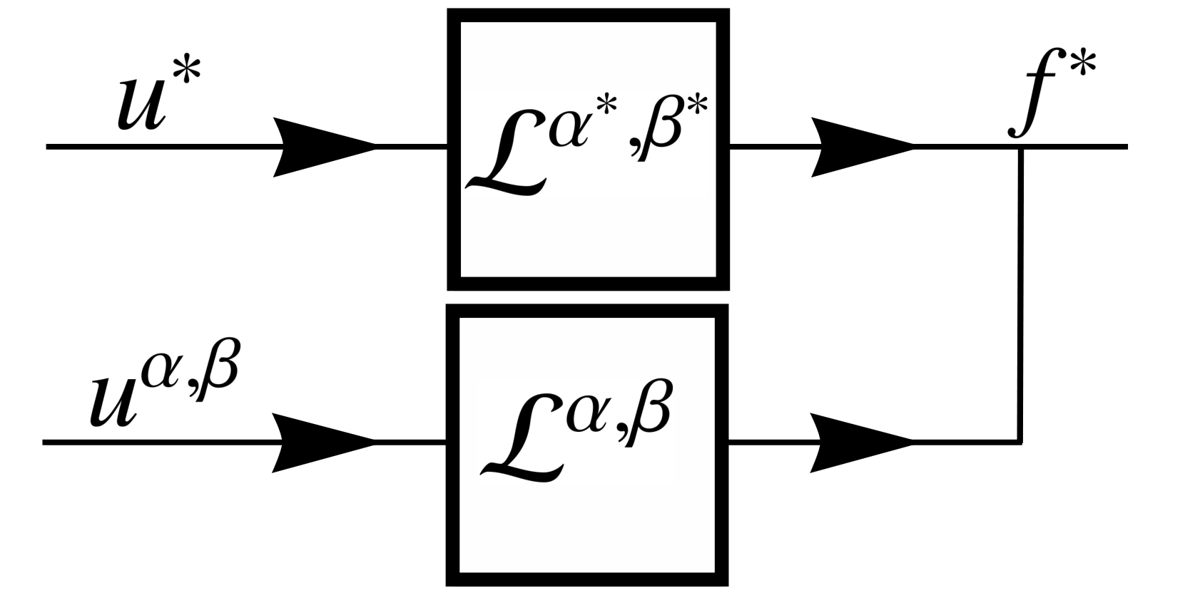
The fractional model can be simply visualized as Fig. 2, where ℒq​u=f\mathcal{L}^{q}u=f. We denote by the superscript (∗)(^{*}) as the exact values of quantities. Therefore, ℒq∗​u∗=f∗\mathcal{L}^{q^{*}}u^{*}=f^{*}, where u∗u^{*}, f∗f^{*} are the exact solution and force functions, respectively, and q∗q^{*} is the set of exact model parameters. Obviously, by choosing different values of model parameters (fractional indices), the fractional model observes the input differently, and thus, results in a different output. This leads to two types of model error, namely, type-I and type-II, described as follows. We note that the introduced model errors are zero at the exact values q∗q^{*}, by definition.

Refer to caption
Figure 2: Schematic of fractional model
Refer to caption
(a)
Refer to caption
(b)
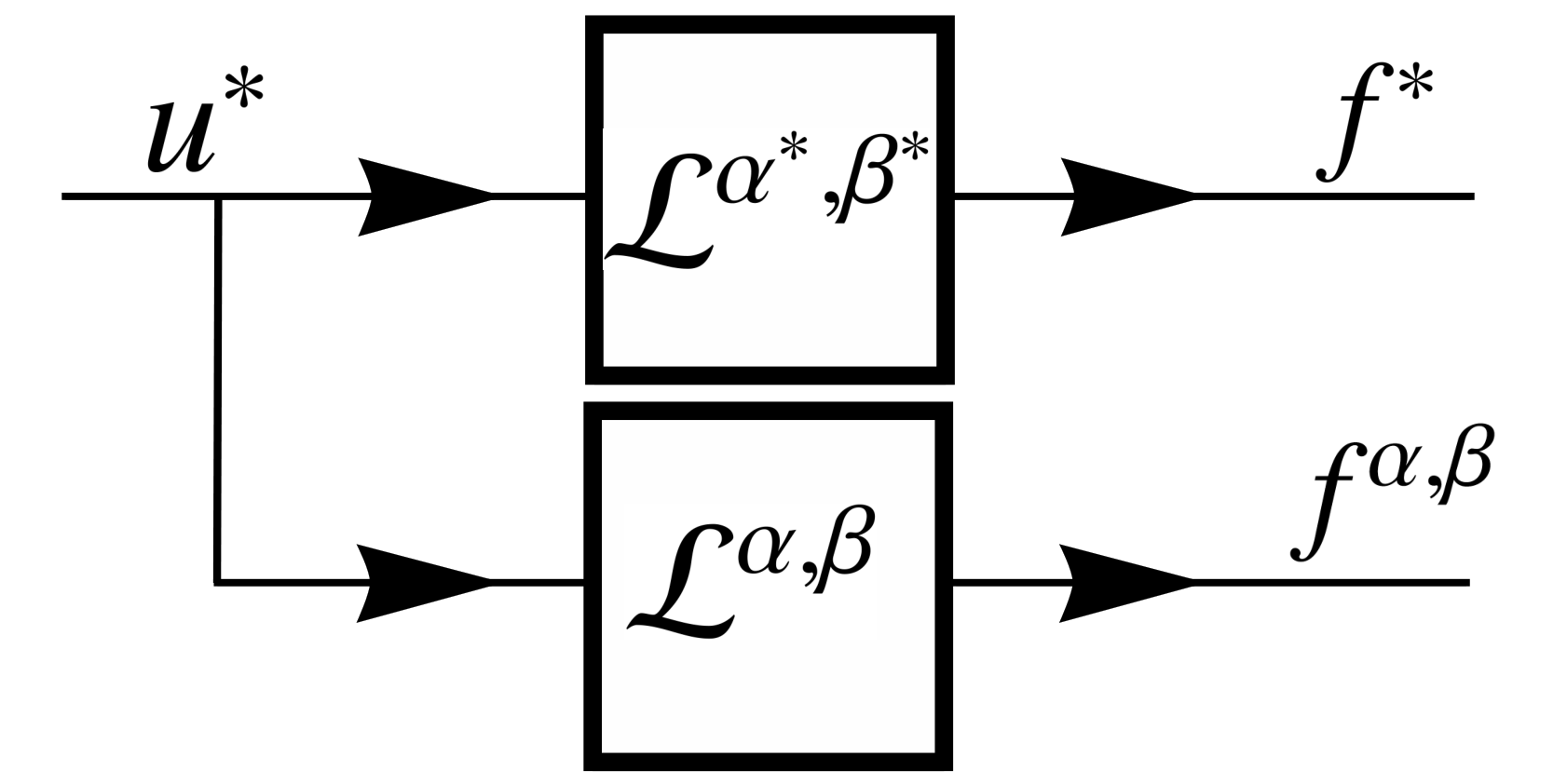
Figure 3: Schematic of variation of fractional model based on (a) model error type-I and (b) model error type-II.

5.1.1 Model Error: Type-I

In model error type-I, we consider the output of model to be fixed, i.e, f=f∗f=f^{*}, however, changing parameters makes the fractional model to observe the variated input uqu^{q} as opposed to u∗u^{*}. Therefore, we define the model error as the difference between variated and exact inputs, i.e. E⁡(q)=‖uq−u∗‖L2E(q)=||u^{q}-u^{*}||_{L^{2}}. The schematic of variation of model from the exact model is shown in Fig. 3 (a). For each variated model, we accurately compute the numerical approximation, uNqu_{N}^{q}, by solving (3.1), where by increasing the number of terms in the approximate solution, we make sure that the function E⁡(q)=‖uNq−u∗‖L2E(q)=||u_{N}^{q}-u^{*}||_{L^{2}} solely describes the model error with minimum discretization error. The proposed iterative algorithm, as will be discussed later, involves the gradient of model error with respect to the model parameters. Thus, we take the partial derivative of EE with respect to qq, as

SE,q=∂E∂q=∫ΩSuq,q​(uNq−u∗)​𝑑ΩE\displaystyle S_{E,q}=\frac{\partial E}{\partial q}=\frac{\int_{\Omega}S_{u^{q},q}\,(u_{N}^{q}-u^{*})\,\,d\Omega}{E} (5.1)

where Suq,q{S}_{u^{q},q} denotes the sensitivity fields, which is numerically obtained by solving FSEs (4.11). We note that in this case, since ff is fixed and therefore, not sensitive to any parameter, we exclude the first term in the definition of force functions fα\text{f}_{\alpha} and fβ\text{f}_{\beta}.

5.1.2 Model Error: type-II

In model error type-II, we consider the input of model to be fixed, i.e, u=u∗u=u^{*}, however, changing parameters makes the fractional model to result in the variated output fqf^{q} as opposed to f∗f^{*}. Therefore, we define the model error as the difference between variated and exact outputs, i.e. E⁡(q)=‖fq−f∗‖L2E(q)=||f^{q}-f^{*}||_{L^{2}}. The schematic of variation of model from the exact model is shown in Fig. 3 (b). In this case, unlike model error type-I, the model error and its gradient can be expressed analytically. Therefore, they do not contain any discretization error.

5.2 Model Error Minimization: Iterative Algorithm

We minimize the model error by formulating a two-stages algorithm. Since we do not have prior information about the variated solution/force function, it is difficult to analytically predict the behavior of introduced model error. However, in every example, we numerically study the behavior of a low resolution model error manifold on a coarse grid, and then, perform the local minimization. The minimization problem is written as:

minq∈Q​(E​(q)),\displaystyle\underset{q\,\in\,Q}{\min}\,\Big(\,E(q)\,\Big), (5.2)

in which E⁡(q):Q→ℝE(q):Q\rightarrow\mathbb{R}, and we assume that the problem is solvable, i.e. there exist a minimum point q∗∈Qq^{*}\in Q. Proper choice of initial guess in local minimization is of great importance, where a wrong initial guess, not falling within small enough adjacency of minimum, may never converge. Therefore, the iterative convergence in a hypercube space of parameters is highly connected to an optimal initial guess for each parameter. In the sequel, we delineate the two stages of our algorithm, namely, stage I: coarse grid searching, and stage II: nearby solution.

In stage I, we progressively divide the hypercube parameter space into subspaces to narrow down the objective search region into a smaller region. This division process is not necessarily unique and can be done in different ways, among which we discuss the easy-to-implement one here, where in each progression step, we choose the subspace with minimum error at its corner. We carry out the coarse grid searching till we reach a small enough region, in which the nearby solution (stage II) is valid. As an example, we consider a (1+1)(1+1)-D fractional model with q∗={α∗,β∗}={0.3,0.8}q^{*}=\{\alpha^{*},\beta^{*}\}=\{0.3,0.8\} as the exact fractional indices in the parameter surface, shown in Fig. 4. We divide the parameter space into four equal subspaces and by computing the error at corner points of each subsurface (black dots), we shrink the search region (to the labeled subsurface 33). We progress further once again in a similar fashion, divide the subsurface, and compute the error at corner points (red dots). We finally, narrow down the search region into labeled subsurface 3131. We see that in this case, with computing the error only at 14 points, we can efficiently narrow down the parameter space into a small enough search region, in which we can perform stage II of the algorithm.

α\alphaβ\beta
Figure 4: Iterative algorithm: coarse grid searching for (1+1)(1+1)-D parameter space, where α∗=0.3\alpha^{*}=0.3 and β∗=0.8\beta^{*}=0.8.

In stage II of the algorithm, we employ a gradient decent method, in which by starting from an initial guess q0={α0,β10,β20,⋯,βd0}q^{0}=\{\alpha^{0},\beta_{1}^{0},\beta_{2}^{0},\cdots,\beta_{d}^{0}\} in the obtained search region from stage I, we produce a minimizing sequence qi,i=1,2,⋯q^{i},\,i=1,2,\cdots, where

qi+1=qi+Δ​qi,\displaystyle q^{i+1}=q^{i}+\Delta q^{i}, (5.3)

and the increment Δ​qi=si​pi\Delta q^{i}=s^{i}p^{i} contains both the step size sis^{i} and normalized step direction pip^{i}. The superscript ii indicates the iteration index. We obtain the normalized direction pip^{i} by computing the gradient of model error with respect to the parameters. The step size is usually computed by performing a line search such that E⁡(qi+s​pi)E(q^{i}+s\,p^{i}) is minimized over ∀s∈ℝ\forall s\in\mathbb{R}. However, in our case the method does not produce well-scaled search directions, and we need to approximate the current step size, using the previous one. Thus,

pi=−∇E​(qi)‖∇E​(qi)‖,si=si−1​∇E(qi−1)Tpi−1∇E(qi)Tpi,\displaystyle p^{i}=-\frac{\nabla E(q^{i})}{\|\nabla E(q^{i})\|},\qquad s^{i}=s^{i-1}\frac{{\nabla E(q^{i-1})}^{T}\,p^{i-1}}{{\nabla E(q^{i})}^{T}\,p^{i}}, (5.4)

where the first iteration size is obtained, using the Taylor expansion of model error about q0q^{0}.

5.3 Fractional Model Construction: FSEM-based Iterative Algorithm

Let Ω=[0,T]×[−1,1]\Omega=[0,T]\times[-1,1] be the computational domain. We consider the (1+1)(1+1)-D case of FPDE (3.1), subject to the initial and boundary conditions (3.2) and (3.3), respectively, where the adjoint FSEs are given in (4.11). Assuming that the exact transport field u∗​(t,x)u^{*}(t,x) and force function f∗​(t,x)f^{*}(t,x) are given, then,

𝒟α∗t0​u∗−k⁡(𝒟β∗x−1+𝒟β∗1x)​u∗=f∗\displaystyle\prescript{}{0}{\mathcal{D}}_{t}^{\alpha^{*}}u^{*}-k\left(\,\prescript{}{-1}{\mathcal{D}}_{x}^{\beta^{*}}+\,\prescript{}{x}{\mathcal{D}}_{1}^{\beta^{*}}\right)u^{*}=f^{*} (5.5)

in which {α∗,β∗}\{\alpha^{*},\beta^{*}\} are the exact fractional indices and the coefficient kk is known.

By considering the two types of model error, we use the developed iterative formulation and follow Algorithm 1 and Algorithm 2 to obtain the optimal model parameters. In each iteration, the increments are obtained, using (5.4).

Algorithm 1 Fractional Model Construction: FSEM based Iterative Algorithm (Model Error type-I)
1:  Initial guess q0={α0,β0}q^{0}=\{\alpha^{0},\beta^{0}\}
2:  Do i=0,1,⋯i=0,1,\cdots
3:   Solve for uNqiu^{q^{i}}_{N}: FPDE
4:   Compute the model error E=‖uNqi−u∗‖L2E=||u_{N}^{q^{i}}-u^{*}||_{L^{2}}
5:    If E<toleranceE<\text{tolerance}, Then Break, Otherwise Continue
6:   Solve for sensitivity fields: FSEs
7:   Compute the model error gradient using sensitivity field
8:   Compute the iteration increment Δ​qi\Delta q^{i}
9:   March in parameter space qi+1=qi+Δ​qiq^{i+1}=q^{i}+\Delta q^{i}
10:  End
Algorithm 2 Fractional Model Construction: FSEM based Iterative Algorithm (Model Error type-II)
1:   Initial guess q0={α0,β0}q^{0}=\{\alpha^{0},\beta^{0}\}
2:  Do i=0,1,⋯i=0,1,\cdots
3:   Compute the model error E=‖ℒqi​u∗−ℒq∗​u∗‖L2E=||\mathcal{L}^{q^{i}}u^{*}-\mathcal{L}^{q^{*}}u^{*}||_{L^{2}}
4:    If E<toleranceE<\text{tolerance}, Then Break, Otherwise Continue
5:   Compute the model error gradient using sensitivity field (analytically available)
6:   Compute the iteration increment Δ​qi\Delta q^{i}
7:   March in parameter space qi+1=qi+Δ​qiq^{i+1}=q^{i}+\Delta q^{i}
8:  End
Remark 5.1.

In the first iteration, we compute the step size, using the Taylor expansion of the model error about the initial guess {α0,β0}{\{\alpha^{0},\beta^{0}\}}, which we separate into two directions as

E|{α∗,β∗}≈E|{α0,β0}+SE,α|{α0,β0}​(α∗−α0),E|{α∗,β∗}≈E|{α0,β0}+SE,β|{α0,β0}​(β∗−β0).\displaystyle E\Big|_{\{\alpha^{*},\beta^{*}\}}\approx E\Big|_{\{\alpha^{0},\beta^{0}\}}+S_{E,\alpha}\Big|_{\{\alpha^{0},\beta^{0}\}}\,\,(\alpha^{*}-\alpha^{0}),\qquad E\Big|_{\{\alpha^{*},\beta^{*}\}}\approx E\Big|_{\{\alpha^{0},\beta^{0}\}}+S_{E,\beta}\Big|_{\{\alpha^{0},\beta^{0}\}}\,\,(\beta^{*}-\beta^{0}). (5.6)

Knowing that E|{α∗,β∗}=0E\Big|_{\{\alpha^{*},\beta^{*}\}}=0, we obtain the parameters at next iterations as α1=α0+Δ​α0\alpha^{1}=\alpha^{0}+\Delta\alpha^{0} and β1=β0+Δ​β0\beta^{1}=\beta^{0}+\Delta\beta^{0}, in which

Δ​α0≈−E|{α0,β0}SE,α|{α0,β0},Δ​β0≈−E|{α0,β0}SE,β|{α0,β0}.\displaystyle\Delta\alpha^{0}\approx\,-\frac{E\Big|_{\{\alpha^{0},\beta^{0}\}}}{S_{E,\alpha}\Big|_{\{\alpha^{0},\beta^{0}\}}}\,\,,\qquad\qquad\Delta\beta^{0}\approx\,-\frac{E\Big|_{\{\alpha^{0},\beta^{0}\}}}{S_{E,\beta}\Big|_{\{\alpha^{0},\beta^{0}\}}}. (5.7)

6 Numerical Results

In the first part of numerical results, we investigate the performance of developed PG scheme in solving FPDE and the adjoint FSEs. We consider the coupled (1+1)(1+1)-d FPDE and FSEs with one-sided fractional derivative and k=1k=1, as

𝒟αt0​u−𝒟βx−1​u=f,\displaystyle\prescript{}{0}{\mathcal{D}}_{t}^{\alpha}u-\prescript{}{-1}{\mathcal{D}}_{x}^{\beta}\,u=f, (6.1)
𝒟αt0​Su,α−𝒟βx−1​Su,α=Sf,α−𝒜1​(α)​𝒟αt0​u+𝒟tα0L​P​u,\displaystyle\prescript{}{0}{\mathcal{D}}_{t}^{\alpha}S_{u,\alpha}-\prescript{}{-1}{\mathcal{D}}_{x}^{\beta}S_{u,\alpha}=S_{f,\alpha}-\mathcal{A}_{1}(\alpha)\prescript{}{0}{\mathcal{D}}_{t}^{\alpha}u+\prescript{LP}{0}{\mathcal{D}}_{t}^{\alpha}u, (6.2)
𝒟αt0​Su,β−𝒟βx−1​Su,β=Sf,β+𝒜2​(β)​𝒟βx−1​u−𝒟xβ−1L​P​u.\displaystyle\prescript{}{0}{\mathcal{D}}_{t}^{\alpha}S_{u,\beta}-\prescript{}{-1}{\mathcal{D}}_{x}^{\beta}S_{u,\beta}=S_{f,\beta}+\mathcal{A}_{2}(\beta)\,\prescript{}{-1}{\mathcal{D}}_{x}^{\beta}u-\prescript{LP}{-1}{\mathcal{D}}_{x}^{\beta}u. (6.3)

We consider two cases of exact solution as

  • •

    Case I: ue​x​t​(t,x)=t3+α/2​((1+x)3+β/2−12​(1+x)4+β/2)u^{ext}(t,x)=t^{3+\alpha/2}\,\left((1+x)^{3+\beta/2}-\frac{1}{2}(1+x)^{4+\beta/2}\right),

  • •

    Case II: ue​x​t​(t,x)=t3+α/2​(t−0.4)​(t−0.9)​((1+x)3+β/2−12​(1+x)4+β/2)u^{ext}(t,x)=t^{3+\alpha/2}(t-0.4)(t-0.9)\,\,\left((1+x)^{3+\beta/2}-\frac{1}{2}(1+x)^{4+\beta/2}\right).

where α/2=0.25\alpha/2=0.25, and β/2=0.75\beta/2=0.75. The exact solution and sensitivity fields, obtained by taking ∂∂α\frac{\partial}{\partial\alpha} and ∂∂β\frac{\partial}{\partial\beta} of the exact solutions, are shown in Fig. 5 and 6 for the two cases I and II, respectively. We employ the developed PG method to solve FPDE (6.1) and obtain uNu_{N}, which we use to construct the right hand side of adjoint FSEs. Then, we again employ the developed PG method to solve FSEs (6.2) and (6.3) and obtain the numerical sensitivity fields, SNu,α,SNu,βS_{N_{u,\alpha}},\,S_{N_{u,\beta}}. We study the L2L^{2}-norm convergence of our proposed method by increasing the number of basis functions, as shown in Fig. 7.

Refer to caption
Refer to caption
Refer to caption
Figure 5: Plot of exact functions for case I with α/2=0.25\alpha/2=0.25 and β/2=0.75\beta/2=0.75: exact solution ue​x​tu^{ext} (left), exact sensitivity field Sue​x​t,α=∂ue​x​t∂αS_{u^{ext},\alpha}=\frac{\partial u^{ext}}{\partial\alpha} (middle), exact sensitivity field Sue​x​t,β=∂ue​x​t∂βS_{u^{ext},\beta}=\frac{\partial u^{ext}}{\partial\beta} (right).
Refer to caption
Refer to caption
Refer to caption
Figure 6: Plot of exact functions for case II with α/2=0.25\alpha/2=0.25 and β/2=0.75\beta/2=0.75: exact solution ue​x​tu^{ext} (left), exact sensitivity field Sue​x​t,αS_{u^{ext},\alpha} (middle), exact sensitivity field Sue​x​t,βS_{u^{ext},\beta} (right).
Figure 7: PG spectral method, L2L^{2}-norm convergence study: (1+1)(1+1)-d FPDE adjoint to corresponding FSEs with one-sided fractional derivative, k=1k=1, α/2=0.25\alpha/2=0.25, and β/2=0.75\beta/2=0.75, for Case I (left) and Case II (right), where N=MN=M.

∙\bullet Fractional Model Construction. The second part of numerical results is dedicated to study the efficiency of developed iterative algorithm in obtaining the set of model parameters qq (fractional indices) and thus, construct the fractional model. We test our developed scheme by method of fabricated solution, assuming a given set of input (exact solution) and output (force term) for our fractional model.

We begin with a fractional IVP of the form 𝒟αt0​u​(t)=f⁡(t)\prescript{}{0}{\mathcal{D}}_{t}^{\alpha}u(t)=f(t), α∈(0,1)\alpha\in(0,1), and assume that the exact solution and force function are given as,

u∗​(t)=s​i​n​(5​π​α∗/2)​t3+α∗/2,\displaystyle u^{*}(t)=sin(5\pi\,\alpha^{*}/2)\,t^{3+\alpha^{*}/2},
f∗​(t)=s​i​n​(5​π​α∗/2)​Γ⁡(4+α∗/2)Γ⁡(4−α∗/2)​t3−α∗/2,\displaystyle f^{*}(t)=sin(5\pi\,\alpha^{*}/2)\,\frac{\Gamma(4+\alpha^{*}/2)}{\Gamma(4-\alpha^{*}/2)}\,t^{3-\alpha^{*}/2},

and the fractional order α\alpha is the unknown model parameter. We start from an initial guess α0\alpha^{0} and use the developed iterative algorithm to converge to the true value of fractional index α\alpha. We also consider a fractional BVP of the form 𝒟βx−1​u​(x)=f⁡(x)\prescript{}{-1}{\mathcal{D}}_{x}^{\beta}u(x)=f(x), β∈(1,2)\beta\in(1,2), and assume that the exact solution and force function are given as,

u∗​(x)=(1+x)3+β∗/2−12​(1+x)4+β∗/2\displaystyle u^{*}(x)=(1+x)^{3+\beta^{*}/2}-\frac{1}{2}(1+x)^{4+\beta^{*}/2}
f∗​(x)=Γ⁡(4+β∗/2)Γ⁡(4−β∗/2)​(1+x)3+β∗/2−12​Γ⁡(5+β∗/2)Γ⁡(5−β∗/2)​(1+x)4+β∗/2\displaystyle f^{*}(x)=\frac{\Gamma(4+\beta^{*}/2)}{\Gamma(4-\beta^{*}/2)}(1+x)^{3+\beta^{*}/2}-\frac{1}{2}\frac{\Gamma(5+\beta^{*}/2)}{\Gamma(5-\beta^{*}/2)}(1+x)^{4+\beta^{*}/2}

and the fractional order β\beta is the unknown model parameter. We again use the developed iterative algorithm to capture the true value of fractional index β\beta, starting from an initial guess β0\beta^{0}.

Tables 1 and 2 show two examples for each case of fractional IVP and BVP, where the true values of fractional orders are α∗=0.3\alpha^{*}=0.3, α∗=0.9\alpha^{*}=0.9, β∗=1.1\beta^{*}=1.1, and β∗=1.7\beta^{*}=1.7. We observe that the proposed iterative formulation converges accurately to the exact values with in few numbers of iterations. We note that in the case of fractional IVP and BVP, the search region is already small enough so that the nearby solution is valid, and therefore, we only need to perform the second stage of iterative algorithm.

Table 1: Fractional model construction for the two cases of fractional IVP.
Iteration Index     𝒟αt0​u​(t)=f⁡(t)\prescript{}{0}{\mathcal{D}}_{t}^{\alpha}u(t)=f(t)
i     αi\alpha^{i}     αi\alpha^{i}
initial guess     0.3000000.300000     0.9000000.900000
1     0.9719800.971980     0.3205200.320520
2     0.9004180.900418     0.3000680.300068
3     0.9000000.900000     0.3000000.300000
True Value     0.90.9     0.30.3
Table 2: Fractional model construction for the two cases of fractional BVP.
Iteration Index     𝒟βx−1​u​(x)=f⁡(x)\prescript{}{-1}{\mathcal{D}}_{x}^{\beta}u(x)=f(x)
i     βi\beta^{i}     βi\beta^{i}
initial guess     1.1000001.100000     1.90000001.9000000
1     1.8820201.882020     1.2280401.228040
2     1.7081201.708120     1.1060961.106096
3     1.7000201.700020     1.1000161.100016
4     1.7000001.700000     1.1000001.100000
True Value     1.71.7     1.11.1

Moreover, we consider FPDE of the form 𝒟αt0​u−k​𝒟βx−1​u=f\prescript{}{0}{\mathcal{D}}_{t}^{\alpha}u-k\prescript{}{-1}{\mathcal{D}}_{x}^{\beta}\,u=f. We assume the exact solution u∗=t1+α∗/2​((1+x)3+β∗/2−12​(1+x)4+β∗/2)u^{*}=t^{1+\alpha^{*}/2}\left((1+x)^{3+\beta^{*}/2}-\frac{1}{2}(1+x)^{4+\beta^{*}/2}\right) and plug it into the FPDE with given {α∗,β∗}\{\alpha^{*},\beta^{*}\} to obtain the exact force function f∗f^{*}. We study the example, in which, {α∗,β∗}={0.1,1.64}\{\alpha^{*},\beta^{*}\}=\{0.1,1.64\}. We perform the two stages of iterative algorithm, where in the first stage, we shrink down the search region 16 time smaller than the original size, by computing the model error at 8 points (See Fig. 8, right). Then, in the next stage, we start from the initial guess {α0,β0}={0.125,1.75}\{\alpha^{0},\beta^{0}\}=\{0.125,1.75\}, and observe that the developed iterative method converges to a close neighborhood of true values {0.1,1.64}\{0.1,1.64\} within 10−310^{-3} tolerance.

Refer to caption
Figure 8: Fractional model construction for the case FPDE, using FSEM based iterative algorithm. The true values of fractional indices are {α∗,β∗}={0.1,1.64}\{\alpha^{*},\beta^{*}\}=\{0.1,1.64\}.

The developed model construction method can also be applied in formulating fractional models to study complex time-varying nonlinear fluid-solid interaction phenomena [5, 3, 2] and also the effect of damping in structural vibrations [65, 1].

7 Summary

We developed a fractional sensitivity equation method (FSEM) in order to analyze the sensitivity of fractional models (FIVPs, FBVPs, and FPDEs) with respect to their parameters. We derived the adjoint governing dynamics of sensitivity coefficients, i.e. fractional sensitivity equations (FSEs), by taking the partial derivative of FDE with respect to the model parameters, and showed that they preserve the structure of original FDE. We also introduced a new fractional operator, associated with logarithmic-power law kernel, for the first time in the context of FSEM. We extended the existing proper underlying function spaces to respect the extra regularities imposed by FSEs and proved the well-posedness of problem. Moreover, we developed a Petrov-Galerkin (PG) spectral method by employing Jacobi polyfractonomials and Legendre polynomials as basis/test functions, and proved its stability. We further used the developed FSEM to formulate an optimization problem in order to construct the fractional model by estimating the model parameters. We defined two types of model error as objective functions and proposed a two-stages search algorithm to minimize them. We presented the steps of iterative algorithm in a pseudo code. Finally, we examined the performance of proposed numerical scheme in solving coupled FPDE and FSEs, where we numerically study the convergence rate of error. We also investigated the efficiency of developed iterative algorithm in estimating the derivative order for different cases of fractional models.

Appendix A Proof of Lemma (2.2)

Part A: σ∈(0,1)\sigma\in(0,1). We start from the R​L−P​LRL-PL definition, given in (2.8).

𝒟xσaR​L−L​P​u\displaystyle\prescript{RL-LP}{a}{\mathcal{D}}_{x}^{\sigma}u =1Γ⁡(1−σ)​dd​x​∫ax(x−s)−σ​log⁡(x−s)​u​(s)​𝑑s, (integrate by parts)\displaystyle=\frac{1}{\Gamma(1-\sigma)}\frac{d}{dx}\int_{a}^{x}\,(x-s)^{-\sigma}\,\log(x-s)\,u(s)\,ds,\,\text{ (integrate by parts)} (A.1)
=1Γ⁡(1−σ)dd​x{u⁡(s)​(x−s)1−σ(−σ+1)2(1−(−σ+1)log(x−s))|s=as=x\displaystyle=\frac{1}{\Gamma(1-\sigma)}\frac{d}{dx}\Big\{\frac{u(s)\,(x-s)^{1-\sigma}}{(-\sigma+1)^{2}}(1-(-\sigma+1)\,\log(x-s))\Bigg|_{s=a}^{s=x}
−∫ax(x−s)−σ+1(−σ+1)2(1−(−σ+1)log(x−s))u′(s)ds},\displaystyle\qquad-\int_{a}^{x}\,\frac{(x-s)^{-\sigma+1}}{(-\sigma+1)^{2}}\,(1-(-\sigma+1)\,\log(x-s))\,u^{\prime}(s)\,ds\Big\},
=1Γ⁡(1−σ)dd​x{u⁡(a)​(x−a)1−σ(−σ+1)2(1−(−σ+1)log(x−a))\displaystyle=\frac{1}{\Gamma(1-\sigma)}\frac{d}{dx}\Big\{\frac{u(a)\,(x-a)^{1-\sigma}}{(-\sigma+1)^{2}}(1-(-\sigma+1)\,\log(x-a))
−∫ax(x−s)−σ+1(−σ+1)2(1−(−σ+1)log(x−s))u′(s)ds},\displaystyle\qquad-\int_{a}^{x}\,\frac{(x-s)^{-\sigma+1}}{(-\sigma+1)^{2}}\,(1-(-\sigma+1)\,\log(x-s))\,u^{\prime}(s)\,ds\Big\},
=u⁡(a)Γ⁡(1−σ)​log⁡(x−a)(x−a)σ+1Γ⁡(1−σ)​∫axlog⁡(x−s)(x−s)−σ​u′​(s)​𝑑s, (by Leibnitz rule)\displaystyle=\frac{u(a)}{\Gamma(1-\sigma)}\,\frac{\log(x-a)}{(x-a)^{\sigma}}+\frac{1}{\Gamma(1-\sigma)}\int_{a}^{x}\,\frac{\log(x-s)}{(x-s)^{-\sigma}}\,u^{\prime}(s)\,ds,\,\text{ (by Leibnitz rule)}
=u⁡(a)Γ⁡(1−σ)​log⁡(x−a)(x−a)σ+𝒟xσaC−L​P​u\displaystyle=\frac{u(a)}{\Gamma(1-\sigma)}\,\frac{\log(x-a)}{(x-a)^{\sigma}}+\prescript{C-LP}{a}{\mathcal{D}}_{x}^{\sigma}u

Part B: σ∈(1,2)\sigma\in(1,2). Similarly, we start from the R​L−P​LRL-PL definition, given in (2.8).

𝒟xσaR​L−L​P​u\displaystyle\prescript{RL-LP}{a}{\mathcal{D}}_{x}^{\sigma}u =1Γ⁡(2−σ)​d2d​x2​∫ax(x−s)−σ+1​log⁡(x−s)​u​(s)​𝑑s, (integrate by parts twice)\displaystyle=\frac{1}{\Gamma(2-\sigma)}\frac{d^{2}}{dx^{2}}\int_{a}^{x}\,(x-s)^{-\sigma+1}\,\log(x-s)\,u(s)\,ds,\,\text{ (integrate by parts twice)} (A.2)
=1Γ⁡(2−σ)d2d​x2{u⁡(s)​(x−s)−σ+2(−σ+2)2(1−(−σ+2)log(x−s))|s=as=x\displaystyle=\frac{1}{\Gamma(2-\sigma)}\frac{d^{2}}{dx^{2}}\Big\{\frac{u(s)\,(x-s)^{-\sigma+2}}{(-\sigma+2)^{2}}(1-(-\sigma+2)\log(x-s))\Bigg|_{s=a}^{s=x}
−u′​(s)​(x−s)−σ+3(−σ+2)2​(−σ+3)2​(1−2​(−σ+3)+(−σ+3)​(−σ+2)​log⁡(x−s))|s=as=x\displaystyle\qquad-\frac{u^{\prime}(s)\,(x-s)^{-\sigma+3}}{(-\sigma+2)^{2}(-\sigma+3)^{2}}\left(1-2(-\sigma+3)+(-\sigma+3)(-\sigma+2)\log(x-s)\right)\Bigg|_{s=a}^{s=x}
+∫ax(x−s)−σ+3(−σ+2)2​(−σ+3)2(1−2(−σ+3)+(−σ+3)(−σ+2)log(x−s))u′′(s)ds},\displaystyle\qquad+\int_{a}^{x}\,\frac{(x-s)^{-\sigma+3}}{(-\sigma+2)^{2}(-\sigma+3)^{2}}\,\left(1-2(-\sigma+3)+(-\sigma+3)(-\sigma+2)\log(x-s)\right)\,u^{\prime\prime}(s)\,ds\Big\},
=1Γ⁡(2−σ)d2d​x2{u⁡(a)​(x−a)−σ+2(−σ+2)2(1−(−σ+2)log(x−a))\displaystyle=\frac{1}{\Gamma(2-\sigma)}\frac{d^{2}}{dx^{2}}\Big\{\frac{u(a)\,(x-a)^{-\sigma+2}}{(-\sigma+2)^{2}}(1-(-\sigma+2)\log(x-a))
−u′​(a)​(x−a)−σ+3(−σ+2)2​(−σ+3)2​(1−2​(−σ+3)+(−σ+3)​(−σ+2)​log⁡(x−a))\displaystyle\qquad-\frac{u^{\prime}(a)\,(x-a)^{-\sigma+3}}{(-\sigma+2)^{2}(-\sigma+3)^{2}}\left(1-2(-\sigma+3)+(-\sigma+3)(-\sigma+2)\log(x-a)\right)
+∫ax(x−s)−σ+3(−σ+2)2​(−σ+3)2(1−2(−σ+3)+(−σ+3)(−σ+2)log(x−s))u′′(s)ds},\displaystyle\qquad+\int_{a}^{x}\,\frac{(x-s)^{-\sigma+3}}{(-\sigma+2)^{2}(-\sigma+3)^{2}}\,\left(1-2(-\sigma+3)+(-\sigma+3)(-\sigma+2)\log(x-s)\right)\,u^{\prime\prime}(s)\,ds\Big\},
=u⁡(a)Γ⁡(2−σ)​1+(−σ+1)​log⁡(x−a)(x−a)σ+u′​(a)Γ⁡(2−σ)​log⁡(x−a)(x−a)σ−1\displaystyle=\frac{u(a)}{\Gamma(2-\sigma)}\frac{1+(-\sigma+1)\log(x-a)}{(x-a)^{\sigma}}+\frac{u^{\prime}(a)}{\Gamma(2-\sigma)}\frac{\log(x-a)}{(x-a)^{\sigma-1}}
+1Γ⁡(2−σ)∫ax(x−s)−σ+1log(x−s)u′′(s)ds, (by Leibnitz rule)\displaystyle\qquad+\frac{1}{\Gamma(2-\sigma)}\int_{a}^{x}\,(x-s)^{-\sigma+1}\,\log(x-s)\,u^{\prime\prime}(s)\,ds,\,\text{ (by Leibnitz rule)}
=u⁡(a)Γ⁡(1−σ)​1+(−σ+1)​log⁡(x−a)(x−a)σ+u′​(a)Γ⁡(1−σ)​log⁡(x−a)(x−a)σ−1+𝒟xσaC−P​L​u.\displaystyle=\frac{u(a)}{\Gamma(1-\sigma)}\frac{1+(-\sigma+1)\log(x-a)}{(x-a)^{\sigma}}+\frac{u^{\prime}(a)}{\Gamma(1-\sigma)}\frac{\log(x-a)}{(x-a)^{\sigma-1}}+\prescript{C-PL}{a}{\mathcal{D}}_{x}^{\sigma}u.

Appendix B Proof of Lemma (2.3)

In Lemma 2.1 in [33] and also in [19], it is shown that ∥⋅∥Hσl​(Λ)\|\cdot\|_{{{}^{l}}H^{\sigma}(\Lambda)} and ∥⋅∥Hσr​(Λ)\|\cdot\|_{{{}^{r}}H^{\sigma}(\Lambda)} are equivalent. Therefore, for u∈Hσ​(Λ)u\in H^{\sigma}(\Lambda), there exist positive constants C1C_{1} and C2C_{2} such that

‖u‖Hσ​(Λ)≤C1​‖u‖Hσl​(Λ),‖u‖Hσ​(Λ)≤C2​‖u‖Hσr​(Λ),\displaystyle\|u\|_{{}H^{\sigma}(\Lambda)}\leq C_{1}\|u\|_{{{}^{l}}H^{\sigma}(\Lambda)},\quad\|u\|_{{}H^{\sigma}(\Lambda)}\leq C_{2}\|u\|_{{{}^{r}}H^{\sigma}(\Lambda)}, (B.1)

which leads to

‖u‖Hσ​(Λ)2\displaystyle\|u\|_{{}H^{\sigma}(\Lambda)}^{2} ≤C12​‖u‖Hσl​(Λ)2+C22​‖u‖Hσr​(Λ)2,\displaystyle\leq C_{1}^{2}\|u\|_{{{}^{l}}H^{\sigma}(\Lambda)}^{2}+C_{2}^{2}\|u\|_{{{}^{r}}H^{\sigma}(\Lambda)}^{2},
=C12​‖𝒟σxa​(u)‖L2​(Λ)2+C22​‖𝒟σbx​(u)‖L2​(Λ)2+(C12+C22)​‖u‖L2​(Λ)2,\displaystyle=C_{1}^{2}\,\|\prescript{}{a}{\mathcal{D}}_{x}^{\sigma}\,(u)\|_{L^{2}(\Lambda)}^{2}+C_{2}^{2}\,\|\prescript{}{x}{\mathcal{D}}_{b}^{\sigma}\,(u)\|_{L^{2}(\Lambda)}^{2}+(C_{1}^{2}+C_{2}^{2})\,\|u\|_{L^{2}(\Lambda)}^{2},
≤C~1​‖u‖Hσc​(Λ)2,\displaystyle\leq\tilde{C}_{1}\,\|u\|_{{{}^{c}}H^{\sigma}(\Lambda)}^{2}, (B.2)

where C~1\tilde{C}_{1} is a positive constant. Similarly, we can show that ‖u‖Hσc​(Λ)2≤C~2​‖u‖Hσ​(Λ)\|u\|_{{{}^{c}}H^{\sigma}(\Lambda)}^{2}\leq\tilde{C}_{2}\,\|u\|_{{}H^{\sigma}(\Lambda)}, where C~2\tilde{C}_{2} is a positive constant.

Appendix C Proof of Lemma (2.5)

𝒳1\mathcal{X}_{1} is endowed with the norm ∥⋅∥𝒳1\|\cdot\|_{\mathcal{X}_{1}}, where ∥⋅∥𝒳1≡∥⋅∥Hβ1/2c​(Λ1)\|\cdot\|_{\mathcal{X}_{1}}\equiv\|\cdot\|_{{{}^{c}}H^{\beta_{1}/2}(\Lambda_{1})} by Lemma 2.3. Moreover, 𝒳2\mathcal{X}_{2} is associated with the norm

∥⋅∥𝒳2≡{∥⋅∥H0β2/2c​((a2,b2),L2​(Λ1))2+∥⋅∥L2​((a2,b2),𝒳1)2}12,\|\cdot\|_{\mathcal{X}_{2}}\equiv\bigg\{\|\cdot\|_{{{}^{c}}H^{\beta_{2}/2}_{0}\Big((a_{2},b_{2});L^{2}(\Lambda_{1})\Big)}^{2}+\|\cdot\|_{L^{2}\Big((a_{2},b_{2});\mathcal{X}_{1}\Big)}^{2}\bigg\}^{\frac{1}{2}}, (C.1)

where

‖u‖H0β2/2c​((a2,b2),L2​(Λ1))2\displaystyle\|u\|_{{{}^{c}}H^{\beta_{2}/2}_{0}\Big((a_{2},b_{2});L^{2}(\Lambda_{1})\Big)}^{2} =∫a1b1(∫a2b2|𝒟β2/2x2a2​u|2​d​x2+∫a2b2|𝒟β2/2b2x2​u|2​d​x2+∫a2b2|u|2​d​x2)​d​x1\displaystyle=\int_{a_{1}}^{b_{1}}\,\Big(\int_{a_{2}}^{b_{2}}\,|\prescript{}{a_{2}}{\mathcal{D}}_{x_{2}}^{\beta_{2}/2}u|^{2}\,dx_{2}+\int_{a_{2}}^{b_{2}}\,|\prescript{}{x_{2}}{\mathcal{D}}_{b_{2}}^{\beta_{2}/2}u|^{2}\,dx_{2}+\int_{a_{2}}^{b_{2}}\,|u|^{2}\,dx_{2}\Big)\,dx_{1}
=∫a1b1∫a2b2|𝒟β2/2x2a2​u|2​d​x2​d​x1+∫a1b1∫a2b2|𝒟β2/2b2x2​u|2​d​x2​d​x1+∫a1b1∫a2b2|u|2​d​x2​d​x1\displaystyle=\int_{a_{1}}^{b_{1}}\int_{a_{2}}^{b_{2}}\,|\prescript{}{a_{2}}{\mathcal{D}}_{x_{2}}^{\beta_{2}/2}u|^{2}\,dx_{2}dx_{1}+\int_{a_{1}}^{b_{1}}\int_{a_{2}}^{b_{2}}\,|\prescript{}{x_{2}}{\mathcal{D}}_{b_{2}}^{\beta_{2}/2}u|^{2}\,dx_{2}dx_{1}+\int_{a_{1}}^{b_{1}}\int_{a_{2}}^{b_{2}}\,|u|^{2}\,dx_{2}dx_{1}
=‖𝒟β2/2b2x2​(u)‖L2​(Λd)2+‖𝒟β2/2x2a2​(u)‖L2​(Λd)2+‖u‖L2​(Λd)2,\displaystyle=\|\prescript{}{x_{2}}{\mathcal{D}}_{b_{2}}^{\beta_{2}/2}\,(u)\|_{L^{2}(\Lambda_{d})}^{2}+\|\prescript{}{a_{2}}{\mathcal{D}}_{x_{2}}^{\beta_{2}/2}\,(u)\|_{L^{2}(\Lambda_{d})}^{2}+\|u\|_{L^{2}(\Lambda_{d})}^{2}, (C.2)

and

‖u‖L2​((a2,b2),𝒳1)2\displaystyle\|u\|_{L^{2}\Big((a_{2},b_{2});\mathcal{X}_{1}\Big)}^{2}
=∫a2b2(∫a1b1|𝒟β1/2x1a1​u|2​d​x1+∫a1b1|𝒟β1/2b1x1​u|2​d​x1+∫a1b1|u|2​d​x1)​d​x2\displaystyle=\int_{a_{2}}^{b_{2}}\,\Big(\int_{a_{1}}^{b_{1}}\,|\prescript{}{a_{1}}{\mathcal{D}}_{x_{1}}^{\beta_{1}/2}u|^{2}\,dx_{1}+\int_{a_{1}}^{b_{1}}\,|\prescript{}{x_{1}}{\mathcal{D}}_{b_{1}}^{\beta_{1}/2}u|^{2}\,dx_{1}+\int_{a_{1}}^{b_{1}}\,|u|^{2}\,dx_{1}\Big)\,dx_{2}
=∫a2b2∫a1b1|𝒟β1/2x1a1​u|2​d​x1​d​x2+∫a2b2∫a1b1|𝒟β1/2b1x1​u|2​d​x1​d​x2+∫a2b2∫a1b1|u|2​d​x1​d​x2\displaystyle=\int_{a_{2}}^{b_{2}}\int_{a_{1}}^{b_{1}}|\prescript{}{a_{1}}{\mathcal{D}}_{x_{1}}^{\beta_{1}/2}u|^{2}dx_{1}dx_{2}+\int_{a_{2}}^{b_{2}}\int_{a_{1}}^{b_{1}}|\prescript{}{x_{1}}{\mathcal{D}}_{b_{1}}^{\beta_{1}/2}u|^{2}dx_{1}dx_{2}+\int_{a_{2}}^{b_{2}}\int_{a_{1}}^{b_{1}}|u|^{2}dx_{1}dx_{2}
=‖𝒟β1/2b1x1​u‖L2​(Λ2)2+‖𝒟β1/2x1a1​u‖L2​(Λ2)2+‖u‖L2​(Λ2)2.\displaystyle=\|\prescript{}{x_{1}}{\mathcal{D}}_{b_{1}}^{\beta_{1}/2}\,u\|_{L^{2}(\Lambda_{2})}^{2}+\|\prescript{}{a_{1}}{\mathcal{D}}_{x_{1}}^{\beta_{1}/2}\,u\|_{L^{2}(\Lambda_{2})}^{2}+\|u\|_{L^{2}(\Lambda_{2})}^{2}. (C.3)

We use the mathematical induction to carry out the proof. Therefore, we assume the following equality holds

∥⋅∥𝒳k−1≡{∑i=1k−1(∥𝒟biβi/2xi(⋅)∥L2​(Λk−1)2+∥𝒟xiβi/2ai(⋅)∥L2​(Λk−1)2)+∥⋅∥L2​(Λk−1)2}12.\|\cdot\|_{\mathcal{X}_{k-1}}\equiv\bigg\{\sum_{i=1}^{k-1}\Big(\|\prescript{}{x_{i}}{\mathcal{D}}_{b_{i}}^{\beta_{i}/2}\,(\cdot)\|_{L^{2}(\Lambda_{k-1})}^{2}+\|\prescript{}{a_{i}}{\mathcal{D}}_{x_{i}}^{\beta_{i}/2}\,(\cdot)\|_{L^{2}(\Lambda_{k-1})}^{2}\Big)+\|\cdot\|_{L^{2}(\Lambda_{k-1})}^{2}\bigg\}^{\frac{1}{2}}. (C.4)

Since,

‖u‖H0βk/2c​((ak,bk),L2​(Λk−1))2\displaystyle\|u\|_{{{}^{c}}H^{\beta_{k}/2}_{0}\Big((a_{k},b_{k});L^{2}(\Lambda_{k-1})\Big)}^{2}
=∫Λk−1(∫akbk|𝒟βk/2xkak​u|2​d​xk+∫akbk|𝒟βk/2bkxk​u|2​d​xk+∫akbk|u|2​d​xk)​d​Λk−1\displaystyle=\int_{\Lambda_{k-1}}\,\Big(\int_{a_{k}}^{b_{k}}\,|\prescript{}{a_{k}}{\mathcal{D}}_{x_{k}}^{\beta_{k}/2}u|^{2}\,dx_{k}+\int_{a_{k}}^{b_{k}}\,|\prescript{}{x_{k}}{\mathcal{D}}_{b_{k}}^{\beta_{k}/2}u|^{2}\,dx_{k}+\int_{a_{k}}^{b_{k}}\,|u|^{2}\,dx_{k}\Big)\,d\Lambda_{k-1}
=∫Λk−1∫akbk|𝒟βk/2xkak​u|2​d​xk​d​Λk−1+∫Λk−1∫akbk|𝒟βk/2bkxk​u|2​d​xk​d​Λk−1+∫Λk−1∫akbk|u|2​d​xk​d​Λk−1\displaystyle=\int_{\Lambda_{k-1}}\int_{a_{k}}^{b_{k}}\,|\prescript{}{a_{k}}{\mathcal{D}}_{x_{k}}^{\beta_{k}/2}u|^{2}\,dx_{k}d\Lambda_{k-1}+\int_{\Lambda_{k-1}}\int_{a_{k}}^{b_{k}}\,|\prescript{}{x_{k}}{\mathcal{D}}_{b_{k}}^{\beta_{k}/2}u|^{2}\,dx_{k}d\Lambda_{k-1}+\int_{\Lambda_{k-1}}\int_{a_{k}}^{b_{k}}\,|u|^{2}\,dx_{k}d\Lambda_{k-1}
=‖𝒟βk/2bkxk​(u)‖L2​(Λk)2+‖𝒟βk/2xkak​(u)‖L2​(Λk)2+‖u‖L2​(Λk)2,\displaystyle=\|\prescript{}{x_{k}}{\mathcal{D}}_{b_{k}}^{\beta_{k}/2}\,(u)\|_{L^{2}(\Lambda_{k})}^{2}+\|\prescript{}{a_{k}}{\mathcal{D}}_{x_{k}}^{\beta_{k}/2}\,(u)\|_{L^{2}(\Lambda_{k})}^{2}+\|u\|_{L^{2}(\Lambda_{k})}^{2},

and

‖u‖L2​((ak,bk),𝒳k−1)2\displaystyle\|u\|_{L^{2}\Big((a_{k},b_{k});\mathcal{X}_{k-1}\Big)}^{2} =∫akbk(∑i=1k−1(∫Λk−1|𝒟βi/2xiai​u|2​d​Λk−1+∫Λk−1|𝒟βi/2bixi​u|2​d​Λk−1)+∫Λk−1|u|2​d​Λk−1)​d​xk\displaystyle=\int_{a_{k}}^{b_{k}}\left(\sum_{i=1}^{k-1}\left(\int_{\Lambda_{k-1}}|\prescript{}{a_{i}}{\mathcal{D}}_{x_{i}}^{\beta_{i}/2}u|^{2}d\Lambda_{k-1}+\int_{\Lambda_{k-1}}|\prescript{}{x_{i}}{\mathcal{D}}_{b_{i}}^{\beta_{i}/2}u|^{2}d\Lambda_{k-1}\right)+\int_{\Lambda_{k-1}}|u|^{2}d\Lambda_{k-1}\right)dx_{k}
=∑i=1k−1(∫Λk|𝒟βi/2xiai​u|2​d​Λk+∫Λk|𝒟βi/2bixi​u|2​d​Λk)+∫Λk|u|2​d​Λk\displaystyle=\sum_{i=1}^{k-1}\Big(\int_{\Lambda_{k}}|\prescript{}{a_{i}}{\mathcal{D}}_{x_{i}}^{\beta_{i}/2}u|^{2}d\Lambda_{k}+\int_{\Lambda_{k}}|\prescript{}{x_{i}}{\mathcal{D}}_{b_{i}}^{\beta_{i}/2}u|^{2}d\Lambda_{k}\Big)+\int_{\Lambda_{k}}|u|^{2}d\Lambda_{k}
=∑i=1k−1(‖𝒟βi/2bixi​u‖L2​(Λk)2+‖𝒟βi/2xiai​u‖L2​(Λk)2)+‖u‖L2​(Λk)2,\displaystyle=\sum_{i=1}^{k-1}\Big(\|\prescript{}{x_{i}}{\mathcal{D}}_{b_{i}}^{\beta_{i}/2}\,u\|_{L^{2}(\Lambda_{k})}^{2}+\|\prescript{}{a_{i}}{\mathcal{D}}_{x_{i}}^{\beta_{i}/2}\,u\|_{L^{2}(\Lambda_{k})}^{2}\Big)+\|u\|_{L^{2}(\Lambda_{k})}^{2},

we can show that

∥⋅∥𝒳k≡{∑i=1k(∥𝒟biβi/2xi(⋅)∥L2​(Λk)2+∥𝒟xiβi/2ai(⋅)∥L2​(Λk)2)+∥⋅∥L2​(Λk)2}12.\|\cdot\|_{\mathcal{X}_{k}}\equiv\bigg\{\sum_{i=1}^{k}\Big(\|\prescript{}{x_{i}}{\mathcal{D}}_{b_{i}}^{\beta_{i}/2}\,(\cdot)\|_{L^{2}(\Lambda_{k})}^{2}+\|\prescript{}{a_{i}}{\mathcal{D}}_{x_{i}}^{\beta_{i}/2}\,(\cdot)\|_{L^{2}(\Lambda_{k})}^{2}\Big)+\|\cdot\|_{L^{2}(\Lambda_{k})}^{2}\bigg\}^{\frac{1}{2}}. (C.5)

Appendix D Proof of Lemma (2.8)

According to [30], we have 𝒟βixiai​u=𝒟βi/2xiai​(𝒟βi/2xiai​u)\prescript{}{a_{i}}{\mathcal{D}}_{x_{i}}^{\beta_{i}}u=\prescript{}{a_{i}}{\mathcal{D}}_{x_{i}}^{\beta_{i}/2}(\prescript{}{a_{i}}{\mathcal{D}}_{x_{i}}^{\beta_{i}/2}u) and 𝒟βi/2bixi​u=𝒟βi/2bixi​(𝒟βi/2bixi​u)\prescript{}{x_{i}}{\mathcal{D}}_{b_{i}}^{\beta_{i}/2}u=\prescript{}{x_{i}}{\mathcal{D}}_{b_{i}}^{\beta_{i}/2}(\prescript{}{x_{i}}{\mathcal{D}}_{b_{i}}^{\beta_{i}/2}u). Let u¯=𝒟βi/2xiai​u\bar{u}=\prescript{}{a_{i}}{\mathcal{D}}_{x_{i}}^{\beta_{i}/2}u. Then,

(𝒟βixiai​u,v)Λd\displaystyle(\prescript{}{a_{i}}{\mathcal{D}}_{x_{i}}^{\beta_{i}}u,v)_{\Lambda_{d}} =\displaystyle= (𝒟βi/2xiai​u¯,v)Λd=∫Λd1Γ⁡(1−βi/2)​[dd​xi​∫aixiu¯​(s)​d​s(xi−s)iβ/2]​v​d​Λd\displaystyle(\prescript{}{a_{i}}{\mathcal{D}}_{x_{i}}^{\beta_{i}/2}\bar{u},v)_{\Lambda_{d}}=\int_{\Lambda_{d}}\frac{1}{\Gamma(1-\beta_{i}/2)}\big[\frac{d}{dx_{i}}\,\int_{a_{i}}^{x_{i}}\frac{\bar{u}(s)\,ds}{(x_{i}-s)^{\beta}_{i}/2}\big]v\,d\Lambda_{d} (D.1)
=\displaystyle= {vΓ⁡(1−βi/2)​∫aixiu¯​d​s(xi−s)βi/2}xi=aibi−∫Λd1Γ⁡(1−βi/2)​∫aixiu¯​(s)​d​s(xi−s)βi/2​d​vd​xi​d​Λd.\displaystyle\Big\{\frac{v}{\Gamma(1-\beta_{i}/2)\int_{a_{i}}^{x_{i}}\frac{\bar{u}ds}{(x_{i}-s)^{\beta_{i}/2}}}\Big\}^{b_{i}}_{x_{i}=a_{i}}-\int_{\Lambda_{d}}\frac{1}{\Gamma(1-\beta_{i}/2)}\int_{a_{i}}^{x_{i}}\frac{\bar{u}(s)\,ds}{(x_{i}-s)^{\beta_{i}/2}}\frac{dv}{dx_{i}}\,d\Lambda_{d}.\quad\quad

Based on the homogeneous boundary conditions, {vΓ⁡(1−βi/2)​∫aixiu¯​d​s(xi−s)βi/2}xi=aibi=0.\Big\{\frac{v}{\Gamma(1-\beta_{i}/2)\int_{a_{i}}^{x_{i}}\frac{\bar{u}ds}{(x_{i}-s)^{\beta_{i}/2}}}\Big\}^{b_{i}}_{x_{i}=a_{i}}=0. Therefore,

(𝒟βixiai​u,v)Λd\displaystyle(\prescript{}{a_{i}}{\mathcal{D}}_{x_{i}}^{\beta_{i}}u,v)_{\Lambda_{d}} =\displaystyle= −∫Λi1Γ⁡(1−βi/2)∫aixiu¯​(s)​d​s(xi−s)βi/2d​vd​xidΛi.\displaystyle-\int_{\Lambda_{i}}\frac{1}{\Gamma(1-\beta_{i}/2)}\int_{a_{i}}^{x_{i}}\frac{\bar{u}(s)\,ds}{(x_{i}-s)^{\beta_{i}/2}}\frac{dv}{dx_{i}}\,d\Lambda_{i}. (D.2)

Moreover, we find that

dd​s​∫aibiu(xi−s)βi/2​d​xi\displaystyle\frac{d}{ds}\,\int_{a_{i}}^{b_{i}}\frac{u}{(x_{i}-s)^{\beta_{i}/2}}dx_{i} =\displaystyle= dd​s​{{v​(xi−s)1−βi/21−βi/2}xi=sibi−11−βi/2​∫sbid​vd​xi​(xi−s)1−βi/2​d​xi}\displaystyle\frac{d}{ds}\Big\{\{\frac{v\,(x_{i}-s)^{1-\beta_{i}/2}}{1-\beta_{i}/2}\}_{x_{i}=s_{i}}^{b_{i}}-\frac{1}{1-\beta_{i}/2}\int_{s}^{b_{i}}\frac{dv}{dx_{i}}(x_{i}-s)^{1-\beta_{i}/2}dx_{i}\Big\} (D.3)
=\displaystyle= −11−βi/2∫sbid​vd​xi(xi−s)1−βi/2dxi=∫sbid​vd​xi(xi−s)βi/2dxi.\displaystyle-\frac{1}{1-\beta_{i}/2}\int_{s}^{b_{i}}\frac{dv}{dx_{i}}(x_{i}-s)^{1-\beta_{i}/2}\,dx_{i}=\int_{s}^{b_{i}}\frac{\frac{dv}{dx_{i}}}{(x_{i}-s)^{\beta_{i}/2}}\,dx_{i}.

Therefore, we get

(𝒟xiβi/2aiu¯,v)Λd=−∫Λd1Γ​(1−ν)iu¯(s)(−dd​s∫sbiv(xi−s)βi/2dxi)ds=(u¯,𝒟biβi/2xiv)Λd.\displaystyle(\prescript{}{a_{i}}{\mathcal{D}}_{x_{i}}^{\beta_{i}/2}\bar{u},v)_{\Lambda_{d}}=-\int_{\Lambda_{d}}\frac{1}{\Gamma(1-\nu)_{i}}\,\bar{u}(s)\big(-\frac{d}{ds}\int_{s}^{b_{i}}\frac{v}{(x_{i}-s)^{\beta_{i}/2}}dx_{i}\big)\,ds=(\bar{u},\prescript{}{x_{i}}{\mathcal{D}}_{b_{i}}^{\beta_{i}/2}v)_{\Lambda_{d}}.\quad

Appendix E Proof of Lemma (4.4)

We know that

|(𝒟α/2t0​u,𝒟α/2Tt​v)Ω|=(∫Λd∫0T|𝒟α/2t0​u​𝒟α/2Tt​v|2​𝑑t​d​Λd)12.\displaystyle\big|\left(\prescript{}{0}{\mathcal{D}}_{t}^{\alpha/2}u,\prescript{}{t}{\mathcal{D}}_{T}^{\alpha/2}v\right)_{\Omega}\big|=\Big(\int_{\Lambda_{d}}\int_{0}^{T}|\prescript{}{0}{\mathcal{D}}_{t}^{\alpha/2}u\,\prescript{}{t}{\mathcal{D}}_{T}^{\alpha/2}v|^{2}\,dtd\Lambda_{d}\Big)^{\frac{1}{2}}.

Therefore, by Hölder inequality

|(𝒟α/2t0​u,𝒟α/2Tt​v)Ω|\displaystyle\big|\left(\prescript{}{0}{\mathcal{D}}_{t}^{\alpha/2}u,\prescript{}{t}{\mathcal{D}}_{T}^{\alpha/2}v\right)_{\Omega}\big|
≤(∫Λd∫0T|𝒟α/2t0​u|2​𝑑t​d​Λd)12​(∫Λd∫0T|𝒟α/2Tt​v|2​𝑑t​d​Λd)12\displaystyle\leq\Big(\int_{\Lambda_{d}}\int_{0}^{T}|\prescript{}{0}{\mathcal{D}}_{t}^{\alpha/2}u|^{2}\,dtd\Lambda_{d}\Big)^{\frac{1}{2}}\,\Big(\int_{\Lambda_{d}}\int_{0}^{T}|\prescript{}{t}{\mathcal{D}}_{T}^{\alpha/2}v|^{2}\,dtd\Lambda_{d}\Big)^{\frac{1}{2}}
≤(∫Λd∫0T|𝒟α/2t0​u|2​𝑑t​d​Λd+∫Λd∫0T|u|2​𝑑t​d​Λd)12​(∫Λd∫0T|𝒟α/2Tt​v|2​𝑑t​d​Λd+∫Λd∫0T|v|2​𝑑t​d​Λd)12\displaystyle\leq\Big(\int_{\Lambda_{d}}\int_{0}^{T}|\prescript{}{0}{\mathcal{D}}_{t}^{\alpha/2}u|^{2}\,dtd\Lambda_{d}+\int_{\Lambda_{d}}\int_{0}^{T}|u|^{2}\,dtd\Lambda_{d}\Big)^{\frac{1}{2}}\,\Big(\int_{\Lambda_{d}}\int_{0}^{T}|\prescript{}{t}{\mathcal{D}}_{T}^{\alpha/2}v|^{2}\,dtd\Lambda_{d}+\int_{\Lambda_{d}}\int_{0}^{T}|v|^{2}\,dtd\Lambda_{d}\Big)^{\frac{1}{2}}
=‖𝒟α/2t0​u‖L2​(Ω)​‖𝒟α/2Tt​v‖L2​(Ω)=‖u‖Hα/2l​(I,L2​(Λd))​‖v‖Hα/2r​(I,L2​(Λd)).\displaystyle=\|\prescript{}{0}{\mathcal{D}}_{t}^{\alpha/2}u\|_{L^{2}(\Omega)}\,\|\prescript{}{t}{\mathcal{D}}_{T}^{\alpha/2}v\|_{L^{2}(\Omega)}=\|u\|_{\prescript{l}{}{H}^{\alpha/2}(I;L^{2}(\Lambda_{d}))}\,\|v\|_{\prescript{r}{}{H}^{\alpha/2}(I;L^{2}(\Lambda_{d}))}.

Moreover, by equivalence of |⋅|Hs​(I)≡|⋅|∗Hs​(I)=|⋅|1/2Hsl​(I)|⋅|1/2Hsr​(I)|\cdot|_{H^{s}(I)}\equiv|\cdot|^{*}_{H^{s}(I)}=|\cdot|^{1/2}_{{{}^{l}}H^{s}(I)}|\cdot|^{1/2}_{{{}^{r}}H^{s}(I)} we have

|(𝒟α/2t0​u,𝒟α/2Tt​v)I|\displaystyle|(\prescript{}{0}{\mathcal{D}}_{t}^{\alpha/2}u,\prescript{}{t}{\mathcal{D}}_{T}^{\alpha/2}v)_{I}| =\displaystyle= ∫0T|𝒟α/2t0​u​𝒟α/2Tt​v|2​𝑑t\displaystyle\int_{0}^{T}|\prescript{}{0}{\mathcal{D}}_{t}^{\alpha/2}u\,\prescript{}{t}{\mathcal{D}}_{T}^{\alpha/2}v|^{2}\,dt (E.1)
≥\displaystyle\geq ∫0T|𝒟α/2t0​u|2​𝑑t​∫0T|𝒟α/2Tt​v|2​𝑑t≥β~1​‖u‖Hsl​(I)​‖v‖Hsr​(I),\displaystyle\int_{0}^{T}|\prescript{}{0}{\mathcal{D}}_{t}^{\alpha/2}u|^{2}dt\,\int_{0}^{T}|\prescript{}{t}{\mathcal{D}}_{T}^{\alpha/2}v|^{2}\,dt\geq\tilde{\beta}_{1}\|u\|_{{{}^{l}}H^{s}(I)}\|v\|_{{{}^{r}}H^{s}(I)},

where 0<β~1≤10<\tilde{\beta}_{1}\leq 1. Therefore,

|(𝒟α/2t0​u,𝒟α/2Tt​v)Ω|2\displaystyle|(\prescript{}{0}{\mathcal{D}}_{t}^{\alpha/2}u,\prescript{}{t}{\mathcal{D}}_{T}^{\alpha/2}v)_{\Omega}|^{2} =\displaystyle= ∫Λd∫0T|𝒟α/2t0​u​𝒟α/2Tt​v|2​𝑑t​d​Λd\displaystyle\int_{\Lambda_{d}}\int_{0}^{T}|\prescript{}{0}{\mathcal{D}}_{t}^{\alpha/2}u\,\prescript{}{t}{\mathcal{D}}_{T}^{\alpha/2}v|^{2}\,dt\,d\Lambda_{d} (E.2)
≥\displaystyle\geq ∫Λd(∫0T|𝒟α/2t0​u|2​𝑑t​∫0T|𝒟α/2Tt​v|2​𝑑t)​d​Λd\displaystyle\int_{\Lambda_{d}}\Big(\int_{0}^{T}|\prescript{}{0}{\mathcal{D}}_{t}^{\alpha/2}u|^{2}dt\,\int_{0}^{T}|\prescript{}{t}{\mathcal{D}}_{T}^{\alpha/2}v|^{2}\,dt\Big)\,d\Lambda_{d}
≥\displaystyle\geq β¯​∫Λd∫0T|𝒟α/2t0​u|2​𝑑t​d​Λd​∫Λd∫0T|𝒟α/2Tt​v|2​𝑑t​Λd\displaystyle\bar{\beta}\int_{\Lambda_{d}}\int_{0}^{T}|\prescript{}{0}{\mathcal{D}}_{t}^{\alpha/2}u|^{2}dtd\Lambda_{d}\,\int_{\Lambda_{d}}\int_{0}^{T}|\prescript{}{t}{\mathcal{D}}_{T}^{\alpha/2}v|^{2}\,dt\,\Lambda_{d}
≥\displaystyle\geq β¯​β~2​‖u‖Hsl​(I)​‖v‖Hsr​(I),\displaystyle\bar{\beta}\tilde{\beta}_{2}\|u\|_{{{}^{l}}H^{s}(I)}\|v\|_{{{}^{r}}H^{s}(I)},

where 0<β~2≤10<\tilde{\beta}_{2}\leq 1 and 0<β¯0<\bar{\beta}.

Appendix F Proof of The Stability Theorem (4.6)

Part A: d=1d=1. It is evident that uu and vv are in Hilbert spaces (see [19, 33]). For 0<β~≤10<\tilde{\beta}\leq 1, we have

|a⁡(u,v)|\displaystyle|a(u,v)|
=|(𝒟α/2t0​(u),𝒟α/2Tt​(v))Ω+(𝒟β1/2x1a1​(u),𝒟β1/2b1x1​(v))Ω+(𝒟β1/2x1a1​(u),𝒟β1/2b1x1​(v))Ω+(u,v)Ω|\displaystyle=|(\prescript{}{0}{\mathcal{D}}_{t}^{\alpha/2}\,(u),\prescript{}{t}{\mathcal{D}}_{T}^{\alpha/2}\,(v))_{\Omega}+(\prescript{}{a_{1}}{\mathcal{D}}_{x_{1}}^{\beta_{1}/2}\,(u),\prescript{}{x_{1}}{\mathcal{D}}_{b_{1}}^{\beta_{1}/2}\,(v))_{\Omega}+(\prescript{}{a_{1}}{\mathcal{D}}_{x_{1}}^{\beta_{1}/2}\,(u),\prescript{}{x_{1}}{\mathcal{D}}_{b_{1}}^{\beta_{1}/2}\,(v))_{\Omega}+(u,v)_{\Omega}|
≥β~​(|(𝒟α/2t0​(u),𝒟α/2Tt​(v))Ω|+|(𝒟β1/2x1a1​(u),𝒟β1/2b1x1​(v))Ω|+|(𝒟β1/2x1a1​(u),𝒟β1/2b1x1​(v))Ω|+|(u,v)Ω|),\displaystyle\geq\tilde{\beta}\Big(|(\prescript{}{0}{\mathcal{D}}_{t}^{\alpha/2}\,(u),\prescript{}{t}{\mathcal{D}}_{T}^{\alpha/2}\,(v))_{\Omega}|+|(\prescript{}{a_{1}}{\mathcal{D}}_{x_{1}}^{\beta_{1}/2}\,(u),\prescript{}{x_{1}}{\mathcal{D}}_{b_{1}}^{\beta_{1}/2}\,(v))_{\Omega}|+|(\prescript{}{a_{1}}{\mathcal{D}}_{x_{1}}^{\beta_{1}/2}\,(u),\prescript{}{x_{1}}{\mathcal{D}}_{b_{1}}^{\beta_{1}/2}\,(v))_{\Omega}|+|(u,v)_{\Omega}|\Big),

since supu∈U​|a⁡(u,v)|>0\underset{u\in U}{\sup}|a(u,v)|>0. Next, by equivalence of spaces and their associated norms, (4.36), and (4.37), we obtain

|(𝒟α/2t0​(u),𝒟α/2Tt​(v))Ω|\displaystyle|(\prescript{}{0}{\mathcal{D}}_{t}^{\alpha/2}\,(u),\prescript{}{t}{\mathcal{D}}_{T}^{\alpha/2}\,(v))_{\Omega}| ≥\displaystyle\geq C1​‖𝒟α/2t0​u‖L2​(Ω)​‖𝒟α/2Tt​v‖L2​(Ω),\displaystyle C_{1}\|\prescript{}{0}{\mathcal{D}}_{t}^{\alpha/2}u\|_{L^{2}(\Omega)}\,\|\prescript{}{t}{\mathcal{D}}_{T}^{\alpha/2}v\|_{L^{2}(\Omega)},
|(𝒟β1/2x1a1​(u),𝒟β1/2b1x1​(v))Ω|\displaystyle|(\prescript{}{a_{1}}{\mathcal{D}}_{x_{1}}^{\beta_{1}/2}\,(u),\prescript{}{x_{1}}{\mathcal{D}}_{b_{1}}^{\beta_{1}/2}\,(v))_{\Omega}| ≥\displaystyle\geq C2​‖𝒟β1/2x1a1​u‖L2​(Ω)​‖𝒟β1/2b1x1​v‖L2​(Ω),\displaystyle C_{2}\|\prescript{}{a_{1}}{\mathcal{D}}_{x_{1}}^{\beta_{1}/2}u\|_{L^{2}(\Omega)}\,\|\prescript{}{x_{1}}{\mathcal{D}}_{b_{1}}^{\beta_{1}/2}v\|_{L^{2}(\Omega)},\quad

and

|(𝒟β1/2b1x1​(u),𝒟β1/2x1a1​(v))Ω|≥C3​‖𝒟β1/2b1x1​u‖L2​(Ω)​‖𝒟β1/2x1a1​v‖L2​(Ω),\displaystyle|(\prescript{}{x_{1}}{\mathcal{D}}_{b_{1}}^{\beta_{1}/2}\,(u),\prescript{}{a_{1}}{\mathcal{D}}_{x_{1}}^{\beta_{1}/2}\,(v))_{\Omega}|\geq C_{3}\|\prescript{}{x_{1}}{\mathcal{D}}_{b_{1}}^{\beta_{1}/2}u\|_{L^{2}(\Omega)}\,\|\prescript{}{a_{1}}{\mathcal{D}}_{x_{1}}^{\beta_{1}/2}v\|_{L^{2}(\Omega)}, (F.1)

where C1C_{1}, C2C_{2}, and C3C_{3} are positive constants. Therefore,

|a⁡(u,v)|\displaystyle|a(u,v)| ≥\displaystyle\geq C~β~{∥𝒟tα/20u∥L2​(Ω)∥𝒟Tα/2tv∥L2​(Ω)+∥𝒟x1β1/2a1u∥L2​(Ω)∥𝒟b1β1/2x1v∥L2​(Ω)\displaystyle\tilde{C}\tilde{\beta}\Big\{\|\prescript{}{0}{\mathcal{D}}_{t}^{\alpha/2}u\|_{L^{2}(\Omega)}\,\|\prescript{}{t}{\mathcal{D}}_{T}^{\alpha/2}v\|_{L^{2}(\Omega)}+\|\prescript{}{a_{1}}{\mathcal{D}}_{x_{1}}^{\beta_{1}/2}u\|_{L^{2}(\Omega)}\,\|\prescript{}{x_{1}}{\mathcal{D}}_{b_{1}}^{\beta_{1}/2}v\|_{L^{2}(\Omega)} (F.2)
+∥𝒟x1β1/2a1u∥L2​(Ω)∥𝒟b1β1/2x1v∥L2​(Ω)},\displaystyle\quad+\|\prescript{}{a_{1}}{\mathcal{D}}_{x_{1}}^{\beta_{1}/2}u\|_{L^{2}(\Omega)}\,\|\prescript{}{x_{1}}{\mathcal{D}}_{b_{1}}^{\beta_{1}/2}v\|_{L^{2}(\Omega)}\Big\},

where C~\tilde{C} is m​i​n​{C1,C2,C3}min\{C_{1},\,C_{2},\,C_{3}\}. Also, the norm ‖u‖U​‖v‖V\|u\|_{U}\,\|v\|_{V} is equivalent to the right hand side of inequality (F.2). Therefore, |a⁡(u,v)|≥C​‖u‖U​‖v‖V|a(u,v)|\geq C\,\|u\|_{U}\|v\|_{V}.

Part B: d>1d>1. Similarly, we have

|a⁡(u,v)|≥β⁡(|(𝒟α/2t0​(u),𝒟α/2Tt​(v))Ω|+∑i=1d(|(𝒟βi/2xiai​(u),𝒟βi/2bixi​(v))Ω|+|(𝒟βi/2xiai​(u),𝒟βi/2bixi​(v))Ω|)),\displaystyle|a(u,v)|\geq\beta\bigg(|(\prescript{}{0}{\mathcal{D}}_{t}^{\alpha/2}(u),\prescript{}{t}{\mathcal{D}}_{T}^{\alpha/2}(v))_{\Omega}|+\sum_{i=1}^{d}\Big(|(\prescript{}{a_{i}}{\mathcal{D}}_{x_{i}}^{\beta_{i}/2}(u),\prescript{}{x_{i}}{\mathcal{D}}_{b_{i}}^{\beta_{i}/2}(v))_{\Omega}|+|(\prescript{}{a_{i}}{\mathcal{D}}_{x_{i}}^{\beta_{i}/2}(u),\prescript{}{x_{i}}{\mathcal{D}}_{b_{i}}^{\beta_{i}/2}(v))_{\Omega}|\Big)\bigg), (F.3)

where 0<β≤10<\beta\leq 1. Recalling that as the direct consequences of (4.36), we obtain

|(𝒟βi/2xiai​(u),𝒟βi/2bixi​(v))Ω|\displaystyle|(\prescript{}{a_{i}}{\mathcal{D}}_{x_{i}}^{\beta_{i}/2}\,(u),\prescript{}{x_{i}}{\mathcal{D}}_{b_{i}}^{\beta_{i}/2}\,(v))_{\Omega}| ≡‖𝒟βi/2xiai​(u)‖L2​(Ω)​‖𝒟βi/2bixi​(v)‖L2​(Ω),\displaystyle\equiv\|\prescript{}{a_{i}}{\mathcal{D}}_{x_{i}}^{\beta_{i}/2}\,(u)\|_{L^{2}(\Omega)}\,\|\prescript{}{x_{i}}{\mathcal{D}}_{b_{i}}^{\beta_{i}/2}\,(v)\|_{L^{2}(\Omega)},\quad
|(𝒟βi/2bixi​(u),𝒟βi/2xiai​(v))Ω|\displaystyle|(\prescript{}{x_{i}}{\mathcal{D}}_{b_{i}}^{\beta_{i}/2}\,(u),\prescript{}{a_{i}}{\mathcal{D}}_{x_{i}}^{\beta_{i}/2}\,(v))_{\Omega}| ≡‖𝒟βi/2bixi​(u)‖L2​(Ω)​‖𝒟βi/2xiai​(v)‖L2​(Ω).\displaystyle\equiv\|\prescript{}{x_{i}}{\mathcal{D}}_{b_{i}}^{\beta_{i}/2}\,(u)\|_{L^{2}(\Omega)}\,\|\prescript{}{a_{i}}{\mathcal{D}}_{x_{i}}^{\beta_{i}/2}\,(v)\|_{L^{2}(\Omega)}.

Thus,

∑i=1d(|(𝒟βi/2xiai​(u),𝒟βi/2bixi​(v))Ω|+|(𝒟βi/2bixi​(u),𝒟βi/2xiai​(v))Ω|),\displaystyle\sum_{i=1}^{d}\Big(|(\prescript{}{a_{i}}{\mathcal{D}}_{x_{i}}^{\beta_{i}/2}\,(u),\prescript{}{x_{i}}{\mathcal{D}}_{b_{i}}^{\beta_{i}/2}\,(v))_{\Omega}|+|(\prescript{}{x_{i}}{\mathcal{D}}_{b_{i}}^{\beta_{i}/2}\,(u),\prescript{}{a_{i}}{\mathcal{D}}_{x_{i}}^{\beta_{i}/2}\,(v))_{\Omega}|\Big), (F.4)
≥C~​∑i=1d(‖𝒟βi/2xiai​(u)‖L2​(Ω)​‖𝒟βi/2bixi​(v)‖L2​(Ω)+‖𝒟βi/2bixi​(u)‖L2​(Ω)​‖𝒟βi/2xiai​(v)‖L2​(Ω)),\displaystyle\geq\tilde{C}\sum_{i=1}^{d}\Big(\|\prescript{}{a_{i}}{\mathcal{D}}_{x_{i}}^{\beta_{i}/2}\,(u)\|_{L^{2}(\Omega)}\,\|\prescript{}{x_{i}}{\mathcal{D}}_{b_{i}}^{\beta_{i}/2}\,(v)\|_{L^{2}(\Omega)}+\|\prescript{}{x_{i}}{\mathcal{D}}_{b_{i}}^{\beta_{i}/2}\,(u)\|_{L^{2}(\Omega)}\,\|\prescript{}{a_{i}}{\mathcal{D}}_{x_{i}}^{\beta_{i}/2}\,(v)\|_{L^{2}(\Omega)}\Big),
≥C~1​β~​∑i=1d(‖𝒟βi/2xiai​(u)‖L2​(Ω)+‖𝒟βi/2bixi​(u)‖L2​(Ω))×∑j=1d(‖𝒟νjbjxj​(v)‖L2​(Ω),+‖𝒟νjxjaj​(v)‖L2​(Ω)),\displaystyle\geq\tilde{C}_{1}\,\tilde{\beta}\sum_{i=1}^{d}\Big(\|\prescript{}{a_{i}}{\mathcal{D}}_{x_{i}}^{\beta_{i}/2}\,(u)\|_{L^{2}(\Omega)}+\|\prescript{}{x_{i}}{\mathcal{D}}_{b_{i}}^{\beta_{i}/2}\,(u)\|_{L^{2}(\Omega)}\Big)\times\sum_{j=1}^{d}\Big(\|\prescript{}{x_{j}}{\mathcal{D}}_{b_{j}}^{\nu_{j}}\,(v)\|_{L^{2}(\Omega)},+\|\prescript{}{a_{j}}{\mathcal{D}}_{x_{j}}^{\nu_{j}}\,(v)\|_{L^{2}(\Omega)}\Big),

for u,v∈L2​(I,𝒳d)u,\,v\in L^{2}(I;\mathcal{X}_{d}), where 0<C~0<\tilde{C} and 0<β~≤10<\tilde{\beta}\leq 1. Furthermore, Lemma 4.4 yields

|(𝒟α/2t0​(u),𝒟α/2Tt​(v))Ω|≡‖u‖Hα/2r​(I,L2​(Λd))​‖v‖Hα/2l​(I,L2​(Λd)).|(\prescript{}{0}{\mathcal{D}}_{t}^{\alpha/2}(u),\prescript{}{t}{\mathcal{D}}_{T}^{\alpha/2}(v))_{\Omega}|\equiv\|u\|_{\prescript{r}{}{H}^{\alpha/2}(I;L^{2}(\Lambda_{d}))}\,\,\|v\|_{\prescript{l}{}{H}^{\alpha/2}(I;L^{2}(\Lambda_{d}))}. (F.5)

Therefore, from (F.4) and (F.5) we have

|a⁡(u,v)|≥β⁡(‖u‖Hα/2r​(I,L2​(Λd))​‖v‖Hα/2l​(I,L2​(Λd))+‖u‖L2​(I,𝒳d)​‖v‖L2​(I,𝒳d)),\displaystyle|a(u,v)|\geq\beta\Big(\|u\|_{\prescript{r}{}{H}^{\alpha/2}(I;L^{2}(\Lambda_{d}))}\,\,\|v\|_{\prescript{l}{}{H}^{\alpha/2}(I;L^{2}(\Lambda_{d}))}+\|u\|_{L^{2}(I;\mathcal{X}_{d})}\,\|v\|_{L^{2}(I;\mathcal{X}_{d})}\Big), (F.6)

where

‖u‖Hα/2r​(I,L2​(Λd))​‖v‖Hα/2l​(I,L2​(Λd))+‖u‖L2​(I,𝒳d)​‖v‖L2​(I,𝒳d)\displaystyle\|u\|_{\prescript{r}{}{H}^{\alpha/2}(I;L^{2}(\Lambda_{d}))}\,\,\|v\|_{\prescript{l}{}{H}^{\alpha/2}(I;L^{2}(\Lambda_{d}))}+\|u\|_{L^{2}(I;\mathcal{X}_{d})}\,\|v\|_{L^{2}(I;\mathcal{X}_{d})}
≥C~2​(‖u‖Hα/2r​(I,L2​(Λd))+‖u‖L2​(I,𝒳d))​(‖v‖Hα/2l​(I,L2​(Λd))+‖v‖L2​(I,𝒳d))\displaystyle\geq\tilde{C}_{2}\Big(\|u\|_{\prescript{r}{}{H}^{\alpha/2}(I;L^{2}(\Lambda_{d}))}+\|u\|_{L^{2}(I;\mathcal{X}_{d})}\Big)\Big(\|v\|_{\prescript{l}{}{H}^{\alpha/2}(I;L^{2}(\Lambda_{d}))}+\|v\|_{L^{2}(I;\mathcal{X}_{d})}\Big) (F.7)

for u∈Uu\in U, v∈Uv\in U and 0<C~2≤10<\tilde{C}_{2}\leq 1. By considering (F.6) and (F.7), we get

|a⁡(u,v)|≥C​‖u‖U​‖v‖V.|a(u,v)|\geq C\,\|u\|_{U}\|v\|_{V}. (F.8)

References

  • [1] M. Abdullatif, R. Mukherjee, and A. Hellum, Stabilizing and destabilizing effects of damping in non-conservative systems: Some new results, Journal of Sound and Vibration, 413 (2018), pp. 442–455.
  • [2] F. Afzali, G. D. Acar, and B. F. Feeny, Analysis of the periodic damping coefficient equation based on floquet theory, in ASME 2017 International Design Engineering Technical Conferences and Computers and Information in Engineering Conference, American Society of Mechanical Engineers, 2017, pp. V008T12A050–V008T12A050.
  • [3] F. Afzali, O. Kapucu, and B. F. Feeny, Vibrational analysis of vertical-axis wind-turbine blades, in ASME 2016 International Design Engineering Technical Conferences and Computers and Information in Engineering Conference. American Society of Mechanical Engineers, 2016.
  • [4] T. J. Anastasio, The fractional-order dynamics of brainstem vestibulo-oculomotor neurons, Biological cybernetics, 72 (1994), pp. 69–79.
  • [5] T. M. Atanackovic, S. Pilipovic, B. Stankovic, and D. Zorica, Fractional calculus with applications in mechanics: vibrations and diffusion processes, John Wiley & Sons, 2014.
  • [6] B. Baeumer, D. A. Benson, M.M. Meerschaert, and S. W. Wheatcraft, Subordinated advection-dispersion equation for contaminant transport, Water Resources Research, 37 (2001), pp. 1543–1550.
  • [7] A. H. Bhrawy, E. H. Doha, D. Baleanu, and S. S. Ezz-Eldien, A spectral tau algorithm based on jacobi operational matrix for numerical solution of time fractional diffusion-wave equations, Journal of Computational Physics, 293 (2015), pp. 142–156.
  • [8] C. Bischof, P. Khademi, A. Mauer-Oats, and A. Carle, Adifor 2.0: Automatic differentiation of fortran 77 program, IEEE Computaitonal Science and Engineering, (1996).
  • [9] C. Bischof, B. Land, and A. Vehreschild, Automatic differentiation for matlab program, Proceeding in applied mathematics and mechanics, 2003, pp. 2:50–53.
  • [10] C. Bischof, L. Roh, and A. Mauer-Oats, Adic: an extensible automatic differentiation tool for ansi-c, Software Practice and Experience, (1997).
  • [11] J. Cao and C. Xu, A high order schema for the numerical solution of the fractional ordinary differential equations, Journal of Computational Physics, 238 (2013), pp. 154–168.
  • [12] P. Chakraborty, M. M. Meerschaert, and C. Y. Lim, Parameter estimation for fractional transport: A particle-tracking approach, Water resources research, 45 (2009).
  • [13] S. Chen, F. Liu, X. Jiang, I. Turner, and K. Burrage, Fast finite difference approximation for identifying parameters in a two-dimensional space-fractional nonlocal model with variable diffusivity coefficients, SIAM Journal on Numerical Analysis, 54 (2016), pp. 606–624.
  • [14] S. Chen, J. Shen, and L. Wang, Generalized jacobi functions and their applications to fractional differential equations, arXiv preprint arXiv:1407.8303, (2014).
  • [15] Y. Cho, I. Kim, and D. Sheen, A fractional-order model for minmod millennium, Mathematical biosciences, 262 (2015), pp. 36–45.
  • [16] D. del Castillo-Negrete, B. A. Carreras, and V. E. Lynch, Fractional diffusion in plasma turbulence, Physics of Plasmas (1994-present), 11 (2004), pp. 3854–3864.
  • [17] V. D. Djordjević, J. Jarić, B. Fabry, J. J. Fredberg, and D. Stamenović, Fractional derivatives embody essential features of cell rheological behavior, Annals of biomedical engineering, 31 (2003), pp. 692–699.
  • [18] F. B. Duarte and J. T. Machado, Chaotic phenomena and fractional-order dynamics in the trajectory control of redundant manipulators, Nonlinear Dynamics, 29 (2002), pp. 315–342.
  • [19] V. J. Ervin and J. P. Roop, Variational solution of fractional advection dispersion equations on bounded domains in Rd, Numerical Methods for Partial Differential Equations, 23 (2007), p. 256.
  • [20] H. R. Ghazizadeh, A. Azimi, and M. Maerefat, An inverse problem to estimate relaxation parameter and order of fractionality in fractional single-phase-lag heat equation, International Journal of Heat and Mass Transfer, 55 (2012), pp. 2095–2101.
  • [21] Rudolf Gorenflo, Francesco Mainardi, Daniele Moretti, and Paolo Paradisi, Time fractional diffusion: a discrete random walk approach, Nonlinear Dynamics, 29 (2002), pp. 129–143.
  • [22] Aditya Jaishankar and Gareth H McKinley, Power-law rheology in the bulk and at the interface: quasi-properties and fractional constitutive equations, Proceedings of the Royal Society A: Mathematical, Physical and Engineering Science, 469 (2013), p. 20120284.
  • [23]  , A fractional k-bkz constitutive formulation for describing the nonlinear rheology of multiscale complex fluids, Journal of Rheology (1978-present), 58 (2014), pp. 1751–1788.
  • [24] R. Jha, P. K. Kaw, D. R. Kulkarni, J. C. Parikh, and ADITYA Team, Evidence of lévy stable process in tokamak edge turbulence, Physics of Plasmas (1994-present), 10 (2003), pp. 699–704.
  • [25] J. F. Kelly, D. Bolster, M. M. Meerschaert, J. D. Drummond, and A. I. Packman, Fracfit: A robust parameter estimation tool for fractional calculus models, Water Resources Research, 53 (2017), pp. 2559–2567.
  • [26] MM Khader, On the numerical solutions for the fractional diffusion equation, Communications in Nonlinear Science and Numerical Simulation, 16 (2011), pp. 2535–2542.
  • [27] MM Khader and AS Hendy, The approximate and exact solutions of the fractional-order delay differential equations using legendre pseudospectral method, International Journal of Pure and Applied Mathematics, 74 (2012), pp. 287–297.
  • [28] E. Kharazmi and M. Zayernouri, Fractional pseudo-spectral methods for distributed-order fractional pdes, International Journal of Computer Mathematics, (2018), pp. 1–22.
  • [29] E. Kharazmi, M. Zayernouri, and G. E. Karniadakis, A petrov–galerkin spectral element method for fractional elliptic problems, Computer Methods in Applied Mechanics and Engineering, 324.
  • [30]  , Petrov–galerkin and spectral collocation methods for distributed order differential equations, SIAM Journal on Scientific Computing, 39 (2017), pp. A1003–A1037.
  • [31] A. Le Méhauté, Fractal Geometries Theory and Applications, CRC Press, 1991.
  • [32] X. Li and C. Xu, A space-time spectral method for the time fractional diffusion equation, SIAM Journal on Numerical Analysis, 47 (2009), pp. 2108–2131.
  • [33]  , Existence and uniqueness of the weak solution of the space-time fractional diffusion equation and a spectral method approximation, Communications in Computational Physics, 8 (2010), p. 1016.
  • [34] C. Y. Lim, M. M. Meerschaert, and H. P. Scheffler, Parameter estimation for operator scaling random fields, Journal of Multivariate Analysis, 123 (2014), pp. 172–183.
  • [35] Y. Lin and C. Xu, Finite difference/spectral approximations for the time-fractional diffusion equation, Journal of Computational Physics, 225 (2007), pp. 1533–1552.
  • [36] A. Lischke, M. Zayernouri, and G. E. Karniadakis, A Petrov–Galerkin spectral method of linear complexity for fractional multiterm ODEs on the half line, SIAM Journal on Scientific Computing, 39 (2017), pp. A922–A946.
  • [37] S. Liu and R. A. Canfield, Two forms of continuum shape sensitivity method for fluid–structure interaction problems, Journal of Fluids and Structures, 62 (2016), pp. 46–64.
  • [38] R. L. Magin, Fractional calculus models of complex dynamics in biological tissues, Computers & Mathematics with Applications, 59 (2010), pp. 1586–1593.
  • [39] Francesco Mainardi, Fractional calculus and waves in linear viscoelasticity: an introduction to mathematical models, Imperial College Press, 2010.
  • [40] J. Martins, I. Kroo, and J. Alonso, An automated method for sensitivity analysis using complex variables, in Proceedings of the 38th Aerospace Sciences Meeting, Reno, NV, 2000, pp. AIAA 2000–0689.
  • [41] F. C. Meral, T. J. Royston, and R. Magin, Fractional calculus in viscoelasticity: an experimental study, Communications in Nonlinear Science and Numerical Simulation, 15 (2010), pp. 939–945.
  • [42] K. S. Miller and B. Ross, An Introduction to the Fractional Calculus and Fractional Differential Equations, New York, NY:John Wiley and Sons, Inc., 1993.
  • [43] M. Naghibolhosseini, Estimation of outer-middle ear transmission using DPOAEs and fractional-order modeling of human middle ear, PhD thesis, City University of New York, NY., 2015.
  • [44] M. Naghibolhosseini and G. R. Long, Fractional-order modelling and simulation of human ear, International Journal of Computer Mathematics, 95 (2018), pp. 1257–1273.
  • [45] I Podlubny, Fractional Differential Equations, San Diego, CA, USA: Academic Press, 1999.
  • [46] EA Rawashdeh, Numerical solution of fractional integro-differential equations by collocation method, Applied mathematics and computation, 176 (2006), pp. 1–6.
  • [47] M. Samiee, E. Kharazmi, and M. Zayernouri, Fast spectral methods for temporally-distributed fractional PDEs, in Spectral and High Order Methods for Partial Differential Equations ICOSAHOM 2016, Springer, 2017, pp. 651–667.
  • [48] M. Samiee, E. Kharazmi, M. Zayernouri, and M. M. Meerschaert, Petrov-Galerkin method for fully distributed-order fractional partial differential equations, arXiv preprint arXiv:1805.08242, (2018).
  • [49] M. Samiee, Zayernouri M., and M. M. Meerschaert, A unified spectral method for fractional PDEs with two-sided derivatives; part I: A fast solver, Journal of Computational Physics (in press), (2017).
  • [50] M. Samiee, M. Zayernouri, and M. M. Meerschaert, A unified spectral method for fractioanl PDEs with two-sided derivatives; stability, and error analysis, arXiv preprint arXiv:1710.08337, (2017).
  • [51] J. S. Sobieski, Sensitivity of complex, internally coupled systems, AIAA Journal, (1990).
  • [52] K. R. Sreenivasan and R. A. Antonia, The phenomenology of small-scale turbulence, Annual review of fluid mechanics, 29 (1997), pp. 435–472.
  • [53] B. Stanford, P. Beran, and M. Kurdi, Adjoint sensitivities of time-periodic nonlinear structural dynamics via model reduction, Computers & structures, 88 (2010), pp. 1110–1123.
  • [54] Z. Sun and X. Wu, A fully discrete difference scheme for a diffusion-wave system, Applied Numerical Mathematics, 56 (2006), pp. 193–209.
  • [55] J. L. Suzuki, M. Zayernouri, M. L. Bittencourt, and G. E. Karniadakis, Fractional-order uniaxial visco-elasto-plastic models for structural analysis, Computer Methods in Applied Mechanics and Engineering, 308 (2016), pp. 443–467.
  • [56] F. Van Keulen, R. T. Haftka, and N. H. Kim, Review of options for structural design sensitivity analysis. part 1: Linear systems, Computer methods in applied mechanics and engineering, 194 (2005), pp. 3213–3243.
  • [57] H. Wang, K. Wang, and T. Sircar, A direct o⁡(n​l​o​g2​n)o(nlog^{2}n) finite difference method for fractional diffusion equations, Journal of Computational Physics, 229 (2010), pp. 8095–8104.
  • [58] H. Wang and X. Zhang, A high-accuracy preserving spectral galerkin method for the dirichlet boundary-value problem of variable-coefficient conservative fractional diffusion equations, Journal of Computational Physics, 281 (2015), pp. 67–81.
  • [59] K. Wang and H. Wang, A fast characteristic finite difference method for fractional advection–diffusion equations, Advances in Water Resources, 34 (2011), pp. 810–816.
  • [60] H. Wei, W. Chen, H. Sun, and X. Li, A coupled method for inverse source problem of spatial fractional anomalous diffusion equations, Inverse Problems in Science and Engineering; Formerly Inverse Problems in Engineering, 18 (2010), pp. 945–956.
  • [61] B. J. West, Fractional Calculus View of Complexity: Tomorrow’s Science, CRC Press, 2016.
  • [62] B. J. West, M. Bologna, and P. Grigolini, Physics of Fractal Operators, New York, NY: Springer Verlag., 2003.
  • [63] B. Yu and X. Jiang, Numerical identification of the fractional derivatives in the two-dimensional fractional cable equation, Journal of Scientific Computing, 68 (2016), pp. 252–272.
  • [64] B. Yu, X. Jiang, and H. Qi, Numerical method for the estimation of the fractional parameters in the fractional mobile/immobile advection–diffusion model, International Journal of Computer Mathematics, (2017), pp. 1–20.
  • [65] V. Zamani, E. Kharazmi, and R. Mukherjee, Asymmetric post-flutter oscillations of a cantilever due to a dynamic follower force, Journal of Sound and Vibration, 340 (2015), pp. 253–266.
  • [66] M. Zayernouri, M. Ainsworth, and G. E. Karniadakis, Tempered fractional sturm–liouville eigenproblems, SIAM Journal on Scientific Computing, 37 (2015), pp. A1777–A1800.
  • [67] M. Zayernouri, W. Cao, Z. Zhang, and G. E. Karniadakis, Spectral and discontinuous spectral element methods for fractional delay equations, SIAM Journal on Scientific Computing, 36 (2014), pp. B904–B929.
  • [68] M. Zayernouri and G. E. Karniadakis, Fractional Sturm-Liouville eigen-problems: theory and numerical approximations, J. Comp. Physics, 47-3 (2013), pp. 2108–2131.
  • [69]  , Discontinuous spectral element methods for time- and space-fractional advection equations, SIAM Journal on Scientific Computing, 36 (2014), pp. B684–B707.
  • [70]  , Exponentially accurate spectral and spectral element methods for fractional odes, J. Comp. Physics, 257 (2014), pp. 460–480.
  • [71] M. Zayernouri and A. Matzavinos, Fractional Adams-Bashforth/Moulton methods: An application to the fractional Keller–Segel chemotaxis system, Journal of Computational Physics-In Press, (2016).
  • [72] M Zayernouri and M Metzger, Coherent features in the sensitivity field of a planar mixing layer, Physics of Fluids (1994-present), 23 (2011), p. 025105.
  • [73] F. Zeng, C. Li, F. Liu, and I. Turner, Numerical algorithms for time-fractional subdiffusion equation with second-order accuracy, SIAM Journal on Scientific Computing, 37 (2015), pp. A55–A78.