Automated discovery of characteristic features of phase transitions in many-body localization

Can machine learning (ML) offer a qualitative advantage by assisting scientific discovery? Or is it just a new tool for numerical calculations? Machine learning has been making headlines in computational physics: it proved remarkably efficient in giving comparable accuracy to known methods for the study of phase transitions [1, 2, 3, 4, 5, 6, 7, 8, 9]. Here, we show that state-of-the-art ML is capable of more, by automating the discovery of robust characteristic features, which will enable a more efficient investigation of physical effects.

An example where ML assistance is much needed is the delineation and characterization of the many-body localized (MBL) phase, exhibited by systems with many interacting quantum particles experiencing a (strong enough) static disordered background potential. This research problem has attracted an immense amount of attention recently [10, 11, 12, 13, 14, 15, 16, 17] because MBL challenges long-held believes about the phase structure of isolated systems and even the applicability of standard equilibrium statistical mechanics, which no longer correctly captures the long-time behavior in that phase. Many details of how this breakdown happens remain elusive, despite the known characterization of MBL in terms of local conserved quantities [18, 19] and an extensive and ongoing debate [12, 15, 14, 17]. Our work addresses two major roadblocks preventing further progress: First, it yet remains unclear what the best approach is to delineate the MBL phase. Physicists have come up with a whole zoo of quantities whose behavior can serve as an indicator for the transition, but the various phase boundaries they imply, do not agree within error bars [13] and controlling finite-size effects is a challenge [20, 21]. Second, all of these quantities need to be averaged over an enormous number of disorder realizations (often 10.000 [11, 20, 13, 22]) to get meaningful results. Highly optimized codes allow in principle to study systems of up to 26 spins [16], but with the known quantities, going beyond 22 spins is prohibitively expensive because of disorder averaging [16].

Through ML assisted research, we obtain a quantity capturing features of the MBL transition that is so powerful that up to 100x fewer disorder realizations are sufficient to obtain objective and more accurate predictions of the transition point. We thereby reduce the cognitive load of the scientist by automating feature extraction by means of a game theoretical process in the state-of-the-art adversarial domain adaptation technique (Figure 1).

If the phases are well understood, standard supervised deep learning can be used to find out which phase a test state comes from [2, 3, 6]. Unsupervised techniques have so-far been used in classical systems [4, 5] or rely on the knowledge that manually engineered features, such as the entanglement spectrum or spin-spin correlators, capture the physics of the phase transition [1, 9].

The problem we want to solve here, however, is qualitatively different. We want to automatically learn the unknown location of a phase boundary in a largely unsupervised way and without engineering features by hand in a phase transition of a quantum model that remains a challenge for existing methods.

We achieve this by means of adversarial domain adaptation [23, 24], a technique in which two neural networks are competing in a game. The networks share a common feature extraction pipeline that consists of convolutional and pooling layers as in ordinary deep learning (Figure 1). Two types of input data are fed into the shared pipeline. The first type has labels. For instance, we can easily select states deep inside the phases and confidently label them. The second type of data contains points for which the label is unknown. This can be states from all over the phase space, including, in particular, such from around the suspected position of the phase boundary.

The first neural network receives only the first type of data. Its goal is to maximize prediction accuracy of the label. If the architecture did not have more components, this would be a similar scenario to the ones discussed in previous work [1, 2, 3, 4, 6, 7]. The key difference is that this first network has an adversary, who receives both types of data and is tasked with guessing whether a data point is labeled or not. The common feature extraction pipeline is adjusted to make the task of the first network as easy as possible while making that of the second as hard as possible. This is achieved by means of error backpropagation from both networks, but with opposite signs. When the game reaches equilibrium, the representation layer selects features that are best suitable to identify which phase a state comes from, but contain virtually no information about from where inside the phase they are.

More formally, the phase discriminator is endowed with a loss function $L_{d}$ that it tries to minimize. This function depends on two sets of parameters: $\theta_{d}$, which are the parameters describing only the phase discriminator neural network, and $\theta_{f}$, which are the parameters describing the feature extraction layers. The loss function $L_{a}$ of the adversary is a function of $\theta_{f}$ and the parameters $\theta_{a}$ describing this network alone. The game is about achieving an equilibrium in $\theta_{f}$, through the update rule $\Delta\theta_{f}=\mu(\frac{\partial L_{d}}{\partial\theta_{f}}-\frac{\partial L_{a}}{\partial\theta_{f}})$, where $\mu$ is the learning rate. The opposite sign in the gradient update expresses the competition between the networks (for more details see in the Appendix IV.1.1).

This competitive process enables the learning algorithm to autonomously figure out a (possibly non-local) “order parameter”, pinpointing where the physics changes qualitatively. The last layer of the phase predictor gives the probability that an input state is part of one or the other phase. We can then discard the adversary and use only the output of the first neural network to predict all labels. To decrease the noise close to the phase boundary this output can be averaged over several disorder realizations. The learning is completed and when the predicted labels no longer change.

We apply the adversarial network architecture to the problem of delineating the MBL phase boundary in the prototypical spin-$1/2$ Heisenberg chain in a random magnetic field, described by the Hamiltonian

with $\sigma^{x,y,z}_{i}$ the Pauli matrices on site $i$ and the $h_{i}$ are drawn from the uniform distribution over $[-h,h]$. We denote the normalized energy by $\epsilon\in[0,1]$, which interpolates between the lowest and highest of the energies of $H$ for a given realization of the disordered fields $h_{i}$ and restrict to the global magnetization zero subspace. The eigenstates of this model are known to undergo an MBL transition at an energy dependent critical disorder strength $h_{c}$, whose precise position is however difficult to determine with established methods. The most widely used method to detect the MBL transition is the average adjacent gap ratio $r$ [13, 22], which goes from $r_{\text{WD}}\approx 0.53$, resulting from the Wigner-Dyson distributed eigenvalues in the ergodic phase, to $r_{\text{Poisson}}\approx 0.38$, reflecting the Poisson statistics in the MBL phase. Another quantity is the dynamical spin fraction $f$, which varies from $1$ to $0$ [11, 13].

We generate eigenstates from small windows around several values of $\epsilon$ and for multiple disorder realizations at different disorder strengths $h$ for system sizes up to $N=18$ spins with the shift invert code from [16] (Details in the Appendix IV.3). For the training of the network we use as the first type of data states from two sets deep inside the phases. For the second type we generate states from a wide range of $\epsilon$ and $h$ values that including the phase boundary (see Figure 1). We want to emphasize that we use the coefficients of the wavefunction as input data without further preprocessing.

We compare the estimate of the energy resolved phase diagram obtained from the adversarial neural network with results based on the average adjacent gap ratio $r$ and the dynamical spin fraction $f$. The superior statistical properties of our approach are apparent. Already from only $50$ disorder realizations we obtain a clear characterization of the phases, while the average adjacent gap ratio is still very noisy (background in Figure 2).

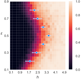
The phase boundary shown in Figure 2 can be determined via a data collapse from plots such as that shown in Figure 3 for $\epsilon=0.5$. To extract the critical magnetic field strength $h_{c}$, we use a scaling function of the same form $N^{1/\nu}(h-h_{c})$ as that for the average adjacent gap ratio $r$. The reduction in noise allows for a more precise determination of the phase boundary for the same number of disorder realizations. From just data for systems up to size $N=18$ (100 disorder realizations) we are able to determine the phase boundary extrapolated to the thermodynamic limit to an accuracy roughly matching the discrepancy between the conventional quantities $r$ and $f$ determined in the numerically much more expensive study [13]. Intuitively, it makes sense that the average adjacent gap ratio does not have the nice averaging properties of the quantity computed by our neural network, as it completely disregards the properties of the eigenstates and only computes one feature of the spectrum. ML, in contrast, figures out a way to objectively determine the phase by directly recognizing non-trivial properties of the eigenstates.

Another interesting feature in which our method differs from average adjacent gap ratio (as well as most other quantities that have been used in exact diagonalization studies so far) is the value of the scaling exponent $\nu$. Our method consistently yields $\nu\approx 1.6$, independent of the energy range and the precise choice of the training data (under the condition that it is sufficient to ensure convergence of the training), while the average adjacent gap ratio yields $\nu\approx 0.9$ [13]. Both exponents violate the (heuristic) Harris criterion, which for one spacial dimension predicts $\nu>2$ [26, 25], but the larger value of our “order parameter” is closer to the predicted value and there is hope that by moving to even larger system sizes, the best data collapse will be obtained with $\nu\approx 2$. This is another indication that our automatically detected “order parameter” suffer less from finite size effects than more traditional quantities. The size of the region in which the network is unsure which label to assigned shrinks during training and eventually converges. It is a natural measure for the broadening of the phase transition due to finite size effects.

Our method has a number of additional desirable properties. The intermediate values of the average adjacent gap ratio do not have a physical meaning, whereas the output of the neural network has an immediate interpretation as to how certain the phase prediction is. The predicted values of $h_{c}$ and the sizes of the plateaus are stable against changing the regions from which the first kind of training data is generated. The average adjacent gap ratio, actually attains the Poisson value at the integrable point at $h=0$ and it moreover fails to capture the transition if one does not restrict to a fixed magnetization sector. Our method does not suffer from either of these two drawbacks.

Importantly, the computational time for training and evaluating the output of the adversarial neural network is almost negligible compared to the time it takes to generate states for mapping out the phase diagram. As much fewer disorder realizations are necessary per point, this yields a huge net gain in computational time. Our approach thus will allow to meaningfully include states from larger system sizes, which can now be generated with state-of-the-art shift invert algorithms [16], into studies of MBL.

We have demonstrated that ML can be used to automate the task of identifying relevant features that most efficiently capture the physics of phase transitions in quantum systems — a formidable task so far reserved for human researchers. Concretely, the competitive process of adversarial domain adaptation, is able to “invent” a new “order parameter” for the MBL phase transition that yields meaningful results from vastly fewer disorder realizations than established methods.

It seems fair to say that the resulting quantity actually captures the essential physics, as the network, once trained, can correctly identify the phase transition not only at different energy densities, but also in similar but distinct models. This is remarkable, since the MBL transition has mostly defied analytical approaches and even the question of what is the best way to delineate the phase could not be resolved in a satisfactory way. Our method is directly applicable to other non-standard critical phenomena beyond MBL and can be used to distinguish multiple phases, even across different classes of models, as long as their Hilbert spaces are compatible [24].

As the automatic feature identification does not rely on a human understanding of the underlying physical processes, our approach has the potential to lead to new insights into poorly understood many-body phenomena such as MBL or topological phases through an analysis of the feature extraction layer. The tools for this are still in their infancy, but evolving at a fast pace.

In future work, we will apply the technique demonstrated here to larger system sizes, hope to gain new insights into whether there are additional thermodynamically stable phases near the MBL phase transition [20, 27], and plan to fully explore the flexibility of the adversarial approach, that allows to suppress the dependence of the output on specific non-universal features.

C. G. acknowledges support by the European Union’s Marie Skłodowska-Curie Individual Fellowships (IF-EF) programme under GA: 700140. We also acknowledge financial support from the European Research Council (CoG QITBOX and AdG OSYRIS), the Axa Chair in Quantum Information Science, Spanish MINECO (FOQUS FIS2013-46768, QIBEQI FIS2016-80773-P and Severo Ochoa Grant No. SEV-2015-0522, FisicaTeAMO FIS2016- 79508-P), EU STREP program EQuaM (FP7/2007-2017, Grant No. 323714), EU grant QUIC (H2020- FETProAct-2014 641122), Fundació Privada Cellex, and Generalitat de Catalunya (Grant No. SGR 874 and 875, and CERCA Programme). P. H. acknowledges that this project has received funding from the European Union’s Horizon 2020 research and innovation programme under the Marie Skłodowska-Curie grant agreement No 665884, as well as by the ‘Severo Ochoa 2016-2019’ program at ICFO (SEV-2015-0522). A. D. is financed by a Cellex-ICFO-MPQ fellowship and by a Juan de la Cierva fellowship (IJCI-2017-33180). We acknowledge a hardware donation by Nvidia Corporation.

References

- [1] E. P. van Nieuwenburg, Y.-H. Liu, S. D. Huber, Nat. Phy. p. 4037 (2017).
- [2] J. Carrasquilla, R. G. Melko, Nat. Phys. 13, 431 (2017).
- [3] K. Ch’ng, J. Carrasquilla, R. G. Melko, E. Khatami, Phys. Rev. X 7, 031038 (2017).
- [4] S. J. Wetzel, Phys. Rev. E 96, 022140 (2017).
- [5] L. Wang, Phys. Rev. B 94, 195105 (2016).
- [6] P. Zhang, H. Shen, H. Zhai, Phys. Rev. Lett. 120 (2018).
- [7] F. Schindler, N. Regnault, T. Neupert, Phys. Rev. B 95, 245134 (2017).
- [8] W. Hu, R. R. P. Singh, R. T. Scalettar, Phys. Rev. E 95, 062122 (2017).
- [9] P. Broecker, F. F. Assaad, S. Trebst, arXiv:1707.00663 (2017).
- [10] D. Basko, I. Aleiner, B. Altshuler, Ann. Phys. (N. Y). 321, 1126 (2006).
- [11] A. Pal, D. A. Huse, Phys. Rev. B, 82, 174411 (2010).
- [12] R. Nandkishore, D. A. Huse, Annu. Rev. Condens. Matter Phys. 6, 15 (2015).
- [13] D. J. Luitz, N. Laflorencie, F. Alet, Phys. Rev. B 91 (2015).
- [14] T. Thiery, F. Huveneers, M. Müller, W. De Roeck, arXiv:1706.09338 (2017).
- [15] S. A. Parameswaran, R. Vasseur, arXiv:1801.07731 (2018).
- [16] F. Pietracaprina, N. Macé, D. J. Luitz, F. Alet, arXiv:1803.05395 (2018).
- [17] D. A. Abanin, E. Altman, I. Bloch, M. Serbyn, arXiv:1804.11065 (2018).
- [18] M. Serbyn, Z. Papić, D. A. Abanin, Phys. Rev. Lett., 111, 127201 (2013).
- [19] D. A. Huse, R. Nandkishore, V. Oganesyan, Phys. Rev. B, 90, 174202 (2014).
- [20] J. A. Kjäll, J. H. Bardarson, F. Pollmann, Phys. Rev. Lett., 113, 107204 (2014).
- [21] T. Enss, F. Andraschko, J. Sirker, Phys. Rev. B 95, 045121 (2017).
- [22] K. Kudo, T. Deguchi, arXiv:1803.06474 (2018).
- [23] Y. Ganin, et al., J. Mach. Learn. Res. 17, 1 (2016).
- [24] P. Huembeli, A. Dauphin, P. Wittek, Phys. Rev. B 97, 134109 (2018).
- [25] A. B. Harris, J. Phys. Cond. Matt., 28, 421006 (2016).
- [26] A. B. Harris, J. Phys. C: Solid State Phys., 7, 1671 (1974).
- [27] J. Goold, C. Gogolin, S. R. Clark, J. Eisert, A. Scardicchio, A. Silva, Phys. Rev. B, 92, 180202(R) (2015).
- [28] N. Srivastava, G. E. Hinton, A. Krizhevsky, I. Sutskever, R. Salakhutdinov, J. Mach. Learn. Res. 15, 1929–1958 (2014).