Physically-Constrained Data-Driven, Filtered Reduced Order Modeling of Fluid Flows
Abstract
In [70], we proposed a data-driven filtered reduced order model (DDF-ROM) framework for the numerical simulation of fluid flows, which can be formally written as
The new DDF-ROM was constructed by using ROM spatial filtering and data-driven ROM closure modeling (for the Correction term) and was successfully tested in the numerical simulation of a 2D channel flow past a circular cylinder at Reynolds numbers and .
In this paper, we propose a physically-constrained DDF-ROM (CDDF-ROM), which aims at improving the physical accuracy of the DDF-ROM. The new physical constraints require that the CDDF-ROM operators satisfy the same type of physical laws (i.e., the nonlinear operator should conserve energy and the ROM closure term should be dissipative) as those satisfied by the fluid flow equations. To implement these physical constraints, in the data-driven modeling step of the DDF-ROM, we replace the unconstrained least squares problem with a constrained least squares problem. We perform a numerical investigation of the new CDDF-ROM and standard DDF-ROM for a 2D channel flow past a circular cylinder at Reynolds numbers and . To this end, we consider a reproductive regime as well as a predictive (i.e., cross-validation) regime in which we use as little as of the original training data. The numerical investigation clearly shows that the new CDDF-ROM is significantly more accurate than the DDF-ROM in both regimes.
keywords
reduced order modeling, data-driven modeling, spatial filter, physical constraintsAMS
65M60, 76F651 Introduction
To present the new reduced order model (ROM), we use the incompressible Navier-Stokes equations (NSE):
| (1) | |||
| (2) |
where is the velocity, the pressure, and the Reynolds number.
We use the initial condition and (for simplicity) homogeneous Dirichlet boundary conditions: .
ROMs have been used to reduce the computational cost of scientific and engineering applications that are governed by relatively few recurrent dominant spatial structures [6, 9, 12, 26, 28, 29, 43, 50, 52, 65].
In an offline stage, full order model (FOM) data on a given time interval are used to build the ROM.
In an online stage, ROMs are repeatedly used for parameter settings and/or time intervals that are different from those used to build them.
For a given general PDE, Projection ROMs (Proj-ROMs) [7, 29, 43] strategy for approximating its solution, , is: (i) Choose a few dominant modes (which represent the recurrent spatial structures) as basis functions. (ii) Replace with in the given PDE. (iii) Use a Galerkin projection of PDE() onto the ROM space to obtain the Proj-ROM. For example, in fluid dynamics, the Proj-ROM often takes the form
| (3) |
where is the vector of unknown ROM coefficients and are ROM operators that are assembled in the offline stage.
Data-Driven ROMs (DD-ROMs) (e.g., sparse identification of nonlinear dynamics [13] and operator inference method [48, 49]) use a fundamentally different strategy: They first postulate a ROM ansatz
| (4) |
and then they choose the operators and to minimize the difference between the FOM and ansatz (4) [14, 34]:
| (5) |
Both Proj-ROMs and DD-ROMs are facing grand challenges: One of the main roadblocks for Proj-ROMs is that they are not accurate models for the dominant modes: In practice, a corrected Proj-ROM is generally used instead [2, 5, 8, 10, 11, 16, 24, 47, 51]:
| (6) |
Thus, the ROM closure problem (i.e., the modeling of the Correction term in (6)) needs to be addressed. DD-ROMs, on the other hand, can be sensitive to noise in the data, since its operators and are obtained from an inverse problem [27, 66].
In [70], we proposed a data-driven filtered ROM (DDF-ROM), which is a hybrid Proj-ROM/DD-ROM framework in which the classical Proj-ROM framework is used to model the linear operators and the DD-ROM framework is used to model the nonlinear operators. Next, we briefly describe the main steps used in the construction of the DDF-ROM. The philosophy employed in the DDF-ROM construction is to use the classical Galerkin method whenever possible (i.e., for the linear operators) and invoke data-driven modeling only when necessary (i.e., for the nonlinear operators). The hybrid character of the new framework is reminiscent of data assimilation [32]: the classical Galerkin method is at the core of the framework, and data-driven modeling is used solely to improve its accuracy.
We build the DDF-ROM framework in two steps. In the first step, we put forth ROM spatial filtering to discover the exact mathematical formula for the Correction term in (6):
| (7) |
In the second step, we utilize data-driven modeling to find a useful approximation for the Correction term in (7). Specifically, we make the ansatz
| (8) |
and choose and to minimize the difference between the Exact Mathematical Formula in (7) and our ansatz (8), both calculated with the available FOM data:
| (9) |
At the end of the two steps, we obtain the DDF-ROM
| (10) |
The DDF-ROM framework solves the Proj-ROM’s closure problem, since the Correction term is modeled by data-driven modeling in (8)–(9). Furthermore, DDF-ROM is more robust to noise than standard DD-ROMs, since DDF-ROM employs data-driven modeling (which is an inverse problem sensitive to noise) only to model the Correction term in (6), whereas the DD-ROMs use it to model all the ROM operators (compare (9) with (5)).
We note that data-driven closure modeling for non-ROM settings is an extremely active research area, see, e.g., [21, 36]. We also note that there are other data-driven ROM closure models, see, e.g., [18, 33, 39, 25, 59, 4, 46]. We emphasize, however, that these data-driven ROM closure models are different from our DDF-ROM:
(i) They do not use spatial filtering (as in LES) to isolate the ROM subfilter-scale stress tensor (i.e., the Correction term);
(iii) They only use the ROM projection to define the Correction term. In contrast, our DDF-ROM framework is general and can accommodate any type of spatial filter. For example, we could use the ROM differential filter, which was shown to outperform the ROM projection in the numerical investigation of ROMs for 3D flow past a cylinder at [69].
In [70], we investigated the DDF-ROM in the numerical simulation of a 2D channel flow past a circular cylinder at Reynolds numbers , and .
The DDF-ROM was significantly more accurate than the standard projection ROM.
Furthermore, the computational costs of the DDF-ROM and the standard projection ROM were similar, both costs being orders of magnitude lower than the computational cost of the full order model.
Although the DDF-ROM yielded good results [70], these results got worse when the ROM dimension was decreased below a certain threshold. To address this issue, we propose the physically constrained DDF-ROM (CDDF-ROM), which aims at improving the physical accuracy of the DDF-ROM. These physical constraints require that the operator in the DDF-ROM (10) be negative semidefinite and the operator be energy conserving (which resembles the constraints satisfied by the operators and ). To implement these physical constraints, we replace the unconstrained least squares problem (9) solved in the data-driven modeling step of the DDF-ROM with a constrained least squares problem.
We note that it has long been known that improving the physical accuracy of a discretization leads to more accurate solutions in all measures, especially over long time intervals.
Thus, physical constraints have been used for decades in the CFD community (see, e.g., Arakawa’s pioneering work [3], as well as more recent developments [1, 17, 22, 37, 53, 64, 58]).
More recently, physical constraints have started to be used in standard (i.e., without ROM) LES closure modeling, see, e.g., [21].
Finally, physical constraints have also been used in standard ROM (i.e., without closure modeling), see, e.g., [38, 31, 55].
To our knowledge, the CDDF-ROM proposed in this paper is the first physically constrained ROM closure model.
The rest of the paper is organized as follows: In Section 2, we review the DDF-ROM proposed in [70]. In Section 3, we propose the new CDDF-ROM. In Section 4, we perform a numerical investigation of the new CDDF-ROM in the numerical simulation of a 2D flow past a circular cylinder at Reynolds numbers , and . Finally, in Section 5, we summarize our findings and outline future research directions.
2 Data-Driven Filtered ROM (DDF-ROM)
In this section, we briefly review the DDF-ROM proposed in [70]. For more details, the reader is referred to [70].
For the ROM basis, we use the proper orthogonal decomposition (POD) [29, 43, 63, 67]. We emphasize, however, that other ROM bases (e.g., the dynamic mode decomposition (DMD) [35, 41, 56, 61]) could be used in the DDF-ROM construction. Given snapshots (e.g., the finite element solutions) of the NSE (1)–(2), the POD space approximates the snapshots optimally with respect to the -norm. The POD approximation of the velocity is defined as
| (11) |
where are the sought time-varying coefficients, which are determined by solving the following system of equations:
| (12) |
In (12), we assume that the modes are perpendicular to the discrete pressure space. Plugging (11) into (12) yields the Galerkin ROM (G-ROM):
| (13) |
which can be written componentwise as follows:
| (14) |
where and .
The DDF-ROM framework is constructed in two steps. In the first step, we propose ROM spatial filtering to discover the exact mathematical formula for the “Correction” in the Proj-ROM (6), which is reminiscent of large eddy simulation (LES) [57]. In this paper, we exclusively use the ROM projection [68, 69] as a spatial filter, but we note that we could also use other spatial filters (e.g., the ROM differential filter [69, 71]).
For a fixed and a given (where is the FE space), the ROM projection [68, 69] seeks such that
| (15) |
Filtering the NSE (see Section 3.2 in [70] for details), we obtain the spatially filtered ROM:
| (16) |
where the ROM stress tensor is
| (17) |
The spatially filtered ROM can be written as:
| (18) |
where and are the same as those in (13) and the components of are given by
| (19) |
The filtered ROM (18) is an -dimensional ODE system for .
Since , the F-ROM (18) is a computationally efficient surrogate model for the FOM (i.e., the FE approximation of the NSE, which is an -dimensional ODE system).
We emphasize, however, that the F-ROM (18) is not a closed system of equations, since the ROM stress tensor (which is used in the definition of ; see (19)) depends on (see (17)).
Thus, to close the F-ROM (18), we need to solve the ROM closure problem [18, 23, 39, 45, 62, 68], i.e., to find a formula .
The explicit formula for (see (17) and (19)), allows for the first time the use of data-driven modeling of the entire missing ROM information.
In the second step of the DDF-ROM construction, we use data-driven modeling to solve the ROM closure problem, i.e., to find a formula in (18). To make the F-ROM (18) resemble the standard G-ROM (13), we make the following ansatz:
| (20) |
Using ansatz (20) in the F-ROM (18) yields a closed system of equations. To find and in (20), we use data-driven modeling. That is, we find and that ensure the highest accuracy of the vector in the filtered ROM (18). To this end, we minimize the -norm of the difference between computed with the FOM data and equations (17) and (19), and computed with the ansatz (20) and the ROM coefficients obtained from the snapshots. Thus, we solve the following optimization problem [44, 49]:
| (21) |
where is the Euclidian norm in and is the true computed from the snapshot data. The optimal and are used in the filtered ROM (18), yielding the data-driven filtered ROM (DDF-ROM)
| (22) |

Remark 2.1 (The Role of the Ansatz in the DDF-ROM: The Ideal DDF-ROM).
The effect of the ansatz (20) on the numerical results (see Section 4 for details) is illustrated in Fig. 1. An “ideal” DDF-ROM (i.e., a DDF-ROM that uses the true ) is almost as accurate as the FOM, even with ! Using the ansatz (and solving the least squares problem) yields results that are qualitatively similar, but loses some of the “ideal” DDF-ROM’s accuracy. (Of course, we note that the “ideal” DDF-ROM is used only for illustration purposes; it is not a practical ROM, since it can only be used with the training data.)
3 Physically Constrained DDF-ROM (CDDF-ROM)
The operators and in the G-ROM (13) satisfy several physical constraints: First, the operator is negative semidefinite:
| (23) |
Second, if one uses the skew-symmetric formulation of the nonlinearity, the operator satisfies
| (24) |
A natural question is whether the DDF-ROM operators and should also satisfy any physical constraints.
We conjecture that the DDF-ROM operators and satisfy physical constraints that are consistent with the physical constraints satisfied by the ROM subfilter-scale stress tensor , which is used in their construction (see equations (17) and (19)). In [19], it was shown that the role of the ROM subfilter-scale stress tensor (i.e., the “Correction” in (6)) is to dissipate energy. Thus, we conjecture that the constraint that we need to enforce in the DDF-ROM construction is
| (25) |
The challenge in enforcing this constraint is that yields quadratic terms, whereas yields cubic terms. Thus, we propose to replace (25) with the following constraints:
| (26) |
which are easier to implement. Furthermore, the constraints (26) resemble the constraints satisfied by the operators and in the G-ROM, i.e., the constraints (23) and (24), respectively. To enforce the first constraint in (26), sufficient conditions are [33]:
| (27) |
and
| (28) |
To enforce the second constraint in (26), sufficient conditions are:
| (29) | |||||
| (30) | |||||
| (31) |
We emphasize that, from the implementation standpoint, enforcing constraints (26) in the data-driven ROM closure modeling is straightforward: Instead of solving the unconstrained least squares problem (21), we just need to solve a constrained least squares problem with constraints (26). Thus, the physically-constrained data-driven filtered ROM (CDDF-ROM) has the form
| (32) |
where the operators and , instead of solving the unconstrained least squares problem (21) (as is done in the DDF-ROM), solve the following constrained least squares problem:
| (33) |
We note that, in data-driven modeling, physical constraints have been enforced in, e.g., [33, 38]. We emphasize, however, that the CDDF-ROM setting is different from that used in [33, 38]: Indeed, in [33, 38] the authors consider pure data-driven ROMs (4), which only involve operators and (without and ). The new DDF-ROM (22), on the other hand, is a hybrid data-driven/projection ROM, so it involves both G-ROM operators ( and ) and data-driven operators ( and ).
4 Numerical Results
In this section, we perform a numerical investigation of the new CDDF-ROM (32)–(33). Specifically, we investigate whether the constrained data-driven modeling in the new CDDF-ROM construction yields more accurate results than the unconstrained data-driven modeling in the DDF-ROM proposed in [70]. To this end, we compare the new CDDF-ROM with the DFF-ROM in the numerical simulation of a 2D flow past a circular cylinder at Reynolds numbers , and [60, 42]. As a benchmark for our comparison, we use the FOM data obtained with a FE simulation. Since most of the numerical investigation in this section is performed for , we present the background material (e.g., computational setting and ROM construction) for this case and only list the main differences from the test case when we consider the higher Reynolds number cases (i.e., and ). The rest of the section is organized as follows: In Section 4.1, we describe the test problem setup. In Section 4.2, we outline the snapshot and ROM generation. In Section 4.3, we discuss the computational efficiency of the new CDDF-ROM. In Section 4.5, we compare the new CDDF-ROM with the DDF-ROM. Finally, in Section 4.6, we present a cross-validation of the two ROMs, i.e., we test the ROMs for data that was not used to train the ROM closure model. Specifically, we investigate the predictive capabilities of the CDDF-ROM.
4.1 Test Problem Setup
The domain is a rectangular channel with a radius= cylinder, centered at , see Figure 2. No slip boundary conditions are prescribed for the walls and on the cylinder, the inflow profile is given by [30, 54] , and appropriate outflow boundary conditions are used. The kinematic viscosity is , there is no forcing, and the flow starts from rest.
4.2 Snapshot and ROM Generation
To compute the snapshots, we use the commonly used linearized BDF2 temporal discretization, together with a FE spatial discretization utilizing the Scott-Vogelius element. On time step , we use a backward Euler temporal discretization. All simulations use a time step size of . We compute until a statistically steady state is reached (which occurs at about ), and then compute to . Snapshots are taken to be the solutions at each time step from to , which corresponds to one period. Thus, in total 166 snapshots were collected. We compute on two different meshes, which provide approximately 103K and 35K velocity degrees of freedom. The 103K mesh gives essentially a fully resolved solution, and the lift and drag predictions agree well with results from fine discretizations in [15, 60]: Results from the 35K meshes are only slightly less accurate. The results for the test case are obtained on the 35K mesh; the results for the and test cases are obtained on the 103K mesh.
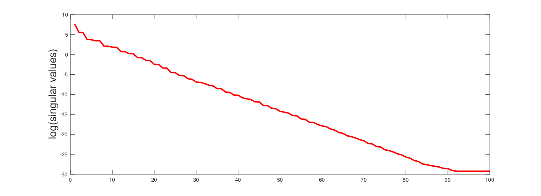
The ROM modes are created from the snapshots in the usual way. The first mode is chosen to be the snapshot average, which satisfies the boundary conditions. This mode is then subtracted from the snapshots, and finally an eigenvalue problem is solved to find the dominant modes of these adjusted snapshots (see [15] for a more detailed description of the process). The singular values of the snapshot matrix are plotted in Figure 3.
With the dominant modes created, the ROM is constructed as discussed in Section 2 using the BDF2 temporal discretization. In all of our tests, just as in the FE simulations, we take ; this choice creates no significant temporal error in any of our simulations (tests were done with varying to verify that 0.002 is sufficiently small). The ROM initial condition at is the projection of the FE solution at into the ROM space. The ROM initial condition at is obtained by using the backward Euler method. The ROMs are run from this initial time (now called ), and continued to . The ROMs are tested using three values: , and .
To allow more flexibility in the computational implementation, instead of using the constraints in (27), we introduce a parameter (which is typically small) and enforce the constraints . To solve the constrained optimization problem, we used MATLAB toolbox lsqlin with interior-point method, where , , and StepTolerance .
4.3 Computational Efficiency
Although the CDDF-ROM and DDF-ROM are more accurate than the G-ROM, the computational cost of calculating and in the offline phase can be significant. Thus, in [70], we proposed the following practical approach for reducing the computational cost of the and calculation: Since , the rank of the snapshot matrix, can be large in practical applications,instead of using to compute the Correction term in (17), we utilized the following approximation:
| (34) |
. In (34), we replaced with and the ROM projection on with the ROM projection on . In practice, the parameter in (34), where , should be chosen to balance accuracy and efficiency in the DDF-ROM [70]. In our numerical investigation, however, we varied the parameter value to achieve the highest level of accuracy.
4.4 Ill-Conditioning
In Section 4 in [70], we observed that the least squares problem used to compute the DDF-ROM operators and was ill-conditioned. We also noted that, in general, data-driven least squares problems can be ill-conditioned; e.g., the least squares problem in the data-driven operator inference method proposed in [49] was also ill-conditioned. To remedy this ill-conditioning, in Algorithm 1 in [70], we used the truncated singular value decomposition (SVD) [20] (see [49] for alternative approaches). The CDDF-ROM’s constrained least squares problem (33) is again ill-conditioned, just as the DDF-ROM’s unconstrained least squares problem. To tackle this ill-conditioning, we use again the truncated SVD procedure (see Step 6 of Algorithm 1 in [70]).
4.5 CDDF-ROM vs DDF-ROM
In this section, we compare the new CDDF-ROM with the DDF-ROM. As a benchmark, we use the FOM. We present results for three Reynolds numbers: , and .
Just as the DDF-ROM, the CDDF-ROM is sensitive to variations in its parameters: (the tolerance used in the truncated-svd algorithm) and (the dimension of the projection space). In addition, CDDF-ROM is also sensitive to , which is the parameter used in the constrained least squares problem in Section 3. In what follows, we present results for the optimal parameter values that were found by trial and error.
4.5.1 Reynolds Number
In this section, we present results for .
First, we consider . We note that is the minimum value for which CDDF-ROM yields accurate results. Lower values yield inaccurate results in our numerical investigation. For the CDDF-ROM, we use ; for the DDF-ROM, we use . The energy evolution in Fig. 4 clearly shows that the CDDF-ROM is dramatically more accurate than the DDF-ROM. The same holds for the drag evolution, although the difference is not as big. Finally, the lift evolution of CDDF-ROM is similar to that of DDF-ROM.


Next, we investigate the case . This time, the minimum value that yields accurate results for CDDF-ROM and DDF-ROM is . For the CDDF-ROM, we use ; for the DDF-ROM, we use . In Fig. 5, we plot the evolution of energy, lift, and drag coefficients for CDDF-ROM, DDF-ROM, and FOM. As in the case, the CDDF-ROM is significantly more accurate than the DDF-ROM.


We conclude that the CDDF-ROM is significantly more accurate than the DDF-ROM for low values, for which the latter does not perform well. We note, however, for higher values for which the DDF-ROM performs well, the CDDF-ROM does not show a visible improvement.
4.5.2 Reynolds Number
In this section, we present results for .
For the test case, to compute the snapshots, we use the same approach as that described in Section 4.2, except that the snapshots are the solutions at each time step from to , which correspond to one period. Thus, in this case we collected a total of snapshots. As ROM initial condition, we use the projection of the snapshot at on the ROM space.
First, we consider ; is the minimum value for which CDDF-ROM yields accurate results. For the CDDF-ROM, we use ; for the DDF-ROM, we use . The energy evolution in Fig. 6 clearly shows that the CDDF-ROM is dramatically more accurate than the DDF-ROM. Since the lift and drag evolutions are similar to those for , in what follows we will not include plots for these quantities.

Next, we investigate the case . Again, the minimum value that yields accurate results for CDDF-ROM and DDF-ROM is . For the CDDF-ROM, we use ; for the DDF-ROM, we use . In Fig. 7, we plot the evolution of energy coefficients for CDDF-ROM, DDF-ROM, and FOM. As in the case, the CDDF-ROM is significantly more accurate than the DDF-ROM.

4.5.3 Reynolds Number
In this section, we present results for .
For the test case, to compute the snapshots, we use the same approach as that described in Section 4.2, except that the snapshots are the solutions at each time step from to , which correspond to one period. Thus, in this case we collected a total of snapshots. As ROM initial condition, we use the projection of the snapshot at on the ROM space.
First, we consider ; is the minimum value for which CDDF-ROM yields accurate results. For the CDDF-ROM, we use ; for the DDF-ROM, we use . The energy evolution in Fig. 8 clearly shows that the CDDF-ROM is dramatically more accurate than the DDF-ROM. The plot at the bottom of Fig. 8 also shows that although the CDDF-ROM energy grows in time, it does so at a slower rate than the DDF-ROM energy.


Next, we investigate the case . This time, the minimum value that yields accurate results for CDDF-ROM and DDF-ROM is . For the CDDF-ROM, we use ; for the DDF-ROM, we use . In Fig. 9, we plot the evolution of energy coefficients for CDDF-ROM, DDF-ROM, and FOM. As in the case, the CDDF-ROM is significantly more accurate than the DDF-ROM.

4.6 CDDF-ROM Cross-Validation: Predictive Investigation
In this section, we perform a cross-validation of the CDDF-ROM. For comparison purposes, we also consider the DDF-ROM. To this end, we test the two ROMs in settings that are different from the setting used to “train” the ROM closure model (i.e., ). That is, we investigate the predictive capabilities of the CDDF-ROM.
We consider two types of predictive investigations, both of which use fewer snapshots than those used in the previous sections:
(i) Equally Spaced Snapshots: For this type of predictive investigation, in the constrained least squares problem (33) used to construct the CDDF-ROM’s operators and , instead of using with spanning an entire period, we used with spanning just of the entire period. The parameter is the number of time steps required to complete a full period and takes the following values: For , for , and .
(ii) Unequally Spaced Snapshots: This type of predictive investigation is similar to the one above. The only difference is that instead of choosing equally spaced snapshots, we use unequally spaced snapshots that are selected from the first part of the period. Thus, the snapshots do not include information from the last part of the period, which makes this predictive investigation sonewhat more challenging than the previous one.
4.6.1 Reynolds Number
In this section, we present results for . We also consider .
First, we consider the case of equally spaced snapshots for , which corresponds to data of an entire period. We note that is the minimum value for which CDDF-ROM yields accurate results. For the CDDF-ROM, we use ; for the DDF-ROM, we use . In Fig. 10, we plot the evolution of energy coefficients. Even for this drastic truncation, the CDDF-ROM performs very well; the DDF-ROM, on the other hand, is very inaccurate.

Next, we consider the case of unequally spaced snapshots collected from the first of the entire period. This time, is the minimum value for which CDDF-ROM yields accurate results. For the CDDF-ROM, we use ; for the DDF-ROM, we use . In Fig. 11, we plot the evolution of energy coefficients. The CDDF-ROM is again dramatically more accurate than DDF-ROM.

4.6.2 Reynolds Number
In this section, we present results for . Again, we consider .
First, we consider the case of equally spaced snapshots for , which corresponds to data of an entire period. We note that is the minimum value for which CDDF-ROM yields accurate results. For the CDDF-ROM, we use ; for the DDF-ROM, we use . In Fig. 12, we plot the evolution of energy coefficients. Even for this drastic truncation, the CDDF-ROM performs very well; the DDF-ROM, on the other hand, is very inaccurate.

Next, we consider the case of unequally spaced snapshots collected from the first of the entire period. This time, is the minimum value for which CDDF-ROM yields accurate results. For the CDDF-ROM, we use ; for the DDF-ROM, we use . In Fig. 13, we plot the evolution of energy coefficients. The CDDF-ROM is again dramatically more accurate than DDF-ROM.

4.6.3 Reynolds Number
In this section, we present results for . This time, we consider , which is the lowest value for which CDDF-ROM yields accurate results.
First, we consider the case of equally spaced snapshots for , which corresponds to data of an entire period. We note that is the minimum value for which CDDF-ROM yields accurate results. For the CDDF-ROM, we use ; for the DDF-ROM, we use . In Fig. 14, we plot the evolution of energy coefficients. Even for this drastic truncation, the CDDF-ROM performs very well; the DDF-ROM, on the other hand, is very inaccurate.

Next, we consider the case of unequally spaced snapshots collected from the first of the entire period. This time, is the minimum value for which CDDF-ROM yields accurate results. For the CDDF-ROM, we use ; for the DDF-ROM, we use . In Fig. 15, we plot the evolution of energy coefficients. The CDDF-ROM is again dramatically more accurate than DDF-ROM.

4.6.4 Parameter Sensitivity
To ensure a fair comparison between the DDF-ROM and CDDF-ROM, for each model we used optimal parameters (i.e., the parameter used in (34) to ensure the CDDF-ROM’s computational efficiency), (i.e., the tolerance value used in the truncated SVD method for the constrained least squares problem), and (i.e., the tolerance used to enforce the constraints in the constrained optimization problem solved with MATLAB toolbox lsqlin with interior-point method; see Section 4.2). Those optimal parameters were selected to ensure that the ROM energy evolution matches best the FOM energy evolution. (This, in turn, ensured the best ROM lift/drag evolutions.)
We note, however, that in our numerical investigation both the DDF-ROM and CDDF-ROM displayed a high sensitivity with respect to the parameters and . This is not surprising, since in Section 5.4 in [70] we showed that the DDF-ROM was sensitive with respect to parameters and . The CDDF-ROM inherits this DDF-ROM’s sensitivity and, in addition, is also sensitive with respect to . In Section 5, we propose methods to alleviate the CDDF-ROM’s sensitivity with respect to these parameters.
5 Conclusions
In this paper, we have proposed a major improvement to the data-driven filtered ROM (DDF-ROM) introduced in [70] by adding physical constraints that increase the DDF-ROM’s physical accuracy. In the new physically-constrained DDF-ROM (CDDF-ROM), the constraints on the data-driven operators are mimicking the physical laws satisfied by the fluid flow equations (i.e., the nonlinear operator should conserve energy and the ROM closure term should be dissipative). Thus, instead of using unconstrained data-driven modeling for the ROM closure problem (which is used in the DDF-ROM construction), we proposed using physically-constrained data-driven modeling. We investigated the new CDDF-ROM in the numerical simulation of a 2D channel flow past a circular cylinder at Reynolds numbers , and . To this end, we compared the CDDF-ROM with the DDF-ROM. As a benchmark, we used the FOM data. The CDDF-ROM was dramatically more accurate than the original DDF-ROM in predicting the evolution of the energy coefficients. It was also more accurate in predicting the evolution of lift and drag coefficients, although the improvement was not as large. Finally, we performed a cross-validation of the CDDF-ROM by testing it, together with the standard DDF-ROM, on data that was not used to train the ROM closure model; that is, we investigated the predictive capabilities of the CDDF-ROM. To this end, we considered two types of cross-validations: (i) with equally spaced snapshots, in which we considered as few as of the original set of snapshots; and (ii) with unequally spaced snapshots, in which we considered as few as of the first snapshots in the original set. For both types of cross-validations, the CDDF-ROM dramatically outperformed the original DDF-ROM. This numerical investigation in the reproductive and predictive regimes clearly showed that the physically-constrained CDDF-ROM is significantly more accurate than the DDF-ROM.
We plan to investigate several research avenues: Probably the most important research direction is the further investigation of the CDDF-ROM’s sensitivity with respect to the parameters used to solve the constrained least squares problem. We plan to investigate alternative means of treating the ill-conditioning of the CDDF-ROM’s constrained least squares problem (see, e.g., the approach used in [49], where the authors combined trajectories of different initial conditions to decrease the ill-conditioning of their data-driven least squares problem). Furthermore, we plan to investigate whether there is any connection between the ill-conditioning of the CDDF-ROM’s constrained least squares problem and overfitting. If such a connection exists, we plan to investigate methods that mitigate overfitting [13, 38, 40]. These alternative methods could eliminate altogether the need for the parameter used in the CDDF-ROM’s truncated SVD algorithm or yield numerical algorithms with lower parameter sensitivity.
Another potential research avenue is the investigation of weaker constraints in the CDDF-ROM’s constrained least squares problem. For example, since the constraints (27)–(31) are sufficient but not necessary conditions to satisfy the general constraint (26), we plan to investigate weaker constraints that satisfy the general constraint (26). We will also investigate alternative models that impose the constraint (25) in a statistical sense, not pointwise, as is done in this paper. These alternative, weaker constraints might decrease the ill-conditioning of CDDF-ROM’s constrained least squares problem, which in turn could yield numerical algorithms with lower parameter sensitivity.
References
- [1] R. V. Abramov and A. J. Majda, Discrete approximations with additional conserved quantities: deterministic and statistical behavior, Methods Appl. Anal., 10 (2003), pp. 151–190.
- [2] D. Amsallem and C. Farhat, Stabilization of projection-based reduced-order models, Int. J. Num. Meth. Eng., 91 (2012), pp. 358–377.
- [3] A. Arakawa, Computational design for long-term numerical integration of the equations of fluid motion: Two dimensional incompressible flow, Part I, J. Comput. Phys., 1 (1966), pp. 119–143.
- [4] J. Baiges, R. Codina, and S. Idelsohn, Reduced-order subscales for POD models, Comput. Methods Appl. Mech. Engrg., 291 (2015), pp. 173–196.
- [5] M. J. Balajewicz, E. H. Dowell, and B. R. Noack, Low-dimensional modelling of high-Reynolds-number shear flows incorporating constraints from the Navier–Stokes equation, J. Fluid Mech., 729 (2013), pp. 285–308.
- [6] F. Ballarin, E. Faggiano, S. Ippolito, A. Manzoni, A. Quarteroni, G. Rozza, and R. Scrofani, Fast simulations of patient-specific haemodynamics of coronary artery bypass grafts based on a POD–Galerkin method and a vascular shape parametrization, J. Comput. Phys., 315 (2016), pp. 609–628.
- [7] F. Ballarin, A. Manzoni, A. Quarteroni, and G. Rozza, Supremizer stabilization of POD–Galerkin approximation of parametrized steady incompressible Navier–Stokes equations, Int. J. Numer. Meth. Engng., 102 (2015), pp. 1136–1161.
- [8] M. F. Barone, I. Kalashnikova, D. J. Segalman, and H. K. Thornquist, Stable Galerkin reduced order models for linearized compressible flow, J. Comput. Phys., 228 (2009), pp. 1932–1946.
- [9] P. Benner, S. Gugercin, and K. Willcox, A survey of projection-based model reduction methods for parametric dynamical systems, SIAM Rev., 57 (2015), pp. 483–531.
- [10] M. Benosman, J. Borggaard, O. San, and B. Kramer, Learning-based robust stabilization for reduced-order models of 2D and 3D Boussinesq equations, Appl. Math. Model., 49 (2017), pp. 162–181.
- [11] M. Bergmann, C. H. Bruneau, and A. Iollo, Enablers for robust POD models, J. Comput. Phys., 228 (2009), pp. 516–538.
- [12] D. A. Bistrian and I. M. Navon, An improved algorithm for the shallow water equations model reduction: Dynamic mode decomposition vs POD, Int. J. Num. Meth. Fluids, 78 (2015), pp. 552–580.
- [13] S. L. Brunton, J. L. Proctor, and J. N. Kutz, Discovering governing equations from data by sparse identification of nonlinear dynamical systems, Proc. Natl. Acad. Sci., 113 (2016), pp. 3932–3937.
- [14] D. G. Cacuci, I. M. Navon, and M. Ionescu-Bujor, Computational Methods for Data Evaluation and Assimilation, CRC Press, 2013.
- [15] A. Caiazzo, T. Iliescu, V. John, and S. Schyschlowa, A numerical investigation of velocity-pressure reduced order models for incompressible flows, J. Comput. Phys., 259 (2014), pp. 598–616.
- [16] K. Carlberg, M. Barone, and H. Antil, Galerkin v. least-squares Petrov–Galerkin projection in nonlinear model reduction, J. Comput. Phys., 330 (2017), pp. 693–734.
- [17] M. Case, A. Labovsky, L. Rebholz, and N. Wilson, A high physical accuracy method for incompressible magnetohydrodynamics, Int. J. Numer. Anal. Mod., Series B, 1 (2010), pp. 219–238.
- [18] M. D. Chekroun, H. Liu, J. C. McWilliams, and S. Wang, Markovian and non-Markovian closures for stochastic partial differential equations, In preparation, (2017).
- [19] M. Couplet, P. Sagaut, and C. Basdevant, Intermodal energy transfers in a proper orthogonal decomposition–Galerkin representation of a turbulent separated flow, J. Fluid Mech., 491 (2003), pp. 275–284.
- [20] J. W. Demmel, Applied Numerical Linear Algebra, Society for Industrial and Applied Mathematics Philadelphia, 1997.
- [21] K. Duraisamy, G. Iaccarino, and H. Xiao, Turbulence modeling in the age of data, arXiv preprint, http://arxiv.org/abs/arXiv:1804.00183, (2018).
- [22] G. Fix, Finite element models for ocean circulation problems, SIAM J. Appl. Math., 29 (1975), pp. 371–387.
- [23] B. Galletti, A. Bottaro, C.-H. Bruneau, and A. Iollo, Accurate model reduction of transient and forced wakes, Eur. J. Mech. B-Fluid., 26 (2007), pp. 354–366.
- [24] S. Giere, T. Iliescu, V. John, and D. Wells, SUPG reduced order models for convection-dominated convection-diffusion-reaction equations, Comput. Methods Appl. Mech. Engrg., 289 (2015), pp. 454–474.
- [25] A. Gouasmi, E. J. Parish, and K. Duraisamy, A priori estimation of memory effects in reduced-order models of nonlinear systems using the Mori–Zwanzig formalism, Proc. R. Soc. A, 473 (2017), p. 20170385.
- [26] M. Gunzburger, N. Jiang, and M. Schneier, An ensemble-proper orthogonal decomposition method for the nonstationary Navier-Stokes equations, SIAM J. Numer. Anal., 55 (2017), pp. 286–304.
- [27] P. C. Hansen, Discrete Inverse Problems: Insight and Algorithms, vol. 7, Society for Industrial and Applied Mathematics, 2010.
- [28] J. S. Hesthaven, G. Rozza, and B. Stamm, Certified Reduced Basis Methods for Parametrized Partial Differential Equations, Springer, 2015.
- [29] P. Holmes, J. L. Lumley, and G. Berkooz, Turbulence, Coherent Structures, Dynamical Systems and Symmetry, Cambridge, 1996.
- [30] V. John, Reference values for drag and lift of a two dimensional time-dependent flow around a cylinder, Int. J. Num. Meth. Fluids, 44 (2004), pp. 777–788.
- [31] I. Kalashnikova and M. F. Barone, On the stability and convergence of a Galerkin reduced order model (ROM) of compressible flow with solid wall and far-field boundary treatment, Int. J. Num. Meth. Eng., 83 (2010), pp. 1345–1375.
- [32] E. Kalnay, Atmospheric modeling, data assimilation, and predictability, Cambridge Univ Pr, 2003.
- [33] D. Kondrashov, M. D. Chekroun, and M. Ghil, Data-driven non-Markovian closure models, Phys. D, 297 (2015), pp. 33–55.
- [34] J. N. Kutz, Data-driven Modeling & Scientific Computation: Methods for Complex Systems & Big Data, Oxford University Press, 2013.
- [35] J. N. Kutz, S. L. Brunton, B. W. Brunton, and J. L. Proctor, Dynamic Mode Decomposition: Data-Driven Modeling of Complex Systems, SIAM, 2016.
- [36] J. Ling, R. Jones, and J. Templeton, Machine learning strategies for systems with invariance properties, J. Comput. Phys., 318 (2016), pp. 22–35.
- [37] J.-G. Liu and W. Wang, Energy and helicity preserving schemes for hydro and magnetohydro-dynamics flows with symmetry, J. Comput. Phys., 200 (2004), pp. 8–33.
- [38] J.-C. Loiseau and S. L. Brunton, Constrained sparse Galerkin regression, J. Fluid Mech., 838 (2018), pp. 42–67.
- [39] F. Lu, K. K. Lin, and A. J. Chorin, Data-based stochastic model reduction for the Kuramoto–Sivashinsky equation, Phys. D, 340 (2017), pp. 46–57.
- [40] R. Maulik and O. San, A neural network approach for the blind deconvolution of turbulent flows, J. Fluid Mech., 831 (2017), pp. 151–181.
- [41] I. Mezić, Spectral properties of dynamical systems, model reduction and decompositions, Nonlinear Dyn., 41 (2005), pp. 309–325.
- [42] M. Mohebujjaman, L. G. Rebholz, X. Xie, and T. Iliescu, Energy balance and mass conservation in reduced order models of fluid flows, J. Comput. Phys., 346 (2017), pp. 262–277.
- [43] B. R. Noack, M. Morzynski, and G. Tadmor, Reduced-Order Modelling for Flow Control, vol. 528, Springer Verlag, 2011.
- [44] B. R. Noack, P. Papas, and P. A. Monkewitz, The need for a pressure-term representation in empirical Galerkin models of incompressible shear flows, J. Fluid Mech., 523 (2005), pp. 339–365.
- [45] B. R. Noack, M. Schlegel, B. Ahlborn, G. Mutschke, M. Morzynski, P. Comte, and G. Tadmor, A finite-time thermodynamics of unsteady fluid flows, J. Non-Equil. Thermody., 33 (2008), pp. 103–148.
- [46] A. A. Oberai and J. Jagalur-Mohan, Approximate optimal projection for reduced-order models, Int. J. Num. Meth. Engng., 105 (2016), pp. 63–80.
- [47] J. Östh, B. R. Noack, S. Krajnović, D. Barros, and J. Borée, On the need for a nonlinear subscale turbulence term in POD models as exemplified for a high-Reynolds-number flow over an Ahmed body, J. Fluid Mech., 747 (2014), pp. 518–544.
- [48] B. Peherstorfer and K. Willcox, Dynamic data-driven reduced-order models, Comput. Methods Appl. Mech. Engrg., 291 (2015), pp. 21–41.
- [49] B. Peherstorfer and K. Willcox, Data-driven operator inference for nonintrusive projection-based model reduction, Comput. Methods Appl. Mech. Engrg., 306 (2016), pp. 196–215.
- [50] S. Perotto, A. Reali, P. Rusconi, and A. Veneziani, HIGAMod: A Hierarchical IsoGeometric Approach for MODel reduction in curved pipes, Comput. & Fluids, 142 (2017), pp. 21–29.
- [51] B. Protas, B. R. Noack, and J. Östh, Optimal nonlinear eddy viscosity in Galerkin models of turbulent flows, J. Fluid Mech., 766 (2015), pp. 337–367.
- [52] A. Quarteroni, A. Manzoni, and F. Negri, Reduced Basis Methods for Partial Differential Equations: An Introduction, vol. 92, Springer, 2015.
- [53] L. Rebholz, An energy- and helicity-conserving finite element scheme for the Navier-Stokes equations, SIAM J. Numer. Anal., 45 (2007), pp. 1622–1638.
- [54] L. Rebholz and M. Xiao, Improved accuracy in algebraic splitting methods for Navier-Stokes equations, SIAM J. Sci. Comput., 39 (2017), pp. A1489–A1513.
- [55] C. W. Rowley, T. Colonius, and R. M. Murray, Model reduction for compressible flows using POD and Galerkin projection, Phys. D, 189 (2004), pp. 115–129.
- [56] C. W. Rowley, I. Mezić, S. Bagheri, P. Schlatter, and D. S. Henningson, Spectral analysis of nonlinear flows, J. Fluid Mech., 641 (2009), pp. 115–127.
- [57] P. Sagaut, Large Eddy Simulation for Incompressible Flows, Scientific Computation, Springer-Verlag, Berlin, third ed., 2006.
- [58] R. Salmon and L. D. Talley, Generalizations of Arakawa’s Jacobian, J. Comput. Phys., 83 (1989), pp. 247–259.
- [59] O. San and R. Maulik, Neural network closures for nonlinear model order reduction, Adv. Comput. Math., DOI:10.1007/s10444-018-9590-z (2018).
- [60] M. Schfer and S. Turek, The benchmark problem ‘flow around a cylinder’ flow simulation with high performance computers II, in E.H. Hirschel (Ed.), Notes on Numerical Fluid Mechanics, 52, Braunschweig, Vieweg (1996), pp. 547–566.
- [61] P. J. Schmid, Dynamic mode decomposition of numerical and experimental data, J. Fluid Mech., 656 (2010), pp. 5–28.
- [62] S. Sirisup and G. E. Karniadakis, A spectral viscosity method for correcting the long-term behavior of POD models, J. Comput. Phys., 194 (2004), pp. 92–116.
- [63] L. Sirovich, Turbulence and the dynamics of coherent structures. Parts I–III, Quart. Appl. Math., 45 (1987), pp. 561–590.
- [64] C. Sorgentone, S. L. Cognata, and J. Nordstrom, A new high order energy and enstrophy conserving Arakawa-like Jacobian differential operator, J. Comput. Phys., 301 (2015), pp. 167–177.
- [65] R. Ştefănescu, A. Sandu, and I. M. Navon, POD/DEIM reduced-order strategies for efficient four dimensional variational data assimilation, J. Comput. Phys., 295 (2015), pp. 569–595.
- [66] C. R. Vogel, Computational Methods for Inverse Problems, vol. 23, Society for Industrial and Applied Mathematics (SIAM), 2002.
- [67] S. Volkwein, Proper orthogonal decomposition: Theory and reduced-order modelling, Lecture Notes, University of Konstanz, (2013). http://www.math.uni-konstanz.de/numerik/personen/volkwein/teaching/POD-Book.pdf.
- [68] Z. Wang, I. Akhtar, J. Borggaard, and T. Iliescu, Proper orthogonal decomposition closure models for turbulent flows: A numerical comparison, Comput. Meth. Appl. Mech. Eng., 237-240 (2012), pp. 10–26.
- [69] D. Wells, Z. Wang, X. Xie, and T. Iliescu, An evolve-then-filter regularized reduced order model for convection-dominated flows, Int. J. Num. Meth. Fluids, 84 (2017), pp. 598––615.
- [70] X. Xie, M. Mohebujjaman, L. G. Rebholz, and T. Iliescu, Data-driven filtered reduced order modeling of fluid flows, SIAM J. Sci. Comput., (2018). To appear, also available as arXiv preprint, http://arxiv.org/abs/1709.04362.
- [71] X. Xie, D. Wells, Z. Wang, and T. Iliescu, Approximate deconvolution reduced order modeling, Comput. Methods Appl. Mech. Engrg., 313 (2017), pp. 512–534.