An irrational-slope Thompson’s groupThanks: The first author thanks the Spanish Ministry MICINN through grant MTM2017-82740-P for their support. The second and third author were supported by the Royal Society International Exchanges grant IES\R3\170086.

Thompson’s groups were introduced in the 1960s and soon captured the interest of group theorists for their interesting properties. They have spawned a family of groups that have properties similar to the original Thompson’s groups $F$, $T$ and $V$, but each of which is interesting in its own right. The purpose of this paper is to study one of these groups, namely, the group $F_{\tau}$ of piecewise linear homeomorphisms of $[0,1]$ having breakpoints in $\mathbb{Z}[\tau]$ and slopes that are powers of $\tau$, where $\tau$ is the golden ratio $(\sqrt{5}-1)/2$. The group $F_{\tau},$ although having irrational breakpoints, does share many of the properties of the original Thompson’s group $F.$

The group $F_{\tau}$ was introduced by Sean Cleary in [11], where it is first described and proved to be of type $F_{\infty}$. The group $F_{\tau}=G([0,1];\mathbb{Z}[\tau],\langle\tau\rangle)$ is also mentioned in the Bieri-Strebel notes [1], although finite presentations there are only given for groups with rational slopes [1, D.15.10].

After defining the group we devote a section to the combinatorial structure of the group which stems from the representation of elements by pairs of finite rooted trees.

In Section 4 a presentation is obtained:

Theorem 4.4

This infinite presentation can easily be reduced to a finite presentation which is also given.

The subsequent two sections describe the abelianisation of $F_{\tau}$, the commutator subgroup, and the main simplicity result.

Theorem 6.4 The group $F_{\tau}^{\prime}$ is simple.

In Section 7 we present an explicit normal form for the elements of the group:

Theorem 7.3 Each element of $F_{\tau}$ has a unique normal form representative.

As with $F$, the unique normal form is closely related to a unique reduced tree diagram for the element, but here we need a new condition on the normal form to account for possible cancellations which can occur after performing a basic move (as introduced in Section 2).

The final two sections deal with metric considerations. As happens with $F$, the metric on the group can be approximated by the number of carets in the unique reduced tree pair diagram. This gives us quasi-isometric embeddings, into $F_{\tau},$ of some natural copies of $F$.

The reader is assumed to have some familiarity with Thompson’s group $F$. Many of the arguments for $F_{\tau}$ will be similar to those for $F$. In order to avoid repetitions and making this paper unnecessarily long, we will refer to the corresponding constructions and results for $F$ when necessary. A good introduction for $F$, which contains many results which apply here, can be found in [10].

Let $\tau$ be the small golden ratio $\frac{\sqrt{5}-1}{2}=0.6180339887...$, which is a zero of the polynomial $X^{2}+X-1$. We will consider the ring $\mathbb{Z}[\tau]$ of elements of the type $a+b\tau$, where $a$ and $b$ are integers. Observe that $\tau=(1+\tau)^{-1}$ is a unit of this ring, hence we can consider the group $G([0,1];\mathbb{Z}[\tau],\left<\tau\right>)$ of piecewise linear orientation preserving homeomorphisms of $[0,1]$ having breakpoints in the ring $\mathbb{Z}[\tau]$ and slopes in the subgroup $\langle\tau\rangle$ of units of this ring. Groups like these were introduced by Bieri and Strebel [1]. Following Cleary, [11], we denote this group $F_{\tau}$. Cleary proved that the group is of type $F_{\infty}$, so in particular, it is finitely presented, however no explicit finite presentation was given [11]. Cleary also describes a combinatorial structure for $F_{\tau}$, which we are going to develop here, since it will be used extensively throughout this paper.

Observe that, since $1=\tau+\tau^{2}$, the unit interval can be subdivided into two subintervals of lengths $\tau$ and $\tau^{2}$ respectively and this can be done in two ways: $[0,1]=[0,\tau]\cup[\tau,1]$ and $[0,1]=[0,\tau^{2}]\cup[\tau^{2},1]$. Since we also have that $\tau^{k}=\tau^{k+1}+\tau^{k+2}$ (for all $k\geq 0$), each subinterval can be further subdivided into intervals whose lengths are powers of $\tau$. Elements of $F_{\tau}$ are now given by a pair of such subdivisions into $n$ intervals each, together with an order preserving bijection, see [11].

This opens the door to a combinatorial approach to $F_{\tau}$ using binary rooted trees, with a caret representing a subdivision, in a very similar fashion to Thompson’s group $F$. The difficulty here is that we will need two types of carets, since intervals can be subdivided in two ways. Hence subdivisions will be represented by a caret with two edges of different lengths. In Figure 1 we have the two subdivisions of the unit interval given above, represented by their respective carets. An example of an iterated subdivision with its corresponding tree is given in Figure 2.

The reason for representing the shorter subinterval by the longer edge in the caret is that then the nodes in the tree are organised by levels according to the lengths of the corresponding subintervals. A node at level $k$ corresponds to an interval of length $\tau^{k}$. In this way the tree carries more information than just the combinatorial structure of the intervals. See Figure 2 for an example.

The reason for this nomenclature will be apparent later, when we give a presentation of $F_{\tau}.$

An interesting feature of this group is that there are subdivisions which correspond to more than one tree. The simplest example of this phenomenon is the subdivision of the unit interval into three subintervals of lengths $\tau^{2},\tau^{3},\tau^{2}$ given by $[0,\tau^{2}]\cup[\tau^{2},\tau]\cup[\tau,1]$. This can be represented by two trees, one with two $x$-carets and one with two $y$-carets, as shown in Figure 3. In Section 6 we produce a special unique tree pair diagram for each element of $F_{\tau}.$

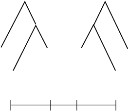
The two trees in Figure 3 are crucial in what is to come. They are completely interchangeable when appearing, even as subtrees, as they represent the same subdivision of an interval. We call the process of interchanging these two configurations inside a tree a basic move. In Figure 4 we illustrate a basic move, represented by the thick lines, on the tree of Figure 2.

Clearly, an element can be represented by more than one tree pair diagram. Besides the usual phenomenon, familiar from $F$, where one can add or remove so-called redundant carets to obtain different tree pairs that represent the same element, here we can have two reduced diagrams representing the same element. Recall that a reduced tree pair diagram is one without redundant carets. An example is given in Figure 5, where a basic move on the right-hand-side diagram will produce redundant carets that can be removed to give the tree pair on the left.

Basic moves are crucial for working with the trees arising for this group. In particular, to be able to understand multiplication of elements via tree pair diagrams. We begin by proving some important properties.

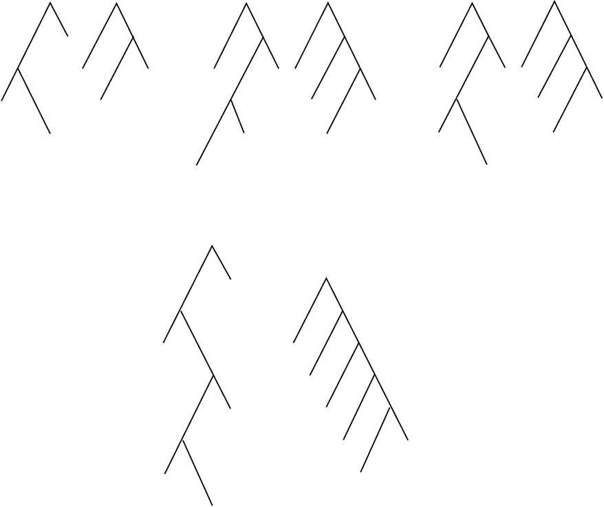
Proof. If the caret to be switched can have a basic move performed on it, then that switches the type. Suppose now that the short edge of this caret ends in a leaf (i.e., has no child), then add a caret of the same type to enable a basic move (see picture 2 of Figure 8). Finally, if the child caret on the short side is of the opposite type, then keep going down short edges until a basic move can be performed. Should this process not result in a basic move, add a caret to the bottom short edge. Then one can perform multiple basic moves going back up to the caret to be switched. See pictures 3, 4 and 5 on Figure 8. $\sqcup$$\sqcap$

The usefulness of basic moves is further illustrated by the following result, which will be used when deriving a presentation in Section 4.

Proof. Let $T_{1}$ and $T_{2}$ be two trees which represent the same subdivision, and assume that their root carets are different. Assume that $T_{1}$ has an $x$-type root caret and $T_{2}$ has a $y$-type root caret. Since $T_{2}$ has a $y$-caret at its root, the common subdivision has a break at the point $\tau$ in the interval. This means that at $T_{1}$, the right edge (which is short) needs to be subdivided further, because we need the break at $\tau$ on $T_{1}$ too. We are going to show that in order for the break at $\tau$ to show up in $T_{1}$, there have to be two consecutive carets of the same type somewhere on $T_{1}$. It follows that a basic move can be performed and the root caret of $T_{1}$ can be switched.

If the right child of the root caret in $T_{1}$ is of $x$-type, then we have two consecutive carets of the same type and a basic move could be performed at the root. Assume then that the short edge of the $x$-type root has a $y$-caret as child. Then the breaks are at the points $\tau^{2}$ and $2\tau^{2}=1-\tau^{3}$. Since $\tau^{2}<\tau<1-\tau^{3}$, the desired breakpoint still has not been produced, see Figure 7.

The tree $T_{1}$ is therefore further subdivided. The point of the proof is that it is necessary to have two consecutive subdivisions of the same type ($x$- or $y$- depending on the parity) to obtain a break at $\tau$. This is because of the following equalities (for even $n$, the odd case is similar):

The odd power can only be produced with two consecutive carets of the same type, see Figure 6.

If below the short edge of the root caret the subsequent carets on their short edges are of alternating the type, we never reach the value $\tau$ because of the strict inequalities:

We would need infinitely many children to obtain a break at $\tau$ corresponding to the equalities

Figure 7 illustrated this fact.

Since the trees are finite, in one of the trees there must be two consecutive carets of the same type, and the root caret can be switched by a sequence of basic moves without adding an extra caret. Therefore we can keep going down the tree switching types of all the carets of different type, adding nothing, until the two trees are exactly the same. $\sqcup$$\sqcap$

As in $F$, multiplication in $F_{\tau}$ is given by composition of maps. To be able to multiply two elements given by tree pairs, we find a common expansion for the target tree of the first element and the source tree of the second element. Consider two elements given by tree pairs $(T_{1},T_{2})$ and $(S_{1},S_{2})$. If it happens that $T_{2}=S_{1}$, then the product will be represented by $(T_{1},S_{2})$. If $T_{1}\neq T_{2}$ we apply the following proposition:

Proof. If the carets are all of the same type, this can be done by just adding carets to construct the least common expansion in the same way as is done with $F$. If both caret types are present we first need to switch the carets in $T$ to agree with those in $T^{\prime}.$ This is done by applying Proposition 2.1, see Figure 8 for an illustration. Once this process is finished we might need to add some more carets to obatin the tree $T^{\prime\prime},$ which is an expansion of $T$ and has $T^{\prime}$ as subtree. $\sqcup$$\sqcap$

This procedure finishes the construction of the algorithm to perform the multiplication of two elements given by two tree pairs $(T_{1},T_{2})$ and $(S_{1},S_{2})$. Find the tree $T_{3}$ which is the common subdivision for $T_{2}$ and $S_{1}$, and find two tree pairs which represent the same elements which look like $(T_{1}^{\prime},T_{3})$ and $(T_{3},S_{2}^{\prime})$. This is done by adding to $T_{1}$ the carets corresponding to those we have added to $T_{2}$, and similarly for the other pair. Finally, the product is given by $(T_{1}^{\prime},S_{2}^{\prime})$. See Figure 9 for a simple example.

To find generators for $F_{\tau}$ we follow the ideas used for $F$. The infinite generating set for $F$ has generators, which are given by binary tree pairs $(T,S)$, where $S$ is a tree where each caret has only right children, also called a spine, and where $T$ is a spine with one additional caret at the bottom left hand leaf. Since for $F_{\tau}$ we have two different kinds of carets, there is ambiguity in this construction. However, by Lemma 2.1, the type of a caret can always be switched. Hence we chose one caret type for the trees we will call spines.

Generators for $F_{\tau}$ will have a spine to which an extra caret is added at the end, as a left child on the source tree, and as a right child on the target one.

Observe from Figure 11 that the key caret is of type $x$ for the generators $x_{n}$ and of type $y$ for $y_{n}$, and this is the reason the carets are named in this way. However, in both cases, the spines have only $x$-carets.

Our goal is to prove that the set of $x_{n}$ and $y_{n}$, for $n\geq 0$, is a generating set for $F_{\tau}$. In a similar fashion to that for $F$, if the target tree of an element is a spine, this element is the product of generators (without taking inverses). In Figure 12 we can see an example of an element which is the product of three generators, obtaining a pair made of a tree and a spine.

In Figure 13 we see why any element given by a tree and a spine can be written as a product of the generators $x_{n}$ and $y_{n}$. If we multiply an element with a spine as a target tree by the generator $x_{i}$ or $y_{i}$, then the result is to attach a caret of the corresponding type to the $i$-th leaf. In this way we can construct a tree paired with a spine. Observe though that the tree constructed this way will always have in the right-hand side all carets of the $x$-type.

Using this construction we can prove:

Proof. Take any element of $F_{\tau}$ given as a pair $(T_{1},T_{2})$ of trees. Using Lemma 2.1 we can assume that we have a spine down the right hand side of each tree. If the trees have an $y$-caret in the right-hand side, use the lemma to change the type of these carets, at the price of adding carets to the trees. The result will be a pair of trees whose right-hand sides have only $x$-carets.

Now, put a spine $S$ in between the two trees. The first tree pair $(T_{1},S)$ gives an element which, by the construction specified above, is the product of generators $x_{n}$ or $y_{n}$. The second pair $(S,T_{2})$ is the inverse of an element also of this type. Hence, any element is a product of the generators $x_{n}$ or $y_{n}$ and their inverses. $\sqcup$$\sqcap$

It is not hard to see that there are some relations which are satisfied by these generators. The combinatorics of the carets, similar to those of $F$, give the following four sets of relators:

1. (1)

   $x_{j}x_{i}=x_{i}x_{j+1}$

2. (2)

   $x_{j}y_{i}=y_{i}x_{j+1}$

3. (3)

   $y_{j}x_{i}=x_{i}y_{j+1}$

4. (4)

   $y_{j}y_{i}=y_{i}y_{j+1}$

where in all cases we have $i<j$. Another set of relators is given by the subdivision which admits two expressions as carets. These relations are $y_{n}^{2}=x_{n}x_{n+1}$. The goal of the next theorem is to show that these are all relations needed to obtain a presentation for $F_{\tau}$.

Proof: Given a word in the generators $x_{i},y_{i}$ which gives the identity, when we construct its corresponding tree pair diagram, the two trees necessarily give rise to the same subdivision. Also, the two trees will have a spine (all $x$-carets) in their right hand sides. According to Proposition 2.2, we can go from one to the other by applying basic moves to one of them, and in this case, the basic moves are never performed on a vertex on the right hand side of the tree. Observe that each basic move corresponds exactly to multiplying our word by a conjugate of relation (5), noting that all instances of relation (5) have spines and hence are precisely those that we need. Hence, using relation (5) we can obtain a word which yields a diagram where the two trees are the same. In the same way as is done for Thompson’s group $F$, this diagram can be seen to be a consequence of relations of the type (1) to (4). Hence, the original word is a consequence of the relations (1) to (5). $\sqcup$$\sqcap$

This presentation allows us to establish a correspondence between tree pair diagrams and a particular type of words. This correspondence is completely analogous to that in Thompson’s group $F$, based on leaf exponents. See [10, Theorem 2.5] or [8, Section 3.1]. Observe that the relations (1)–(4) allow for the ordering of the generators in a word by index, increasing for positive powers and decreasing for negative powers. We have the following result.

This is analogous to the normal form for Thompson’s group $F$. This expression for an element corresponds to its tree pair diagram using leaf exponents. The only difference between $F_{\tau}$ and $F$ is that we can alternate generators $x_{i}$ and $y_{i}$ within the same index, as in the example at Figure 12, where we consider the element $y_{0}x_{1}y_{1}$.

It is not difficult to deduce a finite presentation from the infinite one. From the relations (1)–(4) it is easily seen that the generators with index 2 or higher are conjugates of those with index 1. Hence, the only generators needed are $x_{0},x_{1},y_{0},y_{1}$. Similarly, for each family of relators (1) to (4), only two are needed as happens in Thompson’s group $F$, see, for instance, [10]. For the family (5), observe that if $i\geq 2$, the relation $y_{i}^{2}=x_{i}x_{i+1}$ is a conjugate (by the appropriate power of $x_{0}$) of $y_{1}^{2}=x_{1}x_{2}$. Hence, the following relations are sufficient:

We do not claim that this presentation is optimal, and it is possible that there is a presentation with fewer generators or with fewer relations.

Once we have a presentation, it is easy to abelianise the group. The abelianised group has four generators $\bar{x}_{0},\bar{x}_{1},\bar{y}_{0},\bar{y}_{1}$, and observe that the relations (1)-(4) abelianise trivially. Hence the quotient abelian group has two relations, namely

where we have changed to additive notation for the abelian group. Using the first relation we can eliminate the generator $\bar{x}_{0}$. Defining $\bar{z}=\bar{x}_{1}-\bar{y}_{1}$, the abelianisation can be generated by $\bar{x}_{1},\bar{y}_{0},\bar{z}$ subject to the relation $2\bar{z}=0$. The abelianisation is therefore isomorphic to $\mathbb{Z}^{2}\oplus\mathbb{Z}_{2}$.

The commutator subgroup, that is the kernel of the abelianisation map, can also be completely understood. Looking at the generators $\bar{x}_{1}$ and $\bar{y}_{0}$, we see that they represent the slopes at 0 and at 1, in the same way as holds for Thompson’s group $F$. The map from $F_{\tau}$ to $\mathbb{Z}^{2}$ given by the two components of the abelianisation map generated by $\bar{x}_{1}$ and $\bar{y}_{0}$ coincides (up to a change of basis in $\mathbb{Z}^{2}$) with the map that sends every element to the slopes at 0 and 1.

Observe then that the commutator subgroup is contained in $F_{\tau}^{c}$. However, from the $\mathbb{Z}_{2}$ component we see that it is not equal to it. To describe it clearly, let $z=x_{1}y_{1}^{-1}$, and observe that $z$ maps to $\bar{z}$ under the abelianisation map.

The proof is elementary by looking at the interpretations of the abelianisation given above.

According to Proposition 4.5 and the corresponding word-diagram, the extra condition for an element to be in $F_{\tau}^{\prime}$ (the total exponents in $\bar{x}_{1}$ and $\bar{y}_{1}$ in the abelianisation are both even) can be read off the diagram. Recall that a binary tree has left, right and interior carets according to their location in the tree. Left carets are on the left side of the tree, each of them connected to the root by a chain of left children. Right carets are connected to the root by right children, and interior carets are those carets that are neither left or right, see, for instance, [12] or [4].

Let a diagram have the trees $T_{1}$ and $T_{2}$. We can identify the total exponent for $\bar{x}_{1}$ and $\bar{y}_{1}$ according to the number of carets in the diagram. Define the following numbers, for $i=1,2$:

• •

  Let $n_{i}$ be the number of interior $x$-carets in $T_{i}$.

• •

  Let $m_{i}$ be the number of interior $y$-carets in $T_{i}$.

• •

  Let $r_{i}$ be the number of left $x$-carets in $T_{i}$.

• •

  Let $s_{i}$ be the number of left $y$-carets in $T_{i}$.

Furthermore, although we shall have no need for it, the number $s_{1}-s_{2}$ gives the component for $\bar{y}_{0}$.

Observe that to obtain the total exponent for $\bar{x}_{1}$ one has to take the $n_{i}$, which correspond to the generators $x_{i},i\geq 1$, but also the $r_{i}$, which correspond to the generators $x_{0}$ in the word. This is because in the abelianisation, each $\bar{x}_{0}$ is replaced by $-\bar{x}_{1}+2\bar{y}_{0}$. Hence, each $\bar{x}_{0}$ contributes with a unit to the exponent for $\bar{x}_{1}$. Observe that we will only be interested in parity, so we can discard all negative signs.

Hence, just for looking at the tree pair diagram we can know if an element is in the commutator subgroup or not.

This interpretation will be useful in the next section.

The goal of this section is to prove that the commutator subgroup $F_{\tau}^{\prime}$ is a simple group. The proof will follow several steps.

We have that for any $a,b$ the subgroup $F_{\tau}[a,b]$ is isomorphic to $F_{\tau}$.

Proof. According to [11, Corollary 1], there exists an element $f\in F_{\tau}$ such that $f(\tau^{2})=a$ and $f(\tau)=b$. Conjugating by $f$, we see that $F_{\tau}[a,b]\cong F_{\tau}[\tau^{2},\tau]$. To see that $F_{\tau}[\tau^{2},\tau]$ is isomorphic to $F_{\tau}$, we only need to scale the maps by a factor of $\tau^{3}$, which is the length of $[\tau^{2},\tau]$, and observe that $\tau$ is a unit of the ring $\mathbb{Z}[\tau]$. $\sqcup$$\sqcap$

Since the support of the elements of $F_{\tau}[\tau^{2},\tau]$ is contained in $[\tau^{2},\tau]$, we can represent these by a tree pair diagram given by the 2-caret spine which appears at the root, and with the rest of the diagram hanging only from the middle leaf of this 2-caret spine, see Figure 14.

Now we will look at the commutator subgroup of $F_{\tau}[a,b]$.

Observe that from the fact that $f\in F_{\tau}^{\prime}$ we cannot immediately conclude that $f$ is in $F_{\tau}^{\prime}[a,b]$. The extra condition of Theorem 5.4 for $\bar{x}_{1}$ and $\bar{y}_{1}$ refers to the generators of $F_{\tau}$ and not to those of $F_{\tau}[a,b]$. We need to relate the generators of both groups to be able to establish the result.

Proof. As in the proof of Proposition 6.2, we can assume that $a=\tau^{2}$ and $b=\tau$. The element $f$ has bounded support in $F_{\tau}[\tau^{2},\tau]$, but in order for it to be in $F_{\tau}^{\prime}[\tau^{2},\tau]$ it must satisfy the conditions of Theorem 5.4 with respect to the generators of $F_{\tau}[\tau^{2},\tau]$. Let $\phi:F_{\tau}\rightarrow F_{\tau}[\tau^{2},\tau]$ be the isomorphism described above, that is, the map obtained by hanging trees from the middle leaf of a two-caret spine. Then, $F_{\tau}[\tau^{2},\tau]$ is generated by $\phi(x_{0}),\phi(x_{1}),\phi(y_{0}),\phi(y_{1})$. See Figure 14 to clarify this situation.

Consider the two trees $(T_{1},T_{2})$ such that the diagram for $f$ is obtained by attaching $T_{1}$ and $T_{2}$ to the middle leaf of a 2-caret spine, as we did above. Let $n_{i},m_{i},r_{i},s_{i}$ be the numbers of right and interior $x$-type and $y$-type carets as defined in the previous section. We know that $f$ is in $F_{\tau}^{\prime}$ and we want to show that $f\in F_{\tau}^{\prime}[\tau^{2},\tau]$. But the diagram for $f$ when considered in $F_{\tau}[\tau^{2},\tau]$ would be $(T_{1},T_{2})$, whereas the diagram for $f$ when considered in $F_{\tau}$ has the trees $T_{1}$ and $T_{2}$ attached to a two-caret spine.

Hence, the number of $\bar{x}_{1}$ and $\bar{y}_{1}$ for $f$ in $F_{\tau}$ has to consider all the carets in $T_{1}$ and $T_{2}$ as interior carets, since they hang from the middle leaf in a two-caret spine. This means that by being in $F_{\tau}^{\prime}$ we know that the numbers $n_{1}+r_{1}+n_{2}+r_{2}$ and $m_{1}+s_{1}+m_{2}+s_{2}$ are even (observe that the right carets in $T_{1}$ and $T_{2}$, which are now interior, are the same number in both trees so their number is always even). And to see that $f\in F_{\tau}^{\prime}[\tau^{2},\tau]$ we need that the numbers which have to be even are now $n_{1}+r_{1}+n_{2}+r_{2}$ and $m_{1}+m_{2}$. The first of these numbers is the same in both cases, and for $m_{1}+m_{2}$ we only need to see that since $f$ is the identity in a neighbourhood of $\tau^{2}$, we have that $2r_{1}+s_{1}=2r_{2}+s_{2}$ and then $s_{1}-s_{2}$, and hence $s_{1}+s_{2}$, is even. So from this and from $m_{1}+s_{1}+m_{2}+s_{2}$ being even, we conclude that $m_{1}+m_{2}$ is even and hence $f\in F_{\tau}^{\prime}[\tau^{2},\tau]$. $\sqcup$$\sqcap$

We can now state and prove the main theorem.

The proof will occupy the remainder of this section. It will be based on the following theorem due to Higman. Let $\Gamma$ be a group of bijections of some set $E$. For $g\in\Gamma$ define its moved set $D(g)$ as the set of points $x\in E$ such that $g(x)\neq x$. This is analogous to the support, but since a priori there is no topology on $E$, we do not take the closure.

The proof can be seen in [13].

The idea of using this theorem is to take advantage of the high transitivity of Thompson-like groups to see that they easily fulfill the conditions of Higman’s theorem. As we have already used before, [11, Corollary 1] implies that given two closed intervals $A$ and $B$, such that $0,1\notin A$, there exists an element of $F_{\tau}$ such that $f(A)\subset B$. Hence, the conditions of Higman’s theorem are easily seen to be satisfied. Since $\gamma\neq 1$ it is easy to find an interval $C$ such that $\gamma(C)\cap C=\varnothing$. Also, use transitivity to find $\rho$ to send $S$ inside $C$.

The only thing is that the condition $0,1\notin A$ means that Higman’s theorem cannot be applied to $F_{\tau}$, because there are many elements whose support is the whole unit interval. We can apply Higman’s theorem to the commutator $F_{\tau}^{\prime}$, because all its elements have bounded support. The conclusion of the application of Higman’s theorem is then that the second commutator $F_{\tau}^{\prime\prime}$ is simple. The proof of Theorem 6.4 will be finished when we prove the following lemma.

Proof: Clearly we have that $F_{\tau}^{\prime\prime}\subset F_{\tau}^{\prime}$. For the reverse inclusion, take $f\in F_{\tau}^{\prime}$. Since $f\in F_{\tau}^{c}$, choose $a,b\in\mathbb{Z}[\tau]$ such that $f\in F_{\tau}^{c}[a,b]$, namely, if the support of $f$ is included in the interval $[c,d]$, choose $a,b$ satisfying $0<a<c<d<b<1$. According to Lemma 6.3, we have that $f\in F_{\tau}^{\prime}[a,b]$. Hence, we have that $f=[p_{1},q_{1}][p_{2},q_{2}]\ldots[p_{k},q_{k}]$, where $p_{i},q_{i}\in F_{\tau}[a,b]\subset F_{\tau}^{c}$. To finish the proof and see that $f\in F_{\tau}^{\prime\prime}$, it would be enough to prove that $p_{i},q_{i}$ are in $F_{\tau}^{\prime}$, but this need not be true. We will modify these elements to get the desired result.

Observe that $p_{i},q_{i}$ have support in $[a,b]$, but we have no information on whether they have an even or odd number of generators $\bar{z}$ when abelianised. For $p_{i},q_{i}$ to be in $F_{\tau}^{\prime}$ we need each of them to have an even number of generators $\bar{z}$.

Observe that the element $z=x_{1}y_{1}^{-1}$ has bounded support, that is, it is in $F_{\tau}^{c}$. Choose now a tiny interval $[u,v]$ such that $[a,b]\cap[u,v]=\varnothing$. This means that either $0<u<v<a$ or $b<u<v<1$, either one works. As we have done before, and according to [11, Corollary], choose an element $g\in F_{\tau}$ which maps the support of $z$ inside $[u,v]$. Let $z^{\prime}$ be the conjugate of $z$ by $g$ in such a way that the support of $z^{\prime}$ is now inside $[u,v]$. Finally, since $[u,v]$ is disjoint with $[a,b]$, we have that $z^{\prime}$ commutes with each of the $p_{i},q_{i}$, for all $i=1,\ldots,k$. Therefore, we have that for each $i=1,\ldots,k$,

Since $z^{\prime}$ is a conjugate of $z$, it contributes exactly one generator $\bar{z}$ to the abelianisation. Hence, for each $i$, exactly one of these four commutators has both terms with an even number of $\bar{z}$. For instance, if $p_{1}$ has an odd number of generators $\bar{z}$ and $q_{1}$ has an even number, the commutator we choose to have two elements with even $\bar{z}$ will be $[p_{1}z^{\prime},q_{1}]$.

By choosing the appropriate commutator for each $i$, we can get all $k$ commutators to have two terms with even number of $\bar{z}$, and hence we conclude that all terms involved in all commutators are in $F_{\tau}^{\prime}$, and from this, finally, that $f\in F_{\tau}^{\prime\prime}$. $\sqcup$$\sqcap$

This lemma, together with Higman’s theorem applied to $F_{\tau}^{\prime}$, implies that $F_{\tau}^{\prime}$ is simple.

In this section we describe a normal form (with uniqueness) for $F_{\tau}$ that is very similar to that for $F$. A word over the $x_{i}$ and $y_{i}$ will be said to be in seminormal form if it has the following form:

where $a_{i},b_{i}\geq 0$ and $\epsilon_{i}\in\{0,1\}$. Observe that $y$ generators only appear in the positive part of the word, and that they are only allowed to have exponents zero or one. From the correspondence between diagrams and words on the generators via leaf exponents described in Section 3, the existence of a seminormal form for each element of $F_{\tau}$ follows from the following result.

Two different words, each in seminormal form, can represent the same element of $F_{\tau}$. This can happen in two ways. First, we can have a reduction similar to that seen in $F$, where Thompson relators can be applied to reduce the subscripts of many generators in the word. This corresponds to a diagram being nonreduced and the removal of exposed matching carets. The second way this can happen is more subtle and corresponds to an example such as $x_{0}y_{0}x_{2}x_{1}^{-1}x_{0}^{-1}=y_{0}$. Both these words are in seminormal form and both are reduced, but after performing a couple of basic moves, two carets become exposed and they can be cancelled. See Figure 17. This will be called a hidden cancellation. Fortunately, the only possible hidden cancellations will be exactly of this type. A hidden cancellation shows up every time we have a subword of the form $x_{i}y_{i}x_{i+2}ux_{i+1}^{-1}x_{i}^{-1}$ where $u$ is a word involving generators of index at least $i+3$. If that happens, we have the following sequence of equalities using relators:

where $u^{\prime}$ is the same word as $u$ but with all subscripts lowered by 2.

These two types of reductions are the only possible obstructions for the uniqueness of the seminormal form, as we will show next. We define a normal form as a word which is not allowed to have any of these possible reductions.

As previously noted, these conditions are best understood in terms of tree pair diagrams. The first condition, as for $F$, corresponds to matching exposed carets that can be eliminated. The second condition corresponds to a situation in which two basic moves result in matching exposed carets. This is illustrated in Figure 17.

Once we have a unique normal form for the elements of $F_{\tau}$, we can compute some estimates for the word metric of elements, based on the normal form and the unique reduced diagram that relates to it. The idea and the procedures are very similar to those for $F$, see [3] and [7].

Given an element $g\in F_{\tau}$, take its normal form

where both $a_{n}+\epsilon_{n}$ and $b_{m}$ are nonzero (i.e. we have a positive generator of index $n$ and a negative one of index $m$), and there are no cancellations between $x_{n}$ and $x_{m}^{-1}$ (i.e. either $\epsilon_{n}=1$ or else $n\neq m$).

These two quantities are good estimates for the word metric.

References

- [1] Robert Bieri and Ralph Strebel. On groups of PL-homeomorphisms of the real line. arXiv:1411.2868.
- [2] Kenneth S. Brown and Ross Geoghegan. An infinite-dimensional torsion-free group. Invent. Math., 77(2):367–381, 1984.
- [3] José Burillo. Quasi-isometrically embedded subgroups of Thompson’s group . J. Algebra, 212(1):65–78, 1999.
- [4] José Burillo. Growth of positive words in Thompson’s group . Comm. Algebra, 32(8):3087–3094, 2004.
- [5] José Burillo, Kai-Uwe Bux, and Brita Nucinkis. Cohomological and metric properties of groups of homeomorphisms of . Oberwolfach report for workshop 1823b, to appear.
- [6] José Burillo and Sean Cleary. Metric properties of higher-dimensional Thompson’s groups. Pacific J. Math., 248(1):49–62, 2010.
- [7] José Burillo, Sean Cleary, and Melanie Stein. Metrics and embeddings of generalizations of Thompson’s group . Trans. Amer. Math. Soc., 353(4):1677–1689 (electronic), 2001.
- [8] José Burillo, Sean Cleary, Melanie Stein, and Jennifer Taback. Combinatorial and metric properties of Thompson’s group . Trans. Amer. Math. Soc., 361(2):631–652, 2009.
- [9] José Burillo, Brita Nucinkis, and Lawrence Reeves. Irrational-slope versions of Thompson’s groups and . preprint, arXiv:2006.02401.
- [10] J. W. Cannon, W. J. Floyd, and W. R. Parry. Introductory notes on Richard Thompson’s groups. Enseign. Math. (2), 42(3-4):215–256, 1996.
- [11] Sean Cleary. Regular subdivision in . Illinois J. Math., 44(3):453–464, 2000.
- [12] S. Blake Fordham. Minimal length elements of Thompson’s group . Geom. Dedicata, 99:179–220, 2003.
- [13] Graham Higman. On infinite simple permutation groups. Publ. Math. Debrecen, 3:221–226 (1955), 1954.
- [14] Yash Lodha. Coherent actions by homeomorphisms on the real line or an interval. Israel J. Math., 235(1):183–212, 2020.
- [15] Claire Wladis. Thompson’s group is distorted in the Thompson-Stein groups. Pacific J. Math., 250(2):473–485, 2011.