On graph Laplacian eigenvectors with components in
Abstract
We characterize all graphs for which there are eigenvectors of the graph Laplacian having all their components in or . Graphs having eigenvectors with components in are called bivalent and are shown to be the regular bipartite graphs and their extensions obtained by adding edges between vertices with the same value for the given eigenvector. Graphs with eigenvectors with components in are called trivalent and are shown to be soft-regular graphs –graphs such that vertices associated with non-zero components have the same degree – and their extensions via some transformations.
1 Introduction
The graph wave equation [1], where the Laplacian is replaced by the graph Laplacian [2], is a natural model for describing miscible flows on a network since it arises from conservation laws. The graph wave equation is well understood in terms of normal modes i.e. periodic solutions associated with the eigenvectors of the graph Laplacian. In a previous work [3], we considered a nonlinear graph wave equation with a cubic on-site nonlinearity which is the discrete model [4] and we studied the extension of the normal modes into nonlinear periodic orbits.
We generalized the criterion of Aoki [5] for paths and cycles to the case of general graphs and showed that the linear normal modes associated with eigenvectors composed from extend to nonlinear periodic orbits. We defined monovalent, bivalent and trivalent eigenvectors depending whether their components are in or or . The first case is trivial as the all-1 vector is always an eigenvector of the graph Laplacian, associated with the eigenvalue 0.
The trivalent eigenvectors contain components of value 0, corresponding to vertices that we call soft nodes to emphasize their special role in the dynamical systems, as analyzed in [1]. A classification of graphs whose Laplacian matrices have eigenvectors with soft nodes is presented in [6].
In [3], we classified the bivalent and trivalent eigenvectors in paths and cycles
for which the spectrum is well-known [7]. It is then natural to try and characterize the graphs having bivalent and trivalent eigenvectors.
Wilf [8] asked what kind of graph admits an adjacency matrix eigenvector consisting solely of entries. More recently, Stevanović [9] proved that Wilf’s problem is NP-complete, and that the set of graphs having a eigenvector of the adjacency matrix is quite rich.
We ask here the same question in the case of the Laplacian matrix
of a graph, and give a characterization of graphs having Laplacian
eigenvectors with components in or . We
call these graphs respectively bivalent and trivalent. This is done
using transformations of graphs, three from the literature
[10] and one of our own.
In the case of regular graphs, all results about the Laplacian
spectrum of graphs carry over to results about the adjacency spectrum.
The article is organized as follows. In section 2, we introduce some preliminaries of the graph Laplacian and transformations of graphs. Section 3 presents a characterization of bivalent graphs : we show that the bivalent graphs are the regular bipartite graphs and their extensions by adding edges between two equal-valued vertices. Section 4 presents a similar characterization for trivalent graphs : we show that the trivalent graphs are obtained from what we call soft regular graphs by applying some transformations.
2 Graph Laplacian
Let be a graph with vertex set of cardinality and edge set . All graphs in this article are finite and undirected with no loops or multiple edges. Denote the degree of vertex by and let be the diagonal matrix of vertex degrees . We will indicate adjacency of vertices by for . Let be the adjacency matrix such that if and only if (). The Laplacian matrix [2] associated with the graph is the matrix . For an extensive survey on the Laplacian matrix see Merris [11].
Since the graph Laplacian is a real symmetric positive semi-definite matrix, it is diagonalizable, say
| (1) |
where the eigenvectors of can be chosen to be orthogonal with respect to the scalar product in . We arrange the eigenvalues of as . The first eigenvalue corresponds to the monovalent eigenvector .
We refer to the Laplacian of the graph as . Thus, is an eigenvector of affording if and only if
| (2) |
2.1 Definitions
Definition 1 (Soft node [1]).
A node of a graph is a soft node for an eigenvalue of the graph Laplacian if there exists an eigenvector for this eigenvalue such that .
Definition 2 (Regular graph).
A graph is -regular if every vertex has the same degree .
Definition 3 (Soft regular graph).
A graph is -soft regular for an eigenvector of the Laplacian if every non-soft node for has the same degree .
The graph on the left of Fig.1 is -soft regular
for the eigenvector
since all the non-zero vertices
have the same degree 3.
The graph on the right of Fig.1 is non-soft regular for
the eigenvector
since the non-zero vertices
have different degrees.

Definition 4 (Bivalent graph).
A graph is bivalent if there exists an eigenvector of the graph Laplacian composed from . Such a vector is called bivalent.
The bivalent eigenvector must have as many and components, and thus the bivalent graph must have an even number of nodes. This is a consequence of the orthogonality of to the monovalent eigenvector .
Definition 5 (Trivalent graph).
A graph is trivalent if there exists an eigenvector of the graph Laplacian composed from . Such a vector is called trivalent.
Definition 6 (-partite graph).
A -partite graph is a graph whose vertices can be partitioned into different independent sets so that no two vertices within the same set are adjacent.
When these are the bipartite graphs, and when they are the tripartite graphs.
Definition 7 (Perfect matching).
A perfect matching of a graph is a matching (i.e., an independent edge set) in which every vertex of the graph is incident to exactly one edge of the matching.
Definition 8 (Alternate perfect matching).
An alternate perfect matching for a vector on the nodes of a graph is a perfect matching for the nonzero nodes such that edges of the matching satisfy .
The left of Fig.1 shows the alternate perfect matching (represented by red lines) for the eigenvector on the nodes of the 6-cycle.
2.2 Transformations of graphs
Merris [10] considers several transformations of graphs based on Laplacian eigenvectors. In the following we review three of them and we present another transformation.
2.2.1 Transformations preserving eigenvalues
Theorem 9 (Link between two equal nodes [10]).
Let be an eigenvector of affording an eigenvalue . If , then is an eigenvector of affording the eigenvalue , where is the graph obtained from by deleting or adding the edge depending whether is an edge of or not.
Fig.2 shows how Theorem 9 can be used to extend an eigenvector and its eigenvalue to the transformed graphs by adding edges (represented by red lines) between nodes having the same value. Notice that this transformation does not preserve the regularity of the graph.

Theorem 10 (Extension of soft nodes [10]).
For a graph fix a nonempty subset of . Let be the graph obtained by removing all the vertices in that are adjacent in to no vertex of and any remaining edge that is incident with no vertex of . Suppose is an eigenvector of the Laplacian of the reduced graph that affords and is supported by in the sense that if , then . Then the extension with for and otherwise is an eigenvector of affording .

We introduce the following transformation which preserves the eigenvalues and does not preserve the soft regularity of the graph.
Theorem 11 (Replace an edge by a soft square).
Let be an eigenvector of affording an eigenvalue . Let be the graph obtained from by deleting an edge such that and adding two soft nodes for the extension of (such that for and ) and adding four edges . Then, is an eigenvector of for the eigenvalue .
Proof.
Suppose the edge joining two nodes having opposite values , is replaced by a square of soft nodes . The eigenvector condition
is the condition that must be met at vertex for the extension of , by defining for , to be an eigenvector of affording . The eigenvector condition at vertex is confirmed similarly, and the conditions at the other vertices are the same for as they are for . ∎
Fig.4 shows how Theorem 11 can be used to transform a soft regular graph to a non-soft regular graph without changing the eigenvalue. Note that a square of soft nodes can be replaced by an edge between opposite nodes.

2.2.2 Transformations changing eigenvalues
The following transformation allows us to extend graphs by changing the eigenvalues and preserving the soft regularity of the graph.
Theorem 12 (Add/Delete an alternate perfect matching [10]).
Let be an eigenvector of affording an eigenvalue . Let be the graph obtained from by adding (resp. deleting) an alternate perfect matching for . Then, is an eigenvector of affording the eigenvalue (resp. ).
Adding an alternate perfect matching is illustrated in Fig.5. This transformation preserves the soft regularity of the graph and increases the eigenvalue by 2.

3 Bivalent graphs
For bivalent graphs, we give the following characterization.
Theorem 13 (Bivalent graphs).
The bivalent graphs are the regular bipartite graphs and their extensions obtained by adding edges between nodes having the same value for a bivalent eigenvector.
Proof.
Let be a graph having a bivalent eigenvector affording . We reduce by deleting all the edges between equal nodes Theorem 9, thus obtaining a graph where edges only connect to . This is a bipartite graph.
We write the eigenvector condition for nodes (with degree ) such that
| (3) |
A similar equation holds for nodes such that .
The eigenvector condition for all vertices of requires that so that . Thus, is -regular graph. Hence, a bivalent graph is either a -regular bipartite graph or obtained from such a graph by adding edges between equal nodes Theorem 9.
Conversely, if is a bipartite -regular graph and is obtained from by adding edges between equal nodes then (3) is satisfied and is bivalent. ∎
As an example, Fig.6 shows the smallest bivalent graph, with eigenvalue . It is a 1-regular graph.

The extension of two copies of chain of length 1 seen in Fig.6 by adding an alternate perfect matching Theorem 12 produces the -regular bivalent graph shown on the right of Fig.7

The extension of three copies of chain of length 1 seen in Fig.6 by adding an alternate perfect matching Theorem 12 (two times) gives the -regular bivalent graph shown on the right of Fig.8

Adding edges between equal nodes (Theorem 9) to three copies of a chain of length 1 seen in Fig.6 produces the bivalent eigenvector of the non-regular graphs shown in Fig.9 affording the same eigenvalue .

More generally, note that a bivalent eigenvector affords an eigenvalue where is the smallest degree of nodes in the graph.
The following theorem was shown by Molitierno and Neumann [12]. We give here a different proof.
Theorem 14 (Bivalent tree).
A tree is bivalent if and only if it has a perfect matching.
Proof.
First note that a tree is bipartite and that a -regular graph is a perfect matching.
Assume be a bivalent tree. Then there exists an eigenvector with entries solely in built from a -regular bipartite graph by adding edges between nodes of equal values. Since a tree always has leaves (nodes of degree 1), must be equal to , the subgraph is -regular hence a perfect matching.
Conversely, if a tree has a perfect matching, it is easy to construct a bivalent eigenvector by taking opposite values in each edge of the matching, as there are no cycles in a tree, this can be done by Breadth-First Search (BFS) or Depth-First Search (DFS) algorithms.
∎
For a general graph, the existence of a perfect matching is not a sufficient condition to be bivalent. As examples, we show in Fig.10 two asymmetric graphs i.e. which have no symmetries.

4 Trivalent graphs
The following theorem gives a characterization of trivalent graphs. As noticed in the proof, soft regular graphs are trivalent. In this section, we give examples of trivalent graphs obtained by the transformations of the theorem and also the transformation of Theorem 12 (add/delete an alternate perfect matching).
Theorem 15 (Trivalent graphs).
Trivalent graphs are obtained from soft regular tripartite graphs by applying to the same trivalent eigenvector the transformations :
- 1.
add a link between two equal nodes,
- 2.
extension by soft nodes
- 3.
replace an edge by a soft square.
Proof.
Let be a graph having a trivalent eigenvector affording .
We reduce by deleting all the edges between equal nodes (Theorem 9) and deleting soft nodes that are not adjacent to non-soft nodes (Theorem 10), thus obtaining a graph where edges only connect nodes with different values in . This is a tripartite graph.
For soft nodes in the reduced graph, the eigenvector condition
requires that
The eigenvector condition for nodes such that ,
A similar condition holds for nodes such that . Thus,
| (4) |
where , , and .
The eigenvalue formula (4) is satisfied for being soft regular for . For trivalent graphs that are not soft regular (an example is shown on the left of Fig.11), one can transform to a soft regular graph by applying Theorem 11 several times and replacing each edge between nodes of opposite values by a square of two soft nodes (as shown on the right of Fig.11), so that all nodes in verify and .
Conversely, a soft regular tripartite graph satisfies the eigenvalue condition (4) and any extension of of the type above is trivalent.
∎

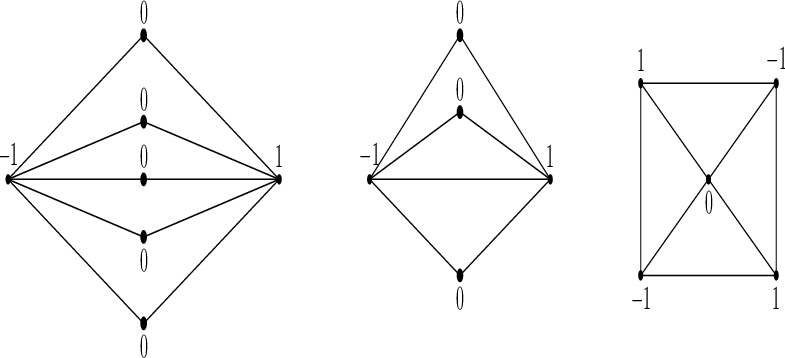
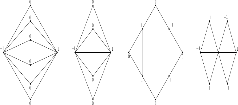
Below we give a classification by eigenvalues of the smallest trivalent graphs. Then, the transformations connecting the elements within each class generate trivalent graphs.
The smallest trivalent graph having eigenvalue (where is a non-soft vertex) satisfies . That is the path on 3 nodes shown in Fig.12.
Trivalent trees are constructed from trivalent path on 3 vertices by adding nodes between two equal-valued vertices Theorem 9 and extension of soft nodes Theorem 10. A characterization of all trees that have as the third smallest Laplacian eigenvalue is presented in [13].
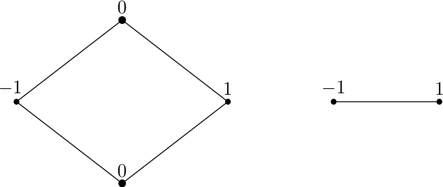
The smallest trivalent graphs having eigenvalue (where is a non-soft vertex) satisfy :
- 1.
. That is the 4-cycle shown on the left of Fig.13,
- 2.
. That is the 1-regular bivalent graph.
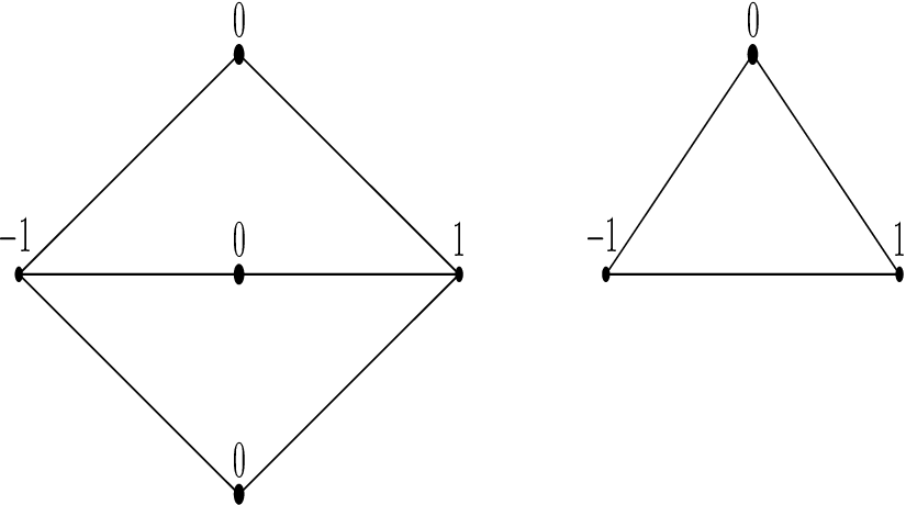
The smallest trivalent graphs having eigenvalue (where is a non-soft vertex) satisfy :
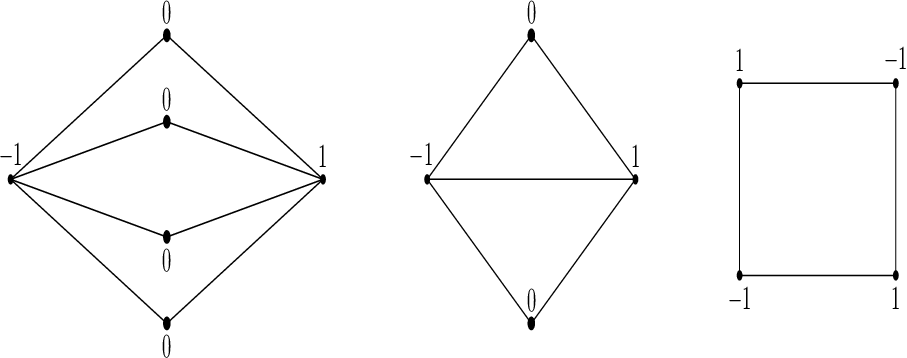
The smallest trivalent graphs having eigenvalue (where is a non-soft vertex) satisfy :
The smallest trivalent graphs having eigenvalue (where is a non-soft vertex) satisfy :
The smallest trivalent graphs having eigenvalue (where is a non-soft vertex) satisfy :
5 Conclusion
We have characterized bivalent and trivalent graphs by applying Laplacian eigenvector transformations; these are links between two equal nodes, replacing an edge by a soft square, and adding or deleting an alternate perfect matching. We show that bivalent graphs are the regular bipartite graphs and their extensions obtained by adding edges between two equal nodes. We define a soft regular graph as having a Laplacian eigenvector with soft nodes such that each non-soft node has the same degree. Trivalent graphs are shown to be the soft regular graphs and their extensions. However, the question of whether a given graph is bivalent or trivalent, is difficult and remains open. The exploration of these graphs is important for nonlinear dynamical systems on networks.
Acknowledgment
This work is part of the XTerM project, co-financed by the European Union with the European regional development fund (ERDF) and by the Normandie Regional Council.
References
- [1] J-G. Caputo, A. Knippel and E. Simo, Oscillations of networks: the role of soft nodes. Journal of Physics A: Mathematical and Theoretical 46, 035101 (2013).
- [2] D. Cvetkovic, P. Rowlinson and S. Simic, An Introduction to the Theory of Graph Spectra. London Mathematical Society Student Texts 75, Cambridge: Cambridge University Press (2010).
- [3] J-G. Caputo, I. Khames, A. Knippel and P. Panayotaros, Periodic orbits in nonlinear wave equations on networks. Journal of Physics A: Mathematical and Theoretical 50, 375101 (2017).
- [4] A. C. Scott, Nonlinear Science: Emergence and Dynamics of Coherent Structures. Oxford Texts in Applied and Engineering Mathematics 2nd edn, Oxford-New York: Oxford University Press (2003).
- [5] K. Aoki, Stable and unstable periodic orbits in the one-dimensional lattice theory. Physical Review E 94, 042209 (2016).
- [6] J-G. Caputo and A. Knippel, On graph Laplacians with eigenvectors having zero entries. Working paper (2018).
- [7]
T. Edwards, The Discrete Laplacian of a Rectangular Grid, web document (2013).
https://sites.math.washington.edu/˜reu/papers/2013/tom/Discrete %20Laplacian%20of%20a%20Rectangular%20Grid.pdf - [8] H. S. Wilf, Spectral bounds for the clique and independence numbers of graphs, Journal of Combinatorial Theory, Series B 40, 113-117 (1986).
- [9] D. Stevanović, On eigenvectors of graphs. Ars Mathematica Contemporanea Vol 11, No 2, 415-423 (2016).
- [10] R. Merris, Laplacian graph eigenvectors. Linear Algebra and its Applications 278, 221-236 (1998).
- [11] R. Merris, Laplacian matrices and graphs: a survey. Linear Algebra and its Applications 197/198, 143-176 (1994).
- [12] J. J. Molitierno and M. Neumann, On trees with perfect matchings, Linear Algebra and its Applications 362, 75-85 (2003).
- [13] S. Barik , A. K. Lal and S. Pati On trees with Laplacian eigenvalue one Journal Linear and Multilinear Algebra, Vol.56, No.6, 597-610 (2008).