Using Interaction-Based Readouts to Approach the Ultimate Limit of Detection Noise Robustness for Quantum-Enhanced Metrology in Collective Spin Systems.

The sensitivity with which we can estimate the classical parameter $\phi$ is quantified via the Cramér-Rao bound: $\Delta\phi^{2}=1/F_{C}$, where $F_{C}$ is the classical Fisher information (CFI), defined by $F_{C}=\sum_{m}\dot{P}_{m}^{2}/P_{m}$, where $P_{m}$ is the probability of obtaining measurement result $m$, and $\dot{P}_{m}\equiv\partial_{\phi}P_{m}$. Assuming a collection of $N$ particles distributed amongst two modes, the natural description for our system is provided via the pseudo-spin SU(2) algebra: $[\hat{J}_{x},\hat{J}_{y}]=i\hat{J}_{z}$ [70]. The eigenstates of these operators form a natural basis of easily accessible measurements, as they can be obtained via single-particle operations such as linear rotations and particle counting [2]. For simplicity, throughout this paper we assume that measurements are made by projecting into the $\hat{J}_{z}$ basis, i.e. , $\{\left|m\rangle\langle m\right|\}$, where $\hat{J}_{z}|m\rangle=m|m\rangle$. The particular direction is of little consequence, however, as projections along other directions can be obtained via linear rotations. Following the convention introduced in [71] and subsequently used in [69, 56, 60, 2, 50, 62, 64, 65], we model the behaviour of an imperfect detector as sampling from the probability distribution

where

introduces detection noise of magnitude $\sigma$. This is equivalent to the positive operator valued measurement (POVM) $\{\hat{M}_{m}\}=\{\sum_{m^{\prime}}\Gamma_{m,m^{\prime}}|m^{\prime}\rangle\langle m^{\prime}|\}$. To demonstrate how the noise affects the CFI, we consider the case where $P_{m}$ contains only two non-zero elements, $P_{a}$ and $P_{b}$, with $P_{b}=1-P_{a}$, and $\dot{P}_{a}=-\dot{P}_{b}=\sqrt{F_{0}(P_{a}-P_{a}^{2})}$, such that $F_{C}=F_{0}$. By approximating $m$ as a continuous variable and extending the domain to $\pm\infty$ ¹¹ 1 See the supplemental material for further details of the derivation of Eq. (7)., we obtain

Defining

(assuming $a<b$), and maximising with respect to $P_{a}$ ($P_{a}\rightarrow P_{b}\rightarrow\frac{1}{2}$) we obtain

Clearly, $F_{C}(\sigma)$ decays less rapidly when the separation between the non-zero components of $P_{m}$, $|a-b|$, is large compared to $\sigma$. This intuition leads us to postulate that distribution with maximum robustness, $P_{\mathrm{opt}}$ is

with all other elements equal to zero. While an analytic proof of this remains elusive, we confirm this via a numeric optimisation method ²² 2 See the supplemental material for further details of the optimisation method. In the absence of detection noise, the QCRB states that $F_{C}\leq F_{Q}$, where $F_{Q}$ is the QFI. We define the noisy QCRB (NQCRB) as $F_{C}(\sigma)\leq F_{n}(\sigma)$, where $F_{n}(\sigma)$ is the CFI calculated from the $\{\tilde{P}_{m}(\sigma),\dot{\tilde{P}}_{m}(\sigma)\}$ obtained from performing the discrete sum in Eq. (1) numerically with $\{P_{m},\dot{P}_{m}\}=\{P_{\mathrm{opt}},\dot{P}_{\mathrm{opt}}\}$, and setting $F_{0}=F_{Q}$. This is the maximum sensitivity that can be achieved by making spin measurements on a state with QFI equal to $F_{Q}$ in the presence of detection noise $\sigma$. We can get an approximate analytic expression for $F_{n}(\sigma)$ by again approximating $m$ as a continuous variable, but limiting the range to $-N/2<m<N/2$, such that

with $\alpha=N/\sqrt{2}\sigma$. Fig.(1) shows excellent agreement between this expression and the exact value of $F_{n}(\sigma)$, calculated numerically. Eq. (7) provides a slight under-estimate of the CFI, as information is lost when condensing $P_{m}$ into a binary distribution via Eq. (4). For the remainder of this paper, we use the exact numeric value of $F_{n}(\sigma)$ rather than Eq. (7).

The NQCRB sets the maximum achievable CFI in the presence of detection noise $\sigma$. What remains is to find an IBR that allows us to achieve this limit. Starting with an arbitrary initial pure state $|\psi_{1}\rangle$, we note that this state can always be written as $|\psi_{1}\rangle=U_{1}|\psi_{0}\rangle$, where $|\psi_{0}\rangle=|\tfrac{N}{2}\rangle$ is the maximal $\hat{J}_{z}$ eigenstate, which is completely separable in the particle basis. In most quantum enhanced metrology schemes, the unitary operator $U_{1}$ implements the state preparation step, which may be employed to increase the QFI of an initially separable state. Specific examples of this process including OAT, TACT, TNT, and QPT will be considered later. The phase shift $\phi$ is then encoded on to the state via $|\psi_{\phi}\rangle=e^{i\hat{J}_{n}\phi}|\psi_{1}\rangle$, where $\hat{J}_{n}=\mathbf{J}\cdot\mathbf{n}$, and $\mathbf{n}$ is a unit vector chosen to maximise the QFI of $|\psi_{\phi}\rangle$. This vector can be obtained from the collective covariance matrix [20]. An IBR is some unitary $U_{2}$ such that measurements are made on the state $U_{2}|\psi_{\phi}\rangle$. Our goal is to find $U_{2}$ such that the probability distribution $P_{m}=|\langle m|U_{2}|\psi_{\phi}\rangle|^{2}$ saturates the NQCRB. It was shown in [57] that for $\phi\ll 1$, selecting $U_{2}=U_{1}^{\dagger}$ saturates the QCRB. At some value $\phi=\phi_{0}$,

where

We can artificially construct an IBR that is maximally robust to noise simply by constructing a unitary operator $U_{\mathrm{p}}$ that maps this state to one with distribution $P_{\mathrm{opt}}$:

where $\{|m^{\prime}\rangle\}$ completes the orthogonal basis containing $|\frac{N}{2}\rangle$ and $|\psi^{\prime}\rangle$. Thus, the optimum IBR is

Fig. (2) shows the CFI calculated from $P_{m}=|\langle m|U_{\mathrm{opt}}|\psi_{\phi}\rangle|^{2}$ after convolving with detection noise, for quantum enhanced states generated from OAT, TACT, TNT, and QPT. Details of these states are provided in table (1) ³³ 3 For further details on these quantum states, see the supplemental material. By ‘quantum-enhanced states’, we mean ‘states with $F_{Q}>N$’. .

In all cases, we find that this IBR saturates the NQCRB. To understand the mechanism for this, we consider the effect of detection noise on the probability distributions. Fig. (3) shows $P_{m}(\phi)$ and $P_{m}(\phi+\delta\phi)$, with (right column) and without (left column) noise, for the case of OAT. When $U_{2}=U_{1}^{\dagger}$ ((a) and (e)), the change in probability is centred around $m=\frac{N}{2}$ and nearby elements. When detection noise is added, $P_{m}(\phi)$ and $P_{m}(\phi+\delta\phi)$ become less distinct as the adjacent elements are mixed. However, by applying $U_{2}=U_{\mathrm{opt}}$ ((b) and (f)), all of the probability in elements $m\neq\tfrac{N}{2}$ is transferred to $m=-\tfrac{N}{2}$ such that $P_{m}=P_{\mathrm{opt}}$. We stress that the application of $U_{\mathrm{opt}}$ does not effect the CFI in the absence of noise - the Hellinger distance

is identical in (a) and (b) ($d_{H}\approx 0.24$). However, $U_{\mathrm{opt}}$ does effect how distinguishable the states remain after the addition of detection noise: $d_{H}\approx 0.067$, and $0.201$ for (e) and (f) respectively.

While our optimum IBR gives us insight into what maximises robustness, it is of no use to us unless we can find a physical mechanism with which it can be implemented. However, we can construct an IBR which has similar properties to the ideal case with the OAT mechanism. The OAT unitary can be used to create the well known spin-cat state [75, 76]:

for even $N$ ⁴⁴ 4 For odd $N$ we require an additional rotation: an equal superposition cat is generated by $e^{i\frac{\pi}{2}\hat{J}_{y}}e^{i\frac{\pi}{2}\hat{J}_{y}^{2}}|m\rangle$.. This state has the unusual property that $|\langle\beta(m)|e^{i\tfrac{\pi}{2}\hat{J}_{z}}|\beta(m)\rangle|^{2}=\cos^{2}\frac{m\pi}{2}$. That is, even-$m$ states are unaffected by a $\pi$ rotation, while odd-$m$ states become orthogonal. As such, a $\tfrac{\pi}{2}$ phase shift followed by secondary application of $e^{i\tfrac{\pi}{2}\hat{J}_{y}^{2}}$ will return $|\beta(m)\rangle$ to $|m\rangle$ if $m$ is even, or transfer it to an orthogonal state if $m$ is odd. Specifically

The action of $U_{\mathrm{flip}}$ is to exchange the odd elements of $P_{m}$ with $P_{-m}$, while leaving the even elements unaffected, as illustrated in fig.(3) (d) and (h) ⁵⁵ 5 For odd $N$, an IBR that performs the same function is given by $U_{\mathrm{flip}}=e^{i\tfrac{\pi}{2}\hat{J}_{y}(\hat{J}_{y}+1)}e^{i\theta\hat{J}_{z}}e^{i\tfrac{\pi}{2}\hat{J}_{y}(\hat{J}_{y}+1)}$, with $\theta=\frac{\pi}{2}(1+1/N)$. For sufficiently small $\phi$, most of the CFI for the state $U_{1}^{\dagger}|\psi_{\phi}\rangle$ is usually contained in the elements $m=\tfrac{N}{2}$ and $m=\tfrac{N}{2}-1$ ((c) and (g)). Applying $U_{\mathrm{flip}}$ to this state transfers probability from $m=\tfrac{N}{2}-1$ to $m=-(\tfrac{N}{2}-1)$, forming a distribution almost as robust as $P_{\mathrm{opt}}$.

Fig. (2) shows the performance of this scheme compared to $U_{\mathrm{opt}}$ for quantum enhanced states generated via OAT, TACT, and TNT (see table (1)). In these three cases we see that $U_{2}=U_{\mathrm{flip}}U_{1}^{\dagger}$ is very close to the optimum case ($U_{2}=U_{\mathrm{opt}}$ and the NQCRB), and achieves sensitivity very close to the QCRB for detection noise $\sigma$ significantly exceeding $\sqrt{N}$. For comparison, we have also included the previously considered case of an echo, where $U_{2}=U_{1}^{\dagger}$ , which performs significantly better than the case of no IBR ($U_{2}=U_{\theta}$, where only a linear rotation is used to maximise the CFI), but not nearly as well as $U_{2}=U_{\mathrm{flip}}U_{1}^{\dagger}$. We have also included the special case of OAT with $r=\tfrac{\pi}{2}$, which corresponds to the maximum QFI spin-cat state. In this case, both $U_{2}=U_{\mathrm{flip}}U_{1}^{\dagger}$ and $U_{2}=U_{1}^{\dagger}$ saturate the NQCRB, while the case of no IBR loses all quantum enhancement for $\sigma\lessapprox 1$. The reason why there is no need for the extra application of $U_{\mathrm{flip}}$ is because the state $U_{1}^{\dagger}|\psi_{\phi}\rangle$ already yields a probability distribution identical to $P_{\mathrm{opt}}$, and is unchanged by application of $U_{\mathrm{flip}}$. The outstanding performance of the echo IBR for this state was first reported in [60] and subsequently in [61, 65], but it was not known that this is the maximum achievable sensitivity ⁶⁶ 6 We note that [61] reports higher robustness than this. However, the state is identical, and the discrepancy is due to a different convention for the detection noise.

We also considered QPT, where the increased QFI is generated by slowly varying the parameters in a time-dependent Hamiltonian, such that the ground state is adiabatically transformed to one with high QFI. We implemented this with a Hamiltonian of the form

such that

where $\mathcal{T}$ represents the time-ordering operator. In the limit $\chi t_{0}\rightarrow\infty$, $U_{1}|\tfrac{N}{2}\rangle=|0\rangle$, the twin-Fock state. We chose a moderate value $\chi t_{0}=20$, such that the final state contains non-zero elements on either side of $m=0$. Unlike the previous examples, when making measurements on the state $U_{1}^{\dagger}|\psi_{\phi}\rangle$ for small $\phi$, most of the CFI is contained in the elements $m=\tfrac{N}{2}$ and $m=\tfrac{N}{2}-2$, such that $U_{\mathrm{flip}}$ has little effect. This is easily rectified, however, by using a modified IBR with $U_{\mathrm{flip}}^{\prime}=e^{i\tfrac{\pi}{2}\hat{J}_{y}^{2}}e^{i\tfrac{\pi}{4}\hat{J}_{z}}e^{i\tfrac{\pi}{2}\hat{J}_{y}^{2}}$, which for $N\gg 1$, $U_{\mathrm{flip}}|m\rangle\approx|-m\rangle$ if $m/2$ is odd. We see in Fig. (2e) that this IBR is very close to the NQCRB.

The benefit of our IBR is not limited to pure states. We consider a quantum enhanced mixed state

We chose $\Delta=1$, which corresponds to a state with significant quantum enhancement, yet is far from pure, with the purity $\gamma=\mathrm{Tr}[\rho^{2}]\approx 0.4$. Such a state may arise from quantum enhancement via a strong QND interaction with a detuned optical field, as described in [80], with an imperfect measurement leading to uncertainty in $m$. Unlike the previous states considered, this state is mixed, so there is no unitary operator that maps this distribution to $P_{\mathrm{opt}}$. However, at $\phi=0$, the final distribution is similar to the QPT case, which inspires us to use the same IBR, namely $U_{2}=U_{\mathrm{flip}}U_{1}^{\dagger}$, with $U_{1}$ generated via the adiabatic evolution considered in the QPT example. We see in Fig. (2f) that while this case isn’t as robust as previous examples, the general trend is the same, that is $U_{2}=U_{\mathrm{flip}}U_{1}^{\dagger}$ is more robust than $U_{2}=U_{1}^{\dagger}$, which in turn outperforms $U_{2}=U_{\theta}$. As the state is mixed, we cannot systematically construct $U_{\mathrm{opt}}$. For completeness, we have also investigated applying our IBR to states with no quantum enhancement, such as coherent spin-states [81], and find qualitatively similar results ⁷⁷ 7 The plot of $F_{C}(\sigma)$ for the coherent spin state is provided in the supplementary material.

The results of this paper may form an integral part of future quantum-enhanced sensing technologies, as high-QFI states are particularly susceptible to detection noise. While OAT-based quantum enhancement schemes are not yet capable of manufacturing spin-cat states (and therefore $U_{\mathrm{flip}}$), progress in this area is rapid, particularly in schemes based on optically induced non-linearities [6, 18], and Rydberg atoms [83]. Furthermore, we have provided insight and a systematic approach for constructing a robust IBR. Armed with this insight, schemes that approximate our optimum scheme may be found through other dynamical mechanisms that are perhaps easier to implement in a particular system. For example, it has been shown that QPT can be used to engineer spin-cat states [46], so could potentially be used to construct a near-optimum IBR. One might question the wisdom of using an IBR that requires the ability to create a maximum QFI cat state in cases where the QFI of the input state is less than this. However, there may be situations when it is impractical to use a state preparation capable of creating a cat state, such as when the preparation time is limited [63]. Similarly, a state with less quantum enhancement may be desirable in the presence of external phase noise. In these situations, the presence of unavoidably large detection noise will still necessitate the use of a high-performance IBR in order to achieve high sensitivity. Finally, the NQCRB provides a limit for the performance of all IBR’s. Once the sensitivity approaches this limit, further gains can only be made through the reduction of detection noise, rather than via improvement of the IBR.

In this supplemental material I provide further details about the derivation of the noisy quantum Cramér-Rao bound (NQCRB), and provide further details about the quantum states used in this manuscript.

Beginning with Eq. (1),

and Eq. (2),

we can obtain an approximate expression for the case when $P_{m}$ contains only two non-zero elements, at $m=a$ and $m=b$. By treating the discrete probability distribution as continuous, we obtain

Replacing the discrete sum in Eq. (18) with a continuous integral, we find

where

Defining

gives

where we have used $P_{b}=1-P_{a}$. Similarly, we find

where we have used $\dot{P}_{b}=-\dot{P}_{a}$. Using these equations in $F_{C}(\sigma)=\dot{\tilde{P}}_{a}^{2}/\tilde{P}_{a}+\dot{\tilde{P}}_{b}^{2}/\tilde{P}_{b}$ gives

Setting $\dot{P}_{a}=\sqrt{F_{0}(P_{a}-P_{a}^{2})}$, such that

gives

Maximising this function with respect to $P_{a}$ (Setting $\partial_{P_{a}}F_{C}(\sigma)=0$ and solving for $P_{a}$) gives $P_{a}=\tfrac{1}{2}$, and therefore

In this section we demonstrate that of all probability distributions with $F_{C}=F_{0}$, $P_{\mathrm{opt}}$, the distribution with $P_{\tfrac{N}{2}}=P_{-\tfrac{N}{2}}=\tfrac{1}{2}$, $\dot{P}_{\tfrac{N}{2}}=-\dot{P}_{-\tfrac{N}{2}}=\sqrt{F_{0}}/2$, displays the maximum sensitivity in the presence of detection noise $\sigma$. We introduce the vectors

such that

Using this notation, its straightforward to transform our distribution such that $\mathbf{v}^{\prime}=A\mathbf{v}$, $\dot{\mathbf{v}}^{\prime}=A\dot{\mathbf{v}}$, where $A$ is a square orthogonal real matrix with the property $A^{T}A=AA^{T}=1$. Importantly, such a transformation preserves the CFI:

To confirm that $P_{\mathrm{opt}}$ is in fact the distribution with maximum robustness, we begin with an arbitrary probability distribution $P_{\mathrm{arb}}$ that satisfies $F_{C}\left[P_{\mathrm{arb}},\dot{P}_{\mathrm{arb}}\right]=F_{0}$, and then employ a numeric optimisation algorithm, which is implemented as follows:

1. 1.

   Calculate $\{\mathbf{v},\dot{\mathbf{v}}\}$ from $\{P_{m},\dot{P}_{m}\}$.

2. 2.

   Rotate $\mathbf{v}$ and $\dot{\mathbf{v}}$ by a small angle of randomly generated magnitude about a randomly generated axis in $N+1$ dimensional space. This process is represented by an orthogonal real matrix $A$, and therefore conserves $F_{C}(\sigma=0)$.

3. 3.

   Calculate $\{P_{m},\dot{P}_{m}\}$ from the new $\{\mathbf{v},\dot{\mathbf{v}}\}$.

4. 4.

   Add detection noise to this new distribution via Eq. (18) and Eq. (19), and calculate $F_{C}(\sigma)$. If the $F_{C}(\sigma)$ has increased, we accept this new distribution, and repeat. Otherwise, we keep the original distribution, and repeat.

Fig. 4 (a-c) shows the CFI after addition of detection noise for $10^{5}$ iterations of this algorithm, for three different initial distributions, all with $\dot{P}_{m}$ chosen such that $F_{C}(0)=1$. However, each distribution has a different CFI in the presence of noise. The CFI (with detection noise) rapidly converges to the CFI of $P_{\mathrm{opt}}$. The evolution of the Hellinger distance between these distributions and $P_{\mathrm{opt}}$ approaches zero (d-f). We repeated this process for several different values of $\sigma$ and initial distributions, and in all cases found convergence to $P_{\mathrm{opt}}$.

To ensure that our optimisation algorithm is not getting ‘stuck’ in a local maximum, we generate entirely random distributions satisfying the constraint that $F_{C}\left[P,\dot{P}\right]=F_{0}$, by employing a randomly generated transformation matrix to $P_{\mathrm{opt}}$. We see in Fig. (5) that while $F_{C}(0)$ remains constant, $F_{C}(\sigma)$ does not exceed the optimum value, calculated from $P_{\mathrm{opt}}$. Again, we employed different initial distributions and values of $\sigma$.

As before, we approximate $P_{\mathrm{opt}}$ as a continuous distribution such that

To derive equation (5) we made the approximation that the domain of integration extended to infinity, which is reasonable as long as $|a|,\,|b|\ll N/2$. However, in order to get a more accurate approximation, we now restrict our domain to $\{-N/2,N/2\}$. Approximating $\Gamma_{m,m^{\prime}}$ as a continuous function, and enforcing the correct normalisation conditions gives

Defining $\tilde{P}_{a}$ and $\tilde{P}_{b}$ as before, we find

and

Using these equations in $F_{C}(\sigma)=\dot{\tilde{P}}^{2}_{a}/P_{a}+\dot{\tilde{P}}^{2}_{b}/P_{b}$ gives

If we choose our IBRO such that the measurement saturates the QCRB in the absence of noise, we replace $F_{0}$ with $F_{Q}$, and arrive at equation (6) of the main text.

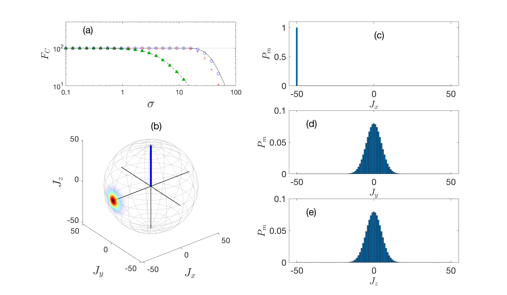
In this section we give further details about the states used in figure (2) of the main text. We have used the Husimi $Q$-function as a visualisation tool, defined by

with $\rho=\left|\psi_{1}\rangle\langle\psi_{1}\right|$, and

Additionally, $N=100$ was used throughout.