Scrambling and entanglement spreading in long-range spin chains
Abstract
We study scrambling in connection to multipartite entanglement dynamics in regular and chaotic long-range spin chains, characterized by a well defined semi-classical limit. For regular dynamics, scrambling and entanglement dynamics are found to be very different: up to the Ehrenfest time, they rise side by side departing only afterward. Entanglement saturates and becomes extensively multipartite, while scrambling, characterized by the dynamic of the square commutator of initially commuting variables, continues its growth up to the recurrence time. Remarkably, the exponential growth of the latter emerges not only in the chaotic case but also in the regular one, when the dynamics occurs at a dynamical critical point.
I Introduction
Classical systems with long-range interactioruns display many interesting dynamical properties that have been extensively studied since many
decades [1]. In the quantum domain, instead, long-range systems have been the focus of a great deal of attention
only lately, as a result of their experimental simulation with different platforms [2, 3, 5, 4]. These systems allow the controlled study of quantum dynamics in the absence of significant decoherence, a property that
allows the study of a number of important phenomena as, for example, dynamical phase transitions [6, 8, 7]
or the dynamics of correlations [9, 10, 11, 12, 13] in a situation where Lieb-Robinson bounds do not apply [14, 15].
It is well established that understanding the coherent dynamics of a quantum many-body system requires a thorough understanding of the behaviour of its quantum correlations [16, 17]. The spreading of quantum correlations has been the focus of a lot of
theoretical efforts [18], starting from the initial important results on the dynamics of entanglement entropy [19].
Very recently a new way to characterise quantum dynamics of many-body systems has been proposed, based on the concept of scrambling. Initially introduced
as a probe of quantum chaos [20, 21, 22, 21, 23], scrambling is generically identified as the delocalisation of quantum information [24] in a many-body system. A measure of scrambling is associated with the growth of the square commutator between two initially commuting observables [20, 21]. For quantum chaotic systems [20, 21, 25, 26], this quantity is expected to grow exponentially before the Ehrenfest time - defined as the time at which semi-classics breaks and quantum effect become dominant [56]- otherwise, it grows at most polynomially in time [28, 27, 29].
Despite the impressive progress over the last years, several different questions related to scrambling and entanglement propagation still await a more detailed answer. It has been observed that the exponential growth of the square commutator is connected to the chaotic behaviour of an underlying semi-classical limit. The precise role of semiclassical correlations in determining scrambling dynamics and its various stages are presently under intense study [30, 31, 32]. Furthermore, in view of the various forms in which quantum correlations manifests in a many-body system, it is important to understand how entanglement is connected to the scrambling of information. A first connection between square commutators and the spreading of quantum entanglement has been made in the context of unitary quantum channels [33, 34]. An analysis of different velocities of propagation of information has been performed in [24], while connections of scrambling to the growth of Rényi entropies and multiple-quantum coherence spectra have been investigated in [35, 36, 37]. In long-range systems, scrambling has been studied in connection to correlation bounds [13, 38] and its time average as a probe of criticality [39].
However, an analysis of the dynamics and the relevant time-scales in relation to the different processes involved in the spreading of information is still missing.
In this work, we address all these questions by studying multipartite entanglement propagation and scrambling in spin chains with long-range interaction either subject to a quantum quench or a periodic drive.
There are several reasons behind this choice. Spin chains with long-range interactions possess a well defined semiclassical limit, and thus represent a natural playground [40] to study the role of classical correlations in scrambling. Furthermore, they allow exploring the transition from semiclassical to quantum dominated regimes in the dynamical behaviour. We will consider both the case of integrable and chaotic dynamics. Moreover,
scrambling is experimentally accessible with long-range quantum simulators, as it has been measured for unitary operators [41].
We will present results for the entanglement dynamics of the quantum Fisher information, the tripartite mutual information and operator scrambling, studied via the square commutator. As we are going to show in the rest of the paper scrambling and entanglement dynamics turn out to be very different.
| Quantum quench | Quench at DPT | Periodic kicking | ||
|---|---|---|---|---|
| Scrambling | ||||
| const. | ||||
| Entanglement | growth | peak | growth | |
| const. | const. | const. |
The paper is organized as follows. The next section is devoted to a summary of the results with a direct comparison between multipartite entanglement growth and scrambling. In section III, we review the long-range version of the Ising chain and the type of dynamics that are considered across the paper. We recall the semiclassical limit together with the quantum and classical characterization of chaos. In section IV, we briefly review the definitions of the quantities under consideration: the quantum Fisher information, the tripartite mutual information, and the square commutator. In section V we describe the different numerical and the semi-analytical methods used to reproduce the behavior of the square-commutator. We first present in section VI.1 the results for the entanglement dynamics and its semiclassical nature for sufficiently long-range interaction. We discuss how this behavior changes when the range of the interaction is decreased. Then, in section VI.2, we consider the results for the square-commutator and we argue that the long-time dynamics of the square commutator accounts for the quantum chaoticity of the dynamics. We provide evidence for our claims by discussing an example of an exponential growth of scrambling in the case of a regular quantum dynamics. Section VII is devoted to our conclusions.
II Main results
In this paper, we study how entanglement and operator’s scrambling grow and spread in Ising spin chains with two-body power-law decaying interactions, . We consider the case in which an initial separable state, i.e. , is brought out-of-equilibrium by means of a quantum quench or a periodic drive. Our findings can be summarized as follows:
- 1.
Entanglement dynamics reflects the semi-classical nature of the system: it is weak, slowly growing and saturating at the Ehrenfest time . This is what lies at the heart of the classical “simulability” of quantum long-range interacting systems in the context of MPS-TDVP [43, 42] with small bond-dimension as well as semiclassical methods [44, 45, 46].
- 2.
The square commutator is characterized by two different regimes, a first semiclassical growth up to the (exponential for chaotic dynamics), followed by a fully quantum non-perturbative polynomial growth (saturation for chaotic dynamics), symmetric around the recurrence time . We show that the initial growth encodes the nature of classical orbits and can be exponential also for regular integrable dynamics, provided they have some classical instabilities. Conversely, the second regime accounts for the quantum chaoticity of the dynamics, see table 1.
- 3.
The dynamics of the information spreading changes with the range of interaction . The Hamiltonian with is dominated by the classical limit and the structure of entanglement and scrambling is the same as in the infinite range case, see table 1. For , the entanglement grows linearly in time and the structure of the asymptotic state is the same as for . For the state displays the typical entanglement dynamics and structure of short-range interacting systems, with negative TMI.
This shows that state’s entanglement growth and operator’s scrambling are two distinct, apparently disconnected phenomena. Interestingly, this becomes glaringly obvious in the regular regime, rather than in the chaotic one, see Fig.4.
III The model and out-of-equilibrium protocols
We consider an Ising chain in transverse field with long-range interactions,
| (1) |
where are spin operators and and is
the Kac normalization [47]. The (solvable) infinite range limit of Eq.(1) is known as the Lipkin-Meshov-Glick model
(LMG) [48] and it has been intensively studied out-of-equilibrium [49, 6, 50, 51, 52]. In this case the Hamiltonian conserves the total spin and we restrict our analysis to the sector of the ground-state . This has a
semiclassical limit before , controlled by , where the system can be described classically in terms of only two degrees of freedom and
a classical Hamiltonian [49, 6, 50]. For finite , ground states of the Hamiltonian of Eq.(1) can be
seen as coherent wave-packets with width that evolve for short times classically [6]. The semi-classical dynamics is discussed in details in next section. As far as the dynamics of local observables is concerned, the Hamiltonian of Eq.(1) is
found to behave as the infinite range for , as a short-range one for [7, 10].
Taking an initial separable state totally polarised along the axis
, we probe entanglement dynamics and scrambling with the two following protocols.
Quantum quench
The state is evolved with the Hamiltonian (1) with a transverse field . For , a special case, important also for the present analysis, is represented by where a dynamical phase transition (DPT) occurs [53], whose origin can be traced back to the corresponding classical dynamics. Away from the dynamical critical point the Ehrenfest time reads while at the
dynamical critical point . It was shown in [39] that DPT can be detected with the
average value of out-of-time correlators.
Periodic kicking
In order to address chaotic dynamics in long-range spin system we will also consider the case in which periodic kicks are added to the evolution governed by Eq.(1), with . This model, known also as the “kicked top” for , is a paradigmatic example of the standard quantum chaos [54, 55]. The time-evolution operator over one period reads
| (2) |
III.1 Semiclassical phase-space
Let us recall the main features of the semiclassical dynamics. Since the Hamiltonian of Eq.(1) commutes with the total spin , we restrict ourself to the spin sub-sector of the ground state , where the dimensionality of the Hilbert space is . Defining , we can re-express the LMG Hamiltonian in terms of its components
| (3) |
This allows to consider an effective that identifies the semiclassical limit with the large- mean field one. In what follows we set . In this limit, the system is effectively described by the classical Hamiltonian
| (4) |
where the two conjugate variables are given in terms of the expectation values of on a wave packet as , and and obey to the classical Hamilton equations, [49, 6, 50].
In the sudden quench case, the ground state at is evolved with the hamiltonian with transverse field . The dynamical phase transition DPT between a finite and zero order parameter occurs at . One can define a dynamical order parameter as the average magnetization in time: , which is different from zero in the symmetry broken phase. Indeed, at the phase point associated to the initial ground state energy (which is conserved) lays right on the separatrix of the final Hamiltonian: for it orbits around the maximum with a , while for it orbits around one of the two ferromagnetic minima and , see Fig.1.
When the kicking is added, the total classical Hamiltonian reads
| (5) |
where : the classical kicking acts every period like a rotation around the axis with an angle proportional to . In the numerical calculations, we re-express the Hamilton’s equation of motion as equation of motions for the spin-components
| (6) |

Note that these equations can be obtained also from the expectation value of the Heisenberg equation of motion, setting to zero the second order cumulant. This is justified by the fact that the magnetization components commute in the classical limit: . In the limit of large but finite , one can consider the semiclassical WKB approximation [6] and explore wave-packet dynamics. In this framework, ground states of can be seen as coherent wave packets with width . This semiclassical picture holds until the states behave like well defined wave-packets. It is then natural to define the time for which semi-classics breaks down- the Ehrenfest time - as the time for which the initially coherent wave-packet is spread and delocalized. It is well known that this depends on the nature of the classical dynamics [56]
| (7) |
where is the Largest Lyapunov exponent of the classical dynamics in the chaotic case.
III.2 Characterization of chaos
In the quantum realm, an important signature of chaos is provided by the spectral properties of the evolution operator, in our case by the properties of the Floquet spectrum. The distribution of the Floquet level spacings (the are in increasing order), normalized by the average density of states, gives information on the integrability and ergodicity properties of the system [55, 57, 58, 59]: if the distribution is Poisson, then the system is integrable; if it is Wigner-Dyson, then the system is ergodic.
In order to probe the integrability/ergodicity properties through the level spacing distribution, we consider the so-called level spacing ratio
| (8) |
The different level spacing distributions are characterized by a different value of the average over the distribution. From the results of Ref. [60], we expect if the system behaves integrably and the distribution is Poisson; on the other side, if the distribution is Wigner-Dyson and the system behaves ergodically, then . In our case, the Floquet levels fall in two symmetry classes, according with the corresponding Floquet state being an eigenstate of eigenvalue or of the operator under which the Hamiltonian is symmetric [54]. Therfore we need to evaluate the level spacing distribution and the corresponding only over Floquet states in one of the symmetry sectors of the Hamiltonian. The level spacing ratio for this model is reported in Fig.2 as a function of the kicking strength : it shows a transition from a regular to a chaotic regime.
The relationship between classical chaos and the properties of the many-body quantum dynamics has been widely studied in the past, giving rise to a plethora of signatures of chaos in the quantum domain [55, 57]. Classically, a system is ergodic if all the trajectories uniformly explore the accessible part of the phase space. In case of few degrees of freedom, a qualitative measure of this phenomenon is the Poincaré section:
some initial values are evolved under the stroboscopic
dynamics reporting on a plot the sequence of their
positions. If the initial condition lies in a regular region of
the phase space, our points will be over a one-dimensional
manifold. If instead, the initial condition is in a chaotic region of
the phase space, our points will fill a two-dimensional portion
of phase space. The model under analysis satisfies this conditions in the semi-classical limit, see Fig.1.
IV Characterization of entanglement and scrambling
Let us now introduce the quantities that we will use to characterize entanglement and scrambling.
As far as the entanglement is concerned, we will focus on the multipartite case (bipartite entanglement was already studied in [61, 62]). The characterisation of multipartite entanglement is more delicate than that of bipartite entanglement since there exist a zoo of possible measures and witnesses. We will focus here on the quantum Fisher information (QFI) and on the tripartite mutual information (TMI) [33], which accounts for the information delocalization. Scrambling is instead studied via the square commutator .
The quantum Fisher information is a witness of multipartite entanglement which has been shown
to obey scaling at the equilibrium transition point [63] and is connected to the diagonal ensemble in the
non-equilibrium case [64].
The QFI gives a bound on the size of the biggest entangled block. For example, given a system
of spins, if the QFI density , then there are at least entangled spins [65, 66].
For pure states, the QFI is given by an optimization over a generic linear combination of local spin operators of .
Here, we consider collective spin operators and we maximise over the three directions.
The tripartite mutual information is defined as where are four partitions and the quantity is the mutual information between . This takes into account information about A that is non-locally stored in and such that local measurements of and alone are not able to re-construct . Usually is associated with the delocalisation of quantum information in the context of unitary quantum channels [33]. In this case, more appropriately, we study the delocalisation of the initial state information under the dynamics, which is a complementary measure of entanglement.
Finally, in order to characterise the dynamics of scrambling, we will focus on the square commutator . This object measures the non-commutativity induced by the dynamics between two initially commuting operators and . It was introduced by Larkin and Ovchinnikov in [20], to describe semiclassically the exponential sensitivity to initial conditions and the associated Lyapunov exponent. By taking collective spin operators [29] , the square commutator has a natural classical limit for [67]
| (9) |
where on a coherent wave packet, are the Poisson brackets of the corresponding classical trajectory and the average is performed over an initial phase-space distribution.
V Methods
The results presented in this work were obtained with a series of numerical techniques and two semi-analytical approximations.
The numerical methods are a combination of exact diagonalization (ED) and well-established semi-classical approximations which are based on Wigner phase-space representations: the truncated Wigner approximation (TWA) [68] on the continuum phase-space and the discrete truncated Wigner approximation (DTWA) [69, 45] of the finite dimensional phase space. To this end, we generalised the corresponding expression for the square commutator to the discrete phase space representation, see Eq.(20) and the supplementary material for the details used in our calculations. All these approaches neglect terms of the order of and give the same results up to the Ehrenfest time. DTWA, in particular, is able to reproduce also entanglement long-time dynamics.
Furthermore, we also adopted the matrix product state time-dependent variational principle (MPS-TDVP) [42, 43], for the dynamics of long-range hamiltonians with .
We combine these approaches with two semi-analytical methods in order to predict the behavior of up to .
The first method is a equation of motion closure at fifth order: it consists in deriving a hierarchy of differential equations for the square commutator and in closing it by setting the fifth order cumulant to zero. This allows to decouple the higher order commutator and to close the system of equations. By setting the appropriate initial conditions, one can integrate numerically the equations and get the approximated . The second method is a time-dependent Holstein Primakoff and it consists in including quantum fluctuations on top of the classical result and to keep it only at the Gaussian level. These approaches turn out to be equivalent and to correctly reproduce before as in Fig.3. The following two paragraphs are devoted to a description of these approximations.
Equation of motion closure at fifth order
The cumulant closure at order is a general method that consists in closing a set of differential equations, by setting to zero all cumulants of the order . A very easy example is the cumulant closure at second order, which allows computing the classical equation of motion for the magnetization of Eq.(6).
We are interested in the dynamics of the square commutator and we wish to find a set of differential equations that gives its evolution.
One first defines a symmetric -string commutator
| (10) |
where there are time-dependent operators and two time-independent ones. Within this notation, the square commutator of Eq.(1) reads . The dynamics will generate an infinite number of coupled equations of motion. We close this hierarchy of differential equations by setting the fifth order cumulant to zero: . If one assumes that the magnetization is classical (second order cumulant set to zero), the -string commutator decouples in
| (11) |
for . This allows to close the hierarchy of differential equations, which are coupled to the classical magnetization dynamics of Eq.(6) as
| (12) |
These equations are integrated numerically via a fourth order Runge-Kutta method. The information about the initial state and the dimension of the system is encoded in the initial conditions. The that we obtain with this cumulant closure turns out to reproduce the limit of all these semiclassical approximations. It well reproduces the exact , up to a time (see Fig.3).
Time-dependent Holstein Primakoff
In a spin wave expansion, quantum fluctuations are treated as small fluctuations on top of the classical solution [70].
One first produces a time-dependent rotation of the reference frame , in such a way that the axis follows the motion of the classical collective spin . Then an Holstein-Primakoff transformation is performed and the quantum fluctuations are kept at the gaussian order. In this rotating frame the collective spin operators are the zero-mode components in the Fourier transform: , with . Our approximation consists in taking the operator on the -axis not varying in time: . This allows to compute commutators in the rotating frame, hence to get an approximated solution for .
The main steps to solve the dynamics are the following [70]:
- •
perform a time dependent unitary rotation with ; the angles are chosen such that . In the new frame the operators evolve with ;
- •
perform an Holstein-Primakoff transformation on the operators in in terms of the conjugate variables ;
- •
keep only Gaussian terms, which is equivalent to neglect all terms in the equations.
With such a choice one remains with the following hamiltonian
| (13) |
Then, by setting , one gets the equation of motion for the rotating frame, see [71]
| (14) |
In the same way one can obtain the Heisenberg equation of motion for for . Further defining the zero-mode fluctuations as
| (15a) | ||||
| (15b) | ||||
| (15c) | ||||
and combining them with the equations for , one gets the equations of motion for the zero-mode fluctuations
| (16) |
They are a set of linear time-dependent differential equations, which can be solved numerically with the appropriate initial conditions. They are exactly the quantities that appear in the computation of the square commutator. In order to compute it perform first a rotation to with , then compute commutators like , noticing that , hence at this order they are equal-time commutators that give rise to the zero mode fluctuations of Eq.(15). For example our square commutator of Eq.(3) reads as
| (17) |
which can be obtained numerically from the integration of Eq.(16) and gives exactly the same result of the previous approximation, see Fig.3. This is correct until the spin-wave density remains small, which, for finite , occurs before .
Notice that this method could be in principle extended to long range systems with and other variations of fully connected models [70]. In addition one could in principle go beyond the gaussian approximation by keeping the interaction between spin waves.
VI Results
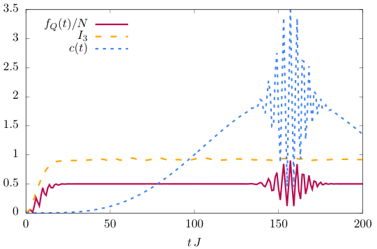
As we hinted out at the beginning of the paper, entanglement and scrambling are two different phenomena, characterized by different time scales, see Fig.4. Let us now finally describe in details the results obtained for the dynamics of entanglement and scrambling using the methods described before.
VI.1 Entanglement dynamics
In the infinite range model, entanglement dynamics and information delocalisation reflect the semiclassical nature of the system under analysis. We start discussing the dynamics governed by Eq.(1) after a quantum quench and describe afterward the case of the periodic kicking protocol.
Let us focus first on the LMG model at . Both and have the same dynamics; growth followed by saturation at , as dictated by the semiclassical dynamics of the model, see Fig.5 (top and middle panels). The stationary state displays global entanglement of genuine multipartite nature , where is a function of the transverse field. The value of the phase along the direction can be computed analytically in terms of elliptic integrals. Following Ref. [71], with a combination of the classical equation of motion and energy conservation, defining , one gets
| (18) |
where are the elliptic integrals of first and second kind of amplitude , modulus and is the inversion point of the classical trajectory . The maximum asymptotic entanglement witnessed by the QFI is , which occurs when the system from a product state is quenched to the maximally paramagnetic phase and corresponds to the biggest fluctuations of the collective spin operators.
The TMI gives complementary information: being positive, it shows that the information of the initial state is not
delocalised across the system. Interestingly, by increasing the TMI becomes negative
, see Fig.6.

Let us spend a few words for the quench to the DPT, which occurs at , see Sec.III. In this case, the entanglement dynamics is qualitatively different. QFI and TMI at short times peak at . After a transient they reach their stationary value, which keeps oscillating without recurrences, see Fig.5. This behavior is tightly linked to the existence itself of the DPT, that corresponds to a classical separatrix in phase space: the effective classical trajectory takes time of the order of to depart from its initial value. After that, the classical picture is lost and the state is spread over the basis giving a constant entanglement, see Fig.S3.
The entanglement dynamics is reproduced, up to very long times, by a semiclassical approach. We studied this regime using DTWA, spin-wave theory and cumulant closure methods, see Sec.V. All these approaches neglect terms of the order of and give the same results up to the Ehrenfest time.
The accuracy of all the semiclassical analysis is justified by the entanglement structure itself. In fact, this is what lies at the heart of the classical “simulability” of quantum long-range interacting systems in the context of MPS-TDVP [43, 42] and with semiclassical methods [44, 45, 46]. DTWA, in particular, is able to reproduce
also the long-time dynamics even beyond the recurrence time as shown in Fig.5 (bottom panel). This is due to the fact that method averages over an extensive number of trajectories, hence mimicking a discreteness of the spectrum, responsible for the recurrences [45].
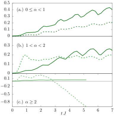
The same asymptotic structure and dynamics is found for all mean-field like systems
: the QFI grows linearly in time up to a value , and the TMI increases logarithmically in time up to a constant value. For , the QFI and the TMI grow linearly in time and the entanglement structure of the asymptotic state is the same as for . Decreasing the range of interaction the situation changes drastically: for the state displays the typical dynamics and structure of short-range interacting systems
; interestingly signaling that the information about the initial condition is spread throughout the degrees
of freedom of the state (see Fig.6). The results are obtained with TDVP, see the supplementary material for a discussion of the convergence of the method.

Finally, we conclude the analysis of the multipartite entanglement by considering the kicked case in the regime when the dynamics is chaotic. This system heats up to a state where all local observables on any Floquet state correspond to the infinite temperature values [54]. All quantities characterizing entanglement quantities saturate to an asymptotic value at the Ehrenfest time , for every initial state and field , see Fig.S4 of the supplementary. The value of the QFI, being a sum of local observables, is compatible with the values of the infinite temperature state: . On the other side, the entanglement entropy saturates to the value expected for a random state, which was derived by Page in [72] with the dimensions of the Hilbert space of the two subsystems and . In this case, for a partition of size the dimensions are , and . This reflects on the TMI and we find
| (19) | ||||

VI.2 Scrambling
Scrambling, as measured by the square commutator, behaves in a profoundly different way from entanglement. It is characterised by an initial semi-classical regime and a second quantum non-perturbative growth. Interestingly, this phenomenon is very evident in the regular regime (Fig.7), and it is much less clear in the chaotic one (Fig.8) already discussed at the beginning of the paper.
In the case of the quench dynamics, for the square commutator is characterised by a first semiclassical quadratic growth until . In this regime, semiclassical approximations describe very well the evolution of and we chose to employ DTWA. To this end, we generalised the corresponding expression for the square commutator to the discrete phase space representation
| (20) |
where , with the Weyl transform of the spin operators and the average is computed over the initial discrete Wigner distribution, see the supplementary material. At the quantum regime starts, characterised by a polynomial growth up to a maximum . At this time, the square commutator is independent of the system size. Even the DTWA, that perfectly reproduces multipartite entanglement dynamics up to (see Fig.5) is not able to reproduce the long time dynamics of the square commutator, see Fig.7. Indeed DTWA, despite keeping discrete trajectories, represents all operators as factorised on each site at any time [45]. At times longer than , the operator expansion starts developing longer and longer strings and the square commutator re-sums all the correlations, until , which corresponds to the time at which the string of length occurs. Quenches to are characterized by the same time-scales and and the same semi-classical regime up to . The result at long-times is qualitatively different: the quantum regime is and goes to zero at all times in the thermodynamic limit. This is a direct consequence of the existence of the dynamical transition, which is detected by scrambling [39]. Due to the presence of a macroscopic magnetization, the support of the operators has a constrained dynamics and it will not acquire a string of length .
A special case is represented by the quench at ; despite the integrability of the quantum system, we find that the square commutator grows exponentially in time up to as . This is due to the existence of the unstable trajectory in the classical dynamics. The exponent is twice the eigenvalue of the instability matrix of the separatrix trajectory for . This is valid in general for all the classical trajectories associated with DPT. To our knowledge, it is the only example of an early time exponential growth in a many-body regular system. After , keeps growing linearly in time up to the and then it goes back, see Fig.8. Long-range interactions do not change drastically this finding. In the range , the early time dynamics is the same as that described before. The square commutator grows like a power law at small times, even for .
We conclude by considering the kicking, which induces a chaotic dynamics. As expected, is initially dominated by the classical exponential
growth, then, as , quantum interference effects appear and the square commutator saturates to a constant value [67],
see Fig.8 (lower panels). In the quantum chaotic regime, the dynamics are reproduced by the semiclassical approximation,
which predicts the initial time growth of the square-commutator. After , the TWA loses any physical meaning. The quantum remains constant and finite in the thermodynamic limit, meaning that the operator’s support is spread up to the longest string already from
. Notice that in this case, the exponent is different from the actual classical Lyapunov exponent, defined as
, that we compute following [73].
As pointed out by [30], this difference comes from a different ordering in evaluating the phase-space averages.
VII Conclusions
In this work, we performed an analysis of the spreading of multipartite entanglement in long-range spin systems in comparison to that of scrambling. We show that quantum correlations build up and spread in different ways. While entanglement and the delocalization of the state’s information are state properties, scrambling instead describes the growth of quantum correlations in operator’s space.
After a quantum quench in the transverse field of the infinite range hamiltonian, entanglement is seen to saturate and become extensively multipartite at . On the same timescale, the TMI saturates to a positive value , showing that the information of the initial state is not delocalized across the system. In this case, entanglement dynamics is reproduced, up to very long times, by all the semiclassical approaches.
On the other end, scrambling, as characterized by the square commutator of collective spin operators, increases semiclassically up to , continuing its growth even afterward up to the recurrence time. Particularly interesting is that, despite the dynamics being regular, the early-time exponential behaviour emerges when the dynamics occur at the critical point of the dynamical phase transition, see Fig.8. This point is associated with an unstable trajectory on the effective classical phase-space [6] and the exponent of the square commutator is twice the eigenvalue of the instability matrix of the separatrix trajectory. Nonetheless, being the quantum dynamics regular, after , the square commutator keeps growing linearly in time up to the regular , see Fig.8. The other quenches, as in Fig.4, are characterized by a first growth up to which is followed by a polynomial quantum
regime up to .
In the presence of a periodic kicking for the chaotic evolution, entanglement saturates at to values compatible with the infinite temperature state. As far as scrambling is concerned, we recover the exponential growth of the square commutators expected for chaotic systems up to , followed by the corresponding saturation induced by quantum interference effects, see Fig.8.
We conclude the summary of our results, by considering the case in which a quantum quench is performed with . In this case, we employ TDVP and semi-classical analysis. Entanglement has the same asymptotic structure and dynamics within the interaction range : the QFI grows linearly in time up to a value , and the TMI increases logarithmically in time up to a constant value. For , the QFI and the TMI grow linearly in time and the entanglement structure of the asymptotic state is the same as for . Decreasing the range of interaction the situation changes: for the state displays the typical dynamics and structure of short-range interacting systems
; interestingly signaling that the information about the initial condition is spread throughout the degrees of freedom of the state (see Fig.6). Coming to scrambling, we find that before for , the square commutator grows as .
Despite entanglement can be efficiently reproduced up to very long times by our numerical tools, they all fail in predicting scrambling after . In our understanding, this follows from the fact that all methods approximate the support of the operator to remain factorized on the initial basis. Such approximations do not allow to reproduce the non-local behavior of scrambling at long-times. We would like to stress that the quantum regime of scrambling, which arises after is not peculiar only of our models or of regular dynamics. In fact, a power law in the quantum regime has been found also in chaotic systems [75, 74]. The long-time behavior of the square commutator shows the presence of purely quantum correlations that build up in the operator space. In this respect, it would be interesting to explore new quantum information protocols that encode information in the operator itself.
Acknowledgements.
We acknowledge useful discussions with J. Goold, A. Lerose and A. Polkovnikov. We acknowledge support from EU through project QUIC under grant agreement 641122, the National Research Foundation of Singapore (CRP - QSYNC). B. Z. is supported by the Advanced grant of the European Research Council (ERC), No. 694544 – OMNES.References
- [1] A. Campa, T. Dauxois, D. Fanelli and S. Ruffo, Physics of long-range interacting systems, Oxford University Press (Oxford, 2014).
- [2] M. Albiez, R. Gati, J. Fölling, S. Hunsmann, M. Cristiani, and M. K. Oberthaler, Phys. Rev. Lett. 95, 010402 (2005).
- [3] R. Blatt and C. Roos, Nat. Phys. 8, 277 (2012).
- [4] P. Jurcevic, H. Shen, P. Hauke, C. Maier, T. Brydges, C. Hempel, B. P. Lanyon, M. Heyl, R. Blatt, and C. F. Roos, Phys. Rev. Lett. 119, 080501 (2017).
- [5] B. Neyenhuis, J.. Smith, A. C. Lee, J. Zhang, P. Richerme, P. W. Hess, Z. - X. Gong, A. V. Gorshkov, and C. Monroe, Science Adv. 3, e1700672 (2017).
- [6] B. Sciolla and G. Biroli, Journ. of Stat. Mech: Th. and Exp. 11, P11003 (2011).
- [7] B. Žunkovič, M. Heyl, M. Knap and A. Silva, Phys. Rev. Lett., 120, 130601., (2018).
- [8] E.A. Yuzbashyan, O. Tsyplyatyev and B.L. Altshuler, Phys. Rev. Lett., 96, 097005, (2006).
- [9] P. Hauke and L. Tagliacozzo. Phys. Rev. Lett. 111, 207202 (2013)
- [10] L. Cevolani, G. Carleo and L. Sanchez-Palencia, New J.Phys., 18, 093002, (2016).
- [11] Z.X. Gong, M. Foss-Feig, S. Michalakis and A.V. Gorshkov, Phys. Rev. Lett.,113, 030602, (2014).
- [12] M. Foss-Feig, Z.X. Gong, C.W. Clark and A.V. Gorshkov, Phys. Rev. Lett., 114, 157201, (2015).
- [13] D.J. Luitz and Y. Bar Lev, arXiv preprint arXiv:1805.06895, (2018).
- [14] E. Lieb, D. Robinson, Commun. Math. Phys. 28, 251 (1972).
- [15] M. B. Hastings and T. Koma, Commun. Math. Phys. 265, 3, (2006).
- [16] L. Amico, R. Fazio, A. Osterloh, and V. Vedral, Rev. Mod. Phys. 80, 517 (2008).
- [17] J. Eisert, M. Cramer, and M. B. Plenio. Rev. Mod. Phys. 82, 277 (2010).
- [18] P. Calabrese, J. Cardy, and B. Doyon Eds, J. Phys. A 42, 500301 (2009).
- [19] P. Calabrese and J. Cardy, J. Stat. Mech. 2005, 04, (2005).
- [20] A.I. Larkin and Y.N. Ovchinnikov, Sov Phys JETP 28, 1200-1205, (1969).
- [21] A. Kitaev, Talks at KITP, April 7, 2015 and May 27, (2015).
- [22] J. Maldacena and D. Stanford, Phys. Rev. D 94, 106002, (2016).
- [23] J. Maldacena, S. H. Shenker, and D. Stanford, JHEP, 106, (2016).
- [24] M.Mezei and D.Stanford. JHEP, 2017, 65, (2017).
- [25] I.L. Aleiner, L. Faoro and L.B. Ioffe, Ann. Phys. , 375, 378, (2016).
- [26] A.A. Patel and S. Sachdev, Proc. Nat. Acad. Sciences, 114, 1844, (2017).
- [27] B. Swingle and D. Chowdhury, Phys. Rev. B, 95, 060201, (2017).
- [28] X. Chen, T. Zhou, D.A. Huse, E. Fradkin, Ann. Physik, 529, 1600332 (2017).
- [29] I. Kukuljan, S. Grozdanov and T. Prosen, Phys. Rev. B, 96, 060301, (2017).
- [30] E.B. Rozenbaum, S. Ganeshan, and V. Galitski, Phys. Rev. Lett., 118, 086801, (2017).
- [31] T. Scaffidi and E. Altman, arXiv:1711.04768 (2017).
- [32] J. Rammensee, J.D. Urbina and K. Richter, arXiv preprint arXiv:1805.06377, (2018).
- [33] P. Hosur, X.L. Qi, D.A. Roberts and B. Yoshida, JHEP 2, 4, (2016).
- [34] D. Ding, P. Hayden and M. Walter,J HEP, 12, 145, (2016).
- [35] C. von Keyserlingk, T. Rakovszky, F. Pollmann and S. Sondhi, S. arXiv preprint arXiv:1705.08910, (2017).
- [36] Z.W. Liu, S. Lloyd, E.Y. Zhu, and H. Zhu, Phys. Revi. Lett., 120, 130502, (2018).
- [37] M. Gärttner, P. Hauke and A.M. Rey, Phys. Rev. Lett. 120, 040402, 2018). Chen, X.,
- [38] X. Chen, T. Zhou and C. Xu, arXiv preprint arXiv:1712.06054, (2017).
- [39] M. Heyl, F. Pollmann, B. Dóra, arXiv preprint arXiv:1801.01684, (2018).
- [40] B. Swingle, G. Bentsen, M. Schleier-Smith and P. Hayden, Phys. Rev. A, 94, 040302, (2016).
- [41] M. Gärttner, J.G. Bohnet, A. Safavi-Naini, M.L. Wall, J.J. Bollinger and A.M. Rey, Nature Physics, 13, 781, (2017).
- [42] J. Haegeman, C. Lubich,I. Oseledets, B. Vandereycken, and F. Verstraete, Phys. Rev. B, 94, 165116, (2016).
- [43] J. Haegeman, J. I. Cirac, T. J. Osborne, I. Pižorn, I. Verschelde and F. Verstraete, Phys. Rev. Lett., 107, 070601, (2011).
- [44] A. Polkovnikov, Annals of Physics 325, 1790-1852, (2010).
- [45] J. Schachenmayer, A. Pikovski, and A. M. Rey, Phys. Rev. X, 5, 011022 (2015).
- [46] J. Wurtz, A. Polkovnikov, D. Sels - arXiv preprint arXiv:1804.10217, (2018).
- [47] M. Kac, J. Math. Phys., 4, 216, (1963).
- [48] H.J. Lipkin, N. Meshkov and A. J. Glick, Nuclear Physics 62 (1965): 188-198.
- [49] V. Bapst and G. Semerjian, Journ. of Stat. Mech: Th. and Exp. 2012, P06007, (2012).
- [50] A. Russomanno, R. Fazio and G. E. Santoro, EPL 110, 37005, (2015).
- [51] I. Homrighausen, N.O. Abeling, V. Zauner-Stauber and J.C. Halimeh, Phys. Rev. B, 96, 104436, (2017).
- [52] J. Lang, B. Frank, J.C. Halimeh, Phys. Rev. B, 97, 174401 , (2018).
- [53] B. Žunkovič, A. Silva and M. Fabrizio, Phil. Trans. R. Soc. A, 374, 20150160, (2016).
- [54] F. Haake, M. Kuś and R. Scharf, Z. Physik B, 65, 3, (1987).
- [55] F. Haake, Quantum signatures of chaos, Springer Science and Business Media, Vol. 54 , (2013).
- [56] R. Schubert, R.O. Vallejos and F. Toscano, Journal of Physics A: Mathematical and Theoretical 45, 215307, (2012).
- [57] M.V. Berry, Les Houches lecture series, 36, 171-271, (1983).
- [58] O. Bohigas, M.J.Giannoni and C. Schmit, Phys. Rev. Lett. 52, 1, (1984).
- [59] P.Kos, M. Ljubotina and T. Prosen, Phys. Rev. X 8.2, 021062, (2018).
- [60] V. Oganesyan and D. Huse, Physical Review B 75, 155111 (2007).
- [61] J. Schachenmayer, B.P. Lanyon, C.F. Roos, and A.J. Daley, Phys. Rev. X, 3, 031015, (2013).
- [62] A.S. Buyskikh, M. Fagotti, J.Schachenmayer, F. Essler and A.J. Daley, Phys. Rev. A, 93, 053620, (2016).
- [63] P. Hauke, M. Heyl, L. Tagliacozzo, and P. Zoller, Nat. Phys., 12, 778 (2016).
- [64] S. Pappalardi, A. Russomanno, A. Silva and R. Fazio, JSTAT., 5, 053104, (2017).
- [65] P.Hyllus,W. Laskowski,R. Krischek, C. Schwemmer, W. Wieczorek, H.Weinfurter, L.Pezzé and A.Smerzi, Phys. Rev. A, 85, 022321, (2012).
- [66] G. Tóth, Phys. Rev. A 85, 022322, (2012).
- [67] J.S.Cotler, D.Dawei and G.R.Penington, arXiv:1704.02979 (2017).
- [68] P.B. Blakie, A.S. Bradley, M.J. Davis, R.J. Ballagh, and C.W. Gardiner, Adv. Phys., 57, 363 (2008).
- [69] W.K. Wootters, Ann. of Phys., 176, 1 (1987).
- [70] A. Lerose, J. Marino, B. Zunkovic, A. Gambassi and A. Silva, Phys. Rev. Lett. 120, 130603, (2018).
- [71] A. Das, K. Sengupta, D. Sen, and B. K. Chakrabarti, Phys. Rev. B 74, 144423, (2006).
- [72] D.N. Page, Phys. Rev. Lett., 71, 1291, (1993).
- [73] G. Benettin, L. Galgani, and J. M. Strelcyn, Phys. Rev. A, 14, 2338, (1976).
- [74] D. Bagrets, A. Altland, and A Kamenev, Nuclear Physics B,921, 727-752, (2017).
- [75] D. Bagrets, A. Altland, and A Kamenev, Nuclear Physics B,911, 191-205, (2016).
Supplementary Material:
Scrambling and entanglement spreading in long-range spin chains
In Section 1, a brief recap on the semi-classical numerical approximate methods used to reproduce the square-commutator dynamics. In Section 3, we report some more plots of the entanglement dynamics.
VIII Details on truncated approximations
VIII.1 Truncated Wigner Approximation (TWA)
Wigner formalism is based on a mapping between the Hilbert Space of a quantum system and its corresponding phase space, known as the Wigner-Weyl transform. This is achieved through the so-called phase-point operator , where are the classical phase-space variables [69]. Operators are mapped to functions on phase-space: , known as the Weyl symbols. The Weyl symbol of the density matrix is called Wigner function . This inherits the density matrix hermiticity and normalization, being a quasi-probability distribution, in general non-positive. Within this frame, it is possible to compute time-dependent expectation values as weighted averages over phase space of the Weyl symbols as
| (S1) |
where the weigh is given by the initial Wigner function. When quantum fluctuations can be neglected [SI_polkovnikov2010phase], the Weyl symbol can be evaluated over the classical trajectories as
| (S2) |
This approximation is known as the Truncated Wigner Approximation. When the is positive, it can be interpreted as a probability distribution and from a numericla point of view it is possible to consider a Montecarlo sampling
| (S3) |
where and are the classical trajectories corresponding to the th initial condition randomly distributed according to the initial Wigner function.
In our semiclassical model, the TWA consists in expressing the observables in terms of the magnetization’s components , in evolving them according to the classical equation of motion Eq.(6) and then in averaging over different initial conditions sampled according to . The square commutator is computed as in Eq.(9), where the average is taken over the Wigner function of the initial state. The initial state gives a gaussian for the transverse components, with variance and the component along is fixed by the conservation of the total spin: : the Wigner function reads , see [44]. This approximation treats the quantum degrees of freedom collectively. For this reason it reproduces the observable’s dynamics before the Ehrenfest time, but is not able to capture long-time-dynamics and the revivals neither of the magnetization and entanglement, see Fig.S1, nor the long-time behavior of the square-commutator, see Fig.3.
Discrete Truncated Wigner Approximation (DTWA)
The previous mapping can be generalized to systems with discrete degrees of freedom [69], where the continuous phase space is replaced with a discrete one. Consider an example for one spin-. It can be described in a discrete phase space made of points, each of them associated with coordinates . Notice that this can be generalized to , with prime. For a beautiful and clear survey of the topic see [69]. Let be the discrete phase point operator associated to the point . As in the continuous case, each operator implements the mapping between the Hilbert space of the quantum system and this discrete phase space. One can show that, by choosing in an appropriate way, all the properties of the phase space operator that hold in the continuum case (as the normalization or the orthonormality) still hold. Such a choice is achieved by
| (S4) |
with and are the Pauli matrices. Then one can construct the Weyl symbol of a generic operator as before: . The discrete Wigner function can be pictured as a matrix, see Eq.(S5), and it gives the probability that a state is in the point . Moreover, following the construction of from [69], the sum over the horizontal lines of gives the probabilities for the component of the spin, the sum over the vertical lines gives the probabilities for the components and the sum on the diagonal ones gives the component probabilities. As example, consider a spin pointing along the direction: . Its description in the discrete phase space will be
| (S5) |
therefore the state will point along with probability one, while the probability of being along or (or along or ) will be .
If now we consider a composite system made of spins , the previous description can be immediately generalized. In this case, the space is represented by configurations: . The phase-point operator is given by the tensor product of the single-sites one, as:
| (S6) |
The expectation values of operators are written as
| (S7) |
with the discrete Wigner-function , where now is the many-body density matrix and the Weyl transform of the operator: . Notice that for pure states is a sum of projectors, hence factorizes too. In particular for initially separable states, factorizes in the product of independent spin- with . Indeed, the initial state will be mapped into with equal to Eq.(S5) . Furthermore notice that is a single site operator, then a useful simplification occurs: .
The Discrete Truncated Wigner Approximation is equivalent to the TWA, but on this discrete phase space representation [45]. Hence, starting from Eq.(S7), one evolves classically the Weyl symbol of the operator and averages over the initial Wigner function as
| (S8) | |||
where we extract initial spin configurations according to the initial Wigner transform.
The usual TWA integrates classical trajectories on phase space and then averages over initial conditions, by contrast, DTWA discretizes the initial conditions and then evolves them classically. As for the TWA, we compute local observables, the QFI and the square commutator (see next paragraph) and we compare it with the results we get with the TWA, Fig.S1.
In order to compute time-ordered correlators, one has to compute the Weyl symbol of operators like and his powers. The Weyl’s symbol of is immediate
| (S9) |
defining as the Weyl symbol of the single site magnetization, which evolves with the classical equation of motions. The dependence on remains in the choice of the initial conditions. Analogously, the Weyl transform of
| (S10) |
Notice that an important approximation has been made: we took the support of to be localized on the site : this allows to write . This approximation is exactly the same as shifting the time dependence on the phase-space operator and then to approximate it as factorized at every time , as done in [45]
| (S11) |
As known, the DTWA works incredibly well for local observables as and the QFI [45]. It is also able to reproduce the long-time behavior and the recurrences, see Fig.S1. We verified the long-time validity also for correlators at different times, like .
IX Entanglement dynamics plots
In this section of the supplementary, we report some more plots of the entanglement dynamics. The comparison between QFI and TMI is considered in the case of a quantum quench to the dynamical quantum phase transition in Fig.S3, with long-range hamiltonians at in Fig.S2 and for a chaotic kicked dynamics in Fig.S4.
