Robust Real-time Ellipse Fitting Based on Lagrange Programming Neural Network and Locally Competitive Algorithm

We use a lower-case or upper-case letter to represent a scalar while vectors and matrices are denoted by bold lower-case and upper-case letters, respectively. The transpose operator is denoted as $(\centerdot)^{\mathrm{T}}$, and ${\boldsymbol{I}}$ and $\mathbf{0}$ represent the identity matrix and zero matrix of appropriate dimensions, respectively. Other mathematical symbols are defined in their first appearance.

An axis-aligned ellipse with center at $(c_{x},c_{y})$, axes parallelled to the $x$-axis and $y$-axis of lengths $a$ and $b$ can be expressed as:

This particular parametric model is frequently used in the diameter control system of silicon single crystal growth [25]. For the more general case, a non-axis aligned ellipse centered at $(c_{x},c_{y})$ with a counter-clockwise rotation of $\theta$ can be described as

The task of ellipse fitting is to find the five parameters $\{a,b,c_{x},c_{y},\theta\}$. However, it is very difficult to estimate them directly because equation (2) is highly nonlinear. Instead, many ellipse fitting algorithms [8, 10, 26] consider the second-order polynomial model:

where the six parameters $\{A,B,C,D,E,F\}$ are related to $\{a,b,c_{x},c_{y},\theta\}$ as:

Let $\mathcal{D}=\{(x_{i},y_{i}):i=1,\cdots,N\}$ be a set of 2-D scattering points of an ellipse. Denote

In the absence of measurement errors, (3) can be rewritten as:

Where ${\boldsymbol{x}}_{i}^{\mathrm{T}}\boldsymbol{\alpha}$ is called the ”algebraic distance” which can be used to measure the fitting error of point $(x_{i},y_{i})$ [26]. Hence, in a noisy environment, the traditional CLS algorithm considers the following constrained optimization problem:

Where the objective function in (14a) is the sum of squared algebraic distances. In (14b), the unit-norm constraint is used to avoid the redundant solutions (the solutions with linear correlation), and the trivial solution ($\boldsymbol{\alpha}=\mathbf{0}$). The CLS approach is efficient for ellipse fitting, providing that the noise in data obeys a Gaussian distribution. When the data set contains impulsive disturbances or even outliers, the CLS solution may have a large deviation from the actual ellipse.

It is worth pointing out that the CLS solution may also correspond to a hyperbola or parabola [14] because these two geometric primitives can be expressed by (13) as well. To eliminate these possibilities, an additional constraint is introduced:

which aims to guarantee the solution corresponding to an ellipse only [16]. On the other hand, $B^{2}-4AC>0$ and $B^{2}-4AC=0$ result in a hyperbola and parabola, respectively.

The LPNN is an analog neural network computational approach, which can be implemented by hardware circuit. It is very effective when real-time solutions are required. Generally, it can be used to solve a general nonlinear constrained optimization problem [17], given by

where ${\boldsymbol{z}}=[z_{1},\cdots,z_{n}]^{\mathrm{T}}$ is the variable vector being optimized, $f:\mathbb{R}^{n}\to\mathbb{R}$ is the objective function, ${\boldsymbol{h}}:\mathbb{R}^{n}\to\mathbb{R}^{m}$ with $m<n$ represents $m$ equality constraints, and $f$ and ${\boldsymbol{h}}$ should be twice differentiable. The first step in the LPNN approach is to define the Lagrangian:

where $\boldsymbol{\zeta}=[\zeta_{1},\cdots,\zeta_{m}]^{\mathrm{T}}$ is the Lagrange multiplier vector. There are two kinds of neurons in LPNN, namely, variable neurons and Lagrangian neurons. The $n$ variable neurons are used to hold the decision variable vector ${\boldsymbol{z}}$ while the $m$ Lagrangian neurons deal with the Lagrange multiplier vector $\boldsymbol{\zeta}$. In the LPNN framework, the dynamics of the neurons are defined as

The differential equations in (18) govern the state transition of the neurons. After the neurons settle down at an equilibria, the solution is obtained by measuring the neuron outputs at this stable equilibrium point. The purpose of (18a) is to seek for a state with the minimum objective value while (18b) aims to constrain the system state such that it falls into the feasible region. From (18), the network will settle down at a stable state if several mild conditions are satisfied [17, 21, 22]. It is also clear that $f$ and ${\boldsymbol{h}}$ should be differentiable, otherwise the dynamics cannot be defined.

The LCA, introduced by [23], is also an analog neural network which can be used to handle the following unconstrained optimization problem

where ${\boldsymbol{z}}\in\mathbb{R}^{n}$, ${\boldsymbol{b}}\in\mathbb{R}^{m}$ and $\mathbf{\Phi}\in\mathbb{R}^{m\times n}$ ($m<n$). For this optimization problem, LCA uses $n$ neurons to hold the variable vector ${\boldsymbol{z}}$. To minimize the cost function $L_{\rm lca}$, its gradient with respect to ${\boldsymbol{z}}$ needs to be calculated. Because the term $\lambda\|{\boldsymbol{z}}\|_{1}$ is non-differentiable at zero point, we can anticipate the problem in computing the gradient of $L_{\rm lca}$ is achieve by setting up a approximate differential equation of (19). In mathematics, the sub-differential denoted as $\partial\|{\boldsymbol{z}}\|_{1}$ can be used to describe the gradient of $\|{\boldsymbol{z}}\|_{1}$. And the sub-differential at a non-differentiable point is equal to a set¹¹ 1 For the absolute function $|z|$, the sub-differential $\partial|z|$ at $z=0$ is equal to $[-1,1]$..

The LCA introduces an internal state vector ${\boldsymbol{u}}=[u_{1},\cdots,u_{n}]^{\mathrm{T}}$ for the neuron output vector ${\boldsymbol{z}}$. The mapping between ${\boldsymbol{z}}$ and ${\boldsymbol{u}}$ is given by

In the LCA, ${\boldsymbol{z}}$ and ${\boldsymbol{u}}$ are the output state variable and internal state variable vectors, respectively. $\lambda$ is a scalar which denotes the threshold of the function.

Furthermore, according to the proof in the appendices of [23], we have

At a non-differentiable point, ${\boldsymbol{u}}-{\boldsymbol{z}}$ can be seen as a gradient selection method. The LCA defines its dynamics with respect to ${\boldsymbol{u}}$ rather than of ${\boldsymbol{z}}$. Because for the dynamics of ${\boldsymbol{u}}$, the sub-differentiable term can be replaced according to the relationship given in (21), then we have

It should be noticed that if the dynamics of ${\boldsymbol{z}}$ is used, we need to implement $\partial\|{\boldsymbol{z}}\|_{1}$ which is equal to a set for $\forall z_{i}=0,\,\,i=1,\dots,n$. While for $d{\boldsymbol{u}}/dt$, the term $\partial\|{\boldsymbol{z}}\|_{1}$ can be replaced by ${\boldsymbol{u}}-{\boldsymbol{z}}$.

In [23], a more general threshold function has been proposed which is given by

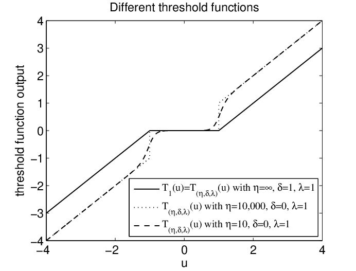
Where the value of $\lambda$ still denotes the threshold, the $\eta$ is a parameter to control the speed of the threshold transition, and $\delta\in[0,1]$ indicates what fraction of an additive adjustment is made for values above threshold. Some examples of this general threshold function are provided in Fig.1. With this threshold function, a more general objective function can be solved, which is given by

Furthermore, for any $z_{i}=T_{(\eta,\delta,\lambda)}(u_{i})$, the relationship between $u_{i}$, $z_{i}$ and $\partial\psi_{(\eta,\delta,\lambda)}(z_{i})/\partial z_{i}$ is

Someone may want to construct the exact form of $\psi_{(\eta,\delta,\lambda)}(\cdot)$ but note that its analytical expression cannot be obtained generally. Nevertheless, this does not limit the application of the LCA because the neural dynamics are expressed in terms of the threshold function $T_{(\eta,\delta,\lambda)}(u_{i})$ rather than the exact penalty term. Setting $\eta\rightarrow\infty$, $\delta=0$ and $\lambda=1$, we obtain an ideal hard threshold function [23]:

Also, the corresponding penalty term is close to the $l_{0}$-norm component:

where $\mathcal{I}(\cdot)$ is an indicator function. Note that according to (II-D), the variables $z_{i}$ produced by the ideal threshold function cannot take values in the range of $[-1,0)$ and $(0,1]$. The details of (II-D) and (29) are provided in [23].

If we set $\eta\rightarrow\infty$ and $\delta=1$, then the general threshold function is reduced to the soft threshold function [23], given by

and the penalty term becomes the $l_{1}$-norm function:

The behavior of the dynamics under different settings has been studied in [23, 24, 27]. However, the limitation of LCA is that it can handle the unconstrained optimization problem only.

In the CLS method, the $l_{2}$-norm is used as its objective function, i.e., $\|\boldsymbol{\alpha}^{\mathrm{T}}{\boldsymbol{X}}\|^{2}_{2}$. It is well known that the $l_{2}$-norm works well in Gaussian noise environments, but is sensitive to outliers. In the presence of impulsive noise or outliers, the performance of model with $l_{p}$-norm ($p<2$) will outperform that with the $l_{2}$-norm. In this study, we focus on two particular $l_{p}$-norms, namely, $l_{1}$-norm and $l_{0}$-norm. The corresponding formulations are

and

To achieve the real-time solution, we use LPNN to solve the optimization problem (32) and (33). Prior to applying the LPNN framework, we need to resolve two issues. First, the inequality constraint in (32) and (33) should be convert to an equality, because the LPNN framework can only handle problems with equality constraints. Another issue is that the objective function in (32) and (33) are non-differentiable, while LPNN can only solve the problem with differentiable objective and constraints.

To deal with the first issue, we introduce a new variable $G$ into the inequality constraint to change it into an equality one, thus $B^{2}-4AC+G^{2}=\epsilon$ where $\epsilon$ is a small negative scalar ($\epsilon=-10^{-12}$ in our experiments). The formulations of (32) and (33) are then modified as

and

where

Based on the LCA approach, the second issue is resolved by considering the general form $\sum_{i=1}^{N}\psi_{(\eta,\delta,\lambda)}([\tilde{{\boldsymbol{X}}}^{\mathrm{T}}\tilde{\boldsymbol{\alpha}}]_{i})$ where $[\cdot]_{i}$ denotes the $i$th element of the vector. The problem in (34) or (35) becomes

When we set $\eta\rightarrow\infty$, $\delta=1$ and $\lambda=1$, (36a) is the $l_{1}$-norm objective function. On the other hand, the proximate $l_{0}$-norm expression is achieved by setting $\eta\rightarrow\infty$, $\delta=0$ and $\lambda=1$ in (36a).

To exploit the concept of LCA, we introduce the a dummy vector ${\boldsymbol{z}}=\tilde{{\boldsymbol{X}}}^{\mathrm{T}}\tilde{\boldsymbol{\alpha}}$. Then (36) becomes

According to (37) and the concept of LPNN, we first construct the following Lagrangian function:

In (38), $\tilde{\boldsymbol{\alpha}}$ and ${\boldsymbol{z}}$ are decision variable vectors while $\boldsymbol{\zeta}\in\mathbb{R}^{N}$, $\beta$ and $\gamma$ are the Lagrange multipliers. In the next step, we can use (38) to deduce the neural dynamics for the robust ellipse fitting problem given by (37). However, our preliminary experimental results find that the neural dynamics may not be stable. To improve the stability and convexity, several augmented terms are introduced into the objective function [17, 19, 20, 21, 22], then (37) becomes:

In (39), $C_{0}$, $C_{1}$ and $C_{2}$ are trade-off factors which are used for adjusting the magnitudes of the augmented terms. When they are large enough, the augmented terms will make the objective function of (39) be convex. But if they are too large, they may result in the dynamics converge to a local optimal solution. These three extra terms do not influence the objective function value at an equilibrium point. It is because at any equilibrium point, the constraints should be satisfied, i.e., ${\boldsymbol{z}}=\tilde{{\mathbf{X}}}^{\mathrm{T}}\tilde{\boldsymbol{\alpha}}$, $\tilde{\boldsymbol{\alpha}}^{\mathrm{T}}\mathbf{\Phi}\tilde{\boldsymbol{\alpha}}=1$, and $\tilde{\boldsymbol{\alpha}}^{\mathrm{T}}\mathbf{\Theta}\tilde{\boldsymbol{\alpha}}=\epsilon$. In other words, augmented terms will all equal zero at equilibrium point. Then the Lagrangian for (39) is:

For constructing neural dynamics, we need to calculate the gradient of Lagrangian (40) with respect to its decision variables and Lagrange variables. To handle the non-differentiable term, we utilize the concept of LCA, introduce an internal state variable ${\boldsymbol{u}}$ for ${\boldsymbol{z}}$ and the relationship between ${\boldsymbol{u}}$ and ${\boldsymbol{z}}$ is given by (23).

Now it is ready for us to define the dynamics, $(du_{i})/(dt)$, $i=1,\cdots,N$, and $(d\tilde{\boldsymbol{\alpha}})/(dt)$ for the state variables, and the dynamics, $(d\boldsymbol{\zeta})/(dt)$, $(d\beta)/(dt)$ and $(d\gamma)/(dt)$ for the Lagrangian variables. For the state variables $u_{i}$’s, we apply the LPNN and combine it with the LCA concepts, thus, their dynamics are

Based on (18a), the dynamics for the state variables in $\tilde{\boldsymbol{\alpha}}$ are given by

For the Lagrangian variables, their dynamics are obtained from (18b) as:

According to (40) and (25), the dynamics given by (41)–(45) become

It should be noticed that for the relationship given by (23), if the problem is formulated using the $l_{0}$-norm objective, we should set $\eta$ as a large number, $\delta=0$ and $\lambda=1$. While, if the problem uses the $l_{1}$-norm objective function, we should set $\eta=\infty$, $\delta=1$ and $\lambda=1$.

In the LPNN approach, the circuit complexity depends on the time derivative calculations. From (46)–(50), the most computationally demanding step is to determine the product of a $N\times 7$ matrix and $7\times 1$ vector. Hence the complexity to obtain the time derivatives is equal to ${\cal O}(N)$ only.

In simulation, we can update (46)–(50) as rules:

where ^(k) corresponds to the estimate at the $k$th iteration and $\mu>0$ is the step size which should not be too large to avoid the divergence. Upon convergence of the iterative procedure, we obtain the estimate of $\tilde{\boldsymbol{\alpha}}$, denoted by $\tilde{\boldsymbol{\alpha}}^{\ast}$. From $\tilde{\boldsymbol{\alpha}}^{\ast}$, the ellipse parameter estimates $\{a^{\ast},b^{\ast},c^{\ast}_{x},c^{\ast}_{y},\theta^{\ast}\}$ are then computed from:

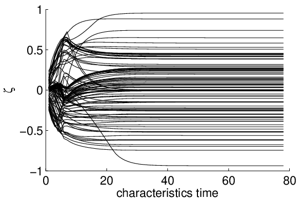
Fig. 2 shows the dynamics of the estimated parameters in a typical experiment. The settings are described in Section V.B. It is seen that the network can settle down within 40 characteristic times.

References

- [1] N. Chernov and G. Ososkov, “Effective algorithms for circle fitting,” Computer Physics Communications, vol. 33, no. 4, pp. 329–333, 1984.
- [2] K. Paton, “Conic sections in chromosome analysis,” Pattern Recognition, vol. 2, no. 1, pp. 39–51, 1970.
- [3] R. O. Duda and P. E. Hart, “Use of the Hough transformation to detect lines and curves in pictures,” Communications of the ACM, vol. 15, no. 1, pp. 11–15, 1972.
- [4] D. H. Ballard, “Generalizing the Hough transform to detect arbitrary shapes,” Pattern Recognition, vol. 13, no. 2, pp. 111–122, 1981.
- [5] D. Barwick, “Very fast best-fit circular and elliptical boundaries by chord data,” IEEE Transactions on Pattern Analysis and Machine Intelligence, vol. 31, no. 6, pp. 1147–1152, Jun. 2009.
- [6] Y. Nakagawa and A. Rosenfeld, “A note on polygonal and elliptical approximation of mechanical parts,” Pattern Recognition, vol. 11, no. 2, pp. 133–142, 1979.
- [7] P. L. Rosin and G. A. West, “Nonparametric segmentation of curves into various representations,” IEEE Transactions on Pattern Analysis and Machine Intelligence, no. 12, pp. 1140–1153, 1995.
- [8] S. J. Ahn, W. Rauh, and H.-J. Warnecke, “Least-squares orthogonal distances fitting of circle, sphere, ellipse, hyperbola, and parabola,” Pattern Recognition, vol. 34, no. 12, pp. 2283–2303, 2001.
- [9] P. L. Rosin, “A note on the least squares fitting of ellipses,” Pattern Recognition Letters, vol. 14, no. 10, pp. 799–808, 1993.
- [10] E. S. Maini, “Enhanced direct least square fitting of ellipses,” International Journal of Pattern Recognition and Artificial Intelligence, vol. 20, no. 6, pp. 939–953, 2006.
- [11] F. L. Bookstein, “Fitting conic sections to scattered data,” Computer Graphics and Image Processing, vol. 9, no. 1, pp. 56–71, 1979.
- [12] K. Kanatani, “Statistical bias of conic fitting and renormalization,” IEEE Transactions on Pattern Analysis and Machine Intelligence, no. 3, pp. 320–326, 1994.
- [13] P. D. Sampson, “Fitting conic sections to “very scattered” data: An iterative refinement of the Bookstein algorithm,” Computer Graphics and Image Processing, vol. 18, no. 1, pp. 97–108, 1982.
- [14] W. Gander, G. H. Golub, and R. Strebel, “Least-squares fitting of circles and ellipses,” BIT Numerical Mathematics, vol. 34, no. 4, pp. 558–578, 1994.
- [15] J. Liang, M. Zhang, D. Liu, X. Zeng, O. Ojowu, K. Zhao, Z. Li, and H. Liu, “Robust ellipse fitting based on sparse combination of data points,” IEEE Transactions on Image Processing, vol. 22, no. 6, pp. 2207–2218, Jun. 2013.
- [16] J. Liang, Y. Wang, and X. Zeng, “Robust ellipse fitting via half-quadratic and semidefinite relaxation optimization,” IEEE Transactions on Image Processing, vol. 24, no. 11, pp. 4276–4286, 2015.
- [17] S. Zhang and A. Constantinides, “Lagrange programming neural networks,” IEEE Transactions on Circuits and Systems II: Analog and Digital Signal Processing, vol. 39, no. 7, pp. 441–452, 1992.
- [18] M. Nagamatu and T. Yanaru, “On the stability of Lagrange programming neural networks for satisfiability problems of prepositional calculus,” Neurocomputing, vol. 13, no. 2, pp. 119–133, 1996.
- [19] X. Zhu, S.-W. Zhang, and A. G. Constantinides, “Lagrange neural networks for linear programming,” J. Parallel Distrib. Comput., vol. 14, no. 3, pp. 354–360, Mar. 1992.
- [20] V. Sharma, R. Jha, and R. Naresh, “An augmented Lagrange programming optimization neural network for short term hydroelectric generation scheduling,” Engineering Optimization, vol. 37, pp. 479–497, Jul. 2005.
- [21] J. Liang, H. C. So, C. S. Leung, J. Li, and A. Farina, “Waveform design with unit modulus and spectral shape constraints via Lagrange programming neural network,” IEEE Journal of Selected Topics in Signal Processing, vol. 9, no. 8, pp. 1377–1386, 2015.
- [22] J. Liang, C. S. Leung, and H. C. So, “Lagrange programming neural network approach for target localization in distributed MIMO radar,” IEEE Trans. Signal Process., vol. 64, no. 6, pp. 1574–1585, Mar. 2016.
- [23] C. J. Rozell, D. H. Johnson, R. G. Baraniuk, and B. A. Olshausen, “Sparse coding via thresholding and local competition in neural circuits,” Neural Computation, vol. 20, no. 10, pp. 2526–2563, 2008.
- [24] A. Balavoine, J. Romberg, and C. J. Rozell, “Convergence and rate analysis of neural networks for sparse approximation,” IEEE Transactions on Neural Networks and Learning Systems, vol. 23, no. 9, pp. 1377–1389, 2012.
- [25] D. Liu and J. Liang, “A Bayesian approach to diameter estimation in the diameter control system of silicon single crystal growth,” IEEE Transactions on Instrumentation and Measurement, vol. 60, no. 4, pp. 1307–1315, Apr. 2011.
- [26] A. Fitzgibbon, M. Pilu, and R. Fisher, “Direct least square fitting of ellipses,” IEEE Transactions on Pattern Analysis and Machine Intelligence, vol. 21, no. 5, pp. 476–480, 1999.
- [27] A. Balavoine, C. J. Rozell, and J. Romberg, “Global convergence of the locally competitive algorithm,” in Proc. IEEE Digital Signal Processing Workshop and IEEE Signal Processing Education Workshop (DSP/SPE), 2011, pp. 431–436.
- [28] J. Muñoz-Pérez, O. de Cózar-Macías, E. Blázquez-Parra, and I. L. de Guevara-López, “Multicriteria robust fitting of elliptical primitives,” Journal of Mathematical Imaging and Vision, vol. 49, no. 2, pp. 492–509, 2014.