UAI-PHY-18/01
Black hole and BTZ-black string in the Einstein- Skyrme model
Abstract
We present novel analytic hairy black holes with a flat base manifold in the (3+1)-dimensional Einstein -Skyrme system with negative cosmological constant. We also construct (3+1)-dimensional black strings in the Einstein -non linear sigma model theory with negative cosmological constant. The geometry of these black strings is a three-dimensional charged BTZ black hole times a line, without any warp factor. The thermodynamics of these configurations (and its dependence on the discrete hairy parameter) is analyzed in details. A very rich phase diagram emerges.
pacs
04.20.Jb, 04.40.-b, 04.40.Nr, 04.70.BwI Introduction
The idea that one can make up fermions out of a purely Bosonic Lagrangian as solitonic excitations (for a detailed review see [1]) is one of the most remarkable results in Quantum Field Theory (QFT henceforth). Skyrme’s theory [2] is the most important example in nuclear and particles physics. When the Skyrme term is included in the low energy action of Pions, static soliton solutions with finite energy, called Skyrmions (see [3]-[6]) describing Fermionic degrees of freedom are allowed (see [7]-[15] and references therein). The agreement of the theoretical calculations with experiments is quite good. However, the Skyrme field equations are very difficult to solve (one reason being that the Skyrme-BPS bound cannot be saturated in the generic case) and so, until very recently, basically no analytic solution of the Skyrme field equations in which one could analyze explicitly the effects of the Skyrme term was available.
Due to the close relation of the Skyrme theory with the low-energy limit of QCD, the Einstein-Skyrme system has attracted a lot of attention. The first important results in this topic were constructed numerically. In particular, Droz, Heusler, and Straumann [16] (following the findings of Luckock and Moss [17]) constructed black hole solutions with a non-trivial Skyrme hair with a spherically symmetric ansatz. Such counterexample to the no-hair conjecture is also stable against linear perturbations [18]. In [19] and [20] gravitating solitons and their dynamical features have been also considered.
When the Skyrme coupling constant vanishes, the Skyrme action reduces to the nonlinear sigma model, which is a very important effective field theory in itself. The applications of the nonlinear sigma model range from quantum field theory to statistical mechanics systems, to the quantum hall effect, to super fluid 3He and string theory [21]. The main use for the nonlinear sigma model is, probably, the description of the low-energy dynamics of Pions (see for instance [22], or for a detailed review [23]). Therefore, the Einstein nonlinear sigma model system is also a very important topic, and the construction of analytical solutions is as relevant as the Einstein-Skyrme system itself, since in the same way, until recently only numerical solutions had been found11 1 If a suitable interaction potential is included, some interesting analytic solutions can be constructed [46]..
It is worth to emphasize that the search for analytic solutions in models such as the Skyrme model, the nonlinear sigma model and their gravitating counterparts is not just of academic interest. For instance it was a well known fact, from a numerical point of view, that the Skyrmions in flat spaces becomes unstable, when a too large isospin chemical potential is introduced. But only only very recently, in [24] and [25], it was derived an analytic formula for this critical chemical potential which also clarifies the physical mechanism behind this instability. The hope is that these techniques, which lead to such important step in the analysis of the Skyrme phase diagram on flat spaces, will also be useful in clarifying the phase diagrams of hairy black holes in the Einstein-Skyrme system, as well as in the Einstein-nonlinear sigma model system. Besides the intrinsic interest of these phase diagrams, the hairy black holes and black strings solutions which will be constructed here have potentially many applications in the context of AdS/CFT correspondence (see [26], [27] and references therein).
Using some recent results on the generalization of the hedgehog ansatz to non-spherically symmetric configurations 22 2 The techniques developed in these references are very flexible as they apply to the Skyrme model (both without and with extra moduli degrees of freedom), to the Skyrme-Einstein system as well as to the Yang-Mills-Higgs theory. [28]-[43]33 3 Similar solutions but in different theories have been found in [44] and [45] , we construct analytic black holes with flat horizons possessing a discrete hairy parameters: to the best of authors knowledge, these are the first examples of this type in Einstein-Skyrme theory. The thermodynamics of these black holes is analyzed in details and a very rich phase diagram is disclosed.
The same techniques also allow to construct black strings in the (3+1)-dimensional Einstein nonlinear sigma model theory with negative cosmological constant: the (2+1)-dimensional transversal sections of these black strings correspond to a charged BTZ black hole. The novel feature of these black strings is that (unlike what happens, for instance, in the BTZ black string constructed in [47]) the present charged BTZ black string has no warping factor as the metric is really the direct product of a charged BTZ with a line.
In the following section we review the Einstein-Skyrme and Einstein nonlinear sigma model systems. In Sec. III, a pedagogical overview of the generalized hedgehog ansatz is presented and the matter field and metric ansatz are constructed. In Sec. IV, the field equations and the solutions for some interesting cases are shown. In Sec. V, thermodynamics and stability of our solutions is discussed. Concluding remarks and future prospects are summarized in the last section. Some useful formulas are collected in the appendix.
II The Einstein - Skyrme and Einstein - Nonlinear sigma model systems
The Skyrme Lagrangian describes the low-energy interactions of pions or baryons. This observation of Skyrme was, and still is, remarkable because it provided with the first example of a purely Bosonic Lagrangian able to describe both bosonic and Fermionic degrees of freedom. The Skyrme field is a -valued scalar field described by the following action
| (1) |
where the gravitational action and the Skyrme action are given by
| (2) | ||||
| (3) |
Here and are defined by
| (4) | ||||
| (5) |
while is the Newton constant and the positive parameters and are fixed by comparison with experimental data. The Skyrme fields satisfy physically reasonable reasonable condition, such as the dominant energy condition [48].
For convenience, defining and , we write the Skyrme action as
| (6) |
The nonlinear sigma model corresponds to the limit of the above action. The resulting Einstein equations are
| (7) |
where is the Einstein tensor and
| (8) |
The Skyrme equations are written as
| (9) |
Hence, the full Einstein-sigma model field equations correspond to the limit in Eqs. (7), (8) and (9).
The winding number for a given solution is given by
| (10) |
It is well known (see, for instance, [21] and references therein) that the above integral is a conserved topological charge of the theory. When the topological density is integrated on a space-like surface, is the Baryon number of the configuration.
Here is expressed as
| (11) |
in the basis of the SU(2) algebra generators
(where are the Pauli matrices, the Latin index corresponds to the group index, which is raised and lowered with the flat metric ), which identically satisfy
| (12) |
where is the identity matrix and and are the totally antisymmetric Levi-Civita symbols with .
The standard parametrization of the SU(2)-valued scalar :
| (13) |
where and satisfy
| (14) |
Thus, as expected in the case, the theory describes three scalar degrees of freedom (due to the constraint in Eq. (14)). From the definition (4), is written as
| (15) |
Another convenient way (which will be used in the following) to describe -valued scalar field uses the Euler angle representation (for a detailed review see [49]). In this representation, the most general -valued scalar field can be written as
| (16) |
As it happens in the standard representation for -valued scalar field (in Eqs. (13) and (14)), in the Euler angle representation44 4 If necessary, one can pass from one representation to the other (as it is a standard computation to express , and in terms of the and in Eqs. (13) and (14) using, for instance, the results in [49]). However, the novel results presented here are more easily expressed in the Euler angle representation. in Eq. (16) there are three scalar degrees of freedom: the three scalar functions , and . Thus, in order to solve the Skyrme field equations in the Euler angle representation one needs to construct a good ansatz for , and : we will outline the strategy to build such an ansatz in the next section.
III Matter field and metric ansatz
A very important class of black holes both from the strictly theoretical viewpoint as well as from the point of view of holographic applications corresponds to hairy black holes with flat horizons and negative cosmological constant (see [26], [27] and references therein). The interest in black holes with hairy parameters arises from the fact that often such black holes exhibit a very complex thermodynamical behavior. The interest in having flat horizons with negative cosmological constant lies in the possibility to describe, via the AdS/CFT correspondence, very interesting field theories on the boundary of the black hole space-time itself. It is usually quite difficult to construct hairy black holes in sectors of the standard model minimally coupled with General Relativity. These considerations are behind our interest in constructing this type of configurations within the Einstein-Skyrme system as it describes the minimal coupling of (the low energy limit of) QCD with General Relativity.
III.1 The main theoretical tool: the generalized hedgehog ansatz
In this subsection, the concept of hedgehog ansatz in the Einstein-Skyrme system will be shortly described. The technical difficulty to construct analytic black hole configurations in the Einstein-Skyrme system arises from the fact that already the Skyrme field equations on flat space-times in themselves are a very difficult nut to crack (see [4] and references therein). Thus, one may argue that the situation in the coupled Einstein-Skyrme system is even worse. In fact, quite recently an effective strategy suitable to deal with this type of problems has been developed in the references [28]-[43]. Such a strategy is divided into two steps.
The first step: identify the symmetries of the space-times of interest in such a way to distinguish clearly the Killing coordinates from the non-Killing coordinates of the metric.
The second step: choose the valued ansatz in such a way that it also depends on the Killing coordinates of the metric55 5 It is worth to emphasize that, in the simple case of one scalar field (without internal symmetries) minimally coupled with general relativity, this is not what one would do. Consider, for instance, a static spherically symmetric space-time. The most obvious ansatz for the scalar field would be to assume that the scalar field only depends on the (non-Killing) radial coordinate. of interest with the additional (very important) condition
| (17) |
where is the Lie derivative along the Killing fields (denoted by ) of the metric while is the energy-momentum tensor (defined in Eq. (8)) corresponding to the valued ansatz itself. The possibility to implement the above strategy arises from the non-trivial internal symmetry group of the field theory minimally coupled with gravity.
The requirement in Eq. (17) asks to find an ansatz which is not invariant under the symmetries of the metric but which, nevertheless, possesses an energy-momentum tensor which is compatible with the symmetries of the space-time of interest. Such a condition is somehow rigid since often it allows to determine the functional form of the ansatz itself almost completely.
Once Eq. (17) has been satisfied, it is usually a quite easy task to verify whether or not there is still enough freedom left in to be able to solve (at least numerically) the Skyrme field equations in the metric of interest.
Thus, the above two steps (and in particular Eq. (17)) summarize the generalized hedgehog ansatz.
The word ”generalized” arises from the following fact. In the original papers by Skyrme [2], the spherically symmetric hedgehog ansatz was
| (18) | ||||
| (19) | ||||
| (20) |
where is the so-called Skyrmion profile. Although Skyrme arrived at his ansatz following a different reasoning, it is a direct computation to verify that the ansatz in Eqs. (18) and (20) satisfies Eq. (17) in which the Killing fields correspond to the rotations of the flat metric in Eq. (19). In other words, the Skyrme ansatz could have been found solving Eq. (17) in a spherically symmetric metric in which the Killing fields correspond to the rotations. Once the functional form of the ansatz has been restricted by Eq. (17), one can plug in it into the three Skyrme field equations Eq. (9) corresponding to the metric with the Killing fields . In the original case analyzed by Skyrme, it can be directly verified that when one plugs Eqs. (18) and (20) into Eq. (9) (for the metric in Eq. (19)) the three Skyrme field equations become proportional, so that the full system of three coupled field equations reduces to just one scalar equation for the Skyrmion profile .
All the above very convenient properties of the original spherical hedgehog ansatz are well known of course. However, what was not widely appreciated in the literature is that one can construct ansatz with similar nice properties even without spherical symmetry. The key point is that the condition in Eq. (17) makes sense in more general situations than spherically symmetric space-time. Indeed, this simple observation in [28] [29] allowed to find the first non-trivial analytic solutions in Skyrme and Einstein-Skyrme theories in [30] [31] [35] [24] [25]. These are the reasons behind the name generalized hedgehog ansatz.
In the present case, there is an additional technical problem. We are interested in hairy black holes, thus we look for configurations possessing neither topological nor Noether charges related with the isospin symmetry. This issue will be analyzed in the next subsection.
III.1.1 An example
Before going into the details of the novel results, here we will describe an example (which corresponds to the first analytic gravitating Skyrmions in (3+1)-dimensional Einstein-Skyrme system found in [35]) in which the strategy outlined above works perfectly. Let us consider the following space-time metric (the first step of the strategy)
| (21) |
| (22) |
The spatial sections of the above metric are three-spheres. Consequently, the above metric possesses all the Killing fields of the three-sphere (and , and can be considered to be Killing coordinates). The only non-trivial ”non-Killing” coordinate is the time .
The second step of the strategy corresponds to find an ansatz of such that
where are the Killing field of the three-sphere. The solution to the above condition is given by
| (23) | ||||
where
| (24) |
As it has been already emphasized, at a first glance the situation is quite dangerous since the condition in Eq. (17) is rather rigid as, in this example, it fixes the ansatz for the -valued scalar field completely while the Skyrme field equations have not been considered yet! Nevertheless, remarkably (as it was shown in [35]), when one plugs the ansatz in Eqs. (23) and (24) into the Skyrme field equations in Eq. (9) in the metric in Eq. (21), the Skyrme field equations are identically satisfied. Thus, despite the fact that the condition in Eq. (17) gives rise to an ansatz in which, basically, there is no freedom left, the resulting ansatz is very well suited to solve the Skyrme field equations. Thus, we are only left with the problem to solve the Einstein equation with the energy-momentum tensor in Eq. (8) corresponding to the ansatz in Eqs. (23) and (24). In fact, the generalized hedgehog strategy has been designed in such a way that this last step is compatible: the condition precisely ensures that the resulting energy-momentum tensor is a consistent source for the metric in Eq. (21). A direct computation shows [35] that the Einstein-Skyrme equations reduce66 6 Note that these equations corresponds to the ones in reference [35] by rescaling . in this example to
| (25) |
where denotes derivative with respect to the time coordinate, . In the following sections, it will be shown that this strategy works very well even when the metric of interest has different symmetries.
III.2 The concrete ansatz for the novel solutions
The first step of the generalized hedgehog strategy is to identify the symmetries of the class of metric of interest. In the present case, the natural metric ansatz describing both black holes with flat horizons and black strings is
| (26) |
where the range of the angular coordinates can be fixed as
| (27) |
The second step requires to solve Eq. (17) for a valued scalar field which also depend on the Killing coordinates and of the metric in Eq. (26). Form the viewpoint of the generalized hedgehog approach, the simplest possibility is actually to search for an ansatz which only depends on such Killing coordinates and . As it will be now shown, this approach does lead to novel and interesting solutions. A further motivation behind this choice is that we are interested in black holes with hairy parameters. These configuration are easier to identify in case of absence of extra parameters related to topological or Noether charges coming from the symmetry of the matter field. The simplest way to avoid the presence of a non-vanishing topological charge is to allow the matter field to only depend on two coordinates (which, according to the generalized hedgehog strategy, should then be Killing coordinates) as in this case in Eq. (10) vanishes identically.
In the cases in which the Killing fields of the metric of interest are commuting (as for the metric in Eq. (26)) it is more convenient to use the Euler angle representation in Eq. (16). The simplest non-trivial possibility is
| (28) |
with two real functions of the Killing coordinates and so that, obviously, one has
where
It is worth to emphasize here that the ansatz in Eq. (28) does not possess Noether charges associated to the internal symmetry group of the theory (the global Isospin group in the present case). The reason is that such a Noether charge would be the spatial integral of the time-component of the corresponding Noether current. On the other hand, the time-component of the Noether current is proportional to
so that it vanishes identically since the configuration is static. Hence, the ansatz for the scalar field we will consider here does carry neither topological nor Noether charges.
The (second part of the) second step of the strategy is now to solve the following equation
in which is the energy-momentum tensor (defined in Eq. (8)) corresponding to the ansatz in Eq. (28) and to the metric in Eq. (26). The solution to the above condition is given by and . In matrix form, this solution corresponds to the following :
| (29) |
Once again, as it also occurred in the example described in the previous subsection, the ansatz produced by the present strategy is quite rigid and, in this case, only two integration constants ( and ) are left.
Nevertheless, also in this case a direct computation reveals that the Skyrme field equations Eq. (9) with the ansatz in Eqs. (28) and (29) are identically satisfied in any metric of the form in Eq. (26). This is the big technical achievement of the generalized hedgehog strategy developed in [28]-[43]: it allows to reduce the full Einstein-Skyrme system just to the Einstein equations with the energy-momentum tensor of the Skyrme field (as the Skyrme field equations, which usually are the difficult part of the problem, are identically satisfied). Moreover, by construction, the energy-momentum tensor is compatible with the symmetries of the metric of interest (due to Eq. (17)).
III.2.1 The topology of the horizon
In this article we will be mainly interested in compact horizons, therefore we need to impose (anti)periodic boundary conditions for the Skyrme field (see [4], [12]), that is, any solution of the form in Eq. (29) of the Skyrme field equations in the metric Eq. (26) must satisfy
with , integers. In order to have a well defined the integration constants must be integers numbers77 7 In principle, one can choose a different range for the coordinates to rescale these values with the metric functions and coordinate definitions. Nevertheless, being integrating constant of the matter field, the parameters cannot be completely reabsorbed from the solution. We leave them explicitly to better understand their physical role and relevance, as we see below.,
| (30) |
These parameters, as can be seen from (29), are related to
number of coverings of the group.
The angles identifications
we are considering determines not only the topology of the event horizon but
also the global topology of the spacetime, even in the asymptotic region. This
means that even though the metric, for large values of the radial coordinate,
behaves locally as the Anti-de-Sitter space, as can be easily seen from the
curvature tensors, the asymptotic region does not recover globally the full
spacetime. Therefore when the radial coordinate goes to infinity the
spacetime we are studying here are only asymptotically locally
Anti-de-Sitter.
The great physical interest of these configurations is
that they show very clearly that the Skyrme contribution to the action is
quite relevant even for purely Pionic configurations without Baryon charge.
For instance, as it will be shown below, it gives rise to a black hole metric
with a -term which mimics the presence of a Maxwell source.
IV Analytical solutions
In the previous section we have reduced consistently the full Einstein-Skyrme system for the metric in Eq. (26) and the Skyrme ansatz in Eqs. (28) and (29) to the Einstein equations with the Skyrme energy-momentum tensor corresponding to the ansatz in Eqs. (28) and (29). In principle there are four coupled nonlinear differential equations (see Appendix A), but it is possible to show that one of these is a combination of the others because of the Bianchi’s identity and the form of the metric ansatz for the matter field. In this section we show some relevant cases where it is possible to integrate the system analytically. In what follows we will consider and .
IV.1 Hairy Black hole
If we take and , the field equations leads to
where is an integration constant. The metric
| (31) | ||||
represents a hairy black hole with flat horizon. This solution reduce to the black hole of [43] when , while it is the natural flat horizon generalization of the spherical metric found in [29]. Black hole with flat horizons are especially relevant in view of their holographic applications (see, for instance, [47]). For there is only one real root for the function which corresponds to the event horizon
| (32) |
For , the roots of can also be found analytically, but they are more involved than the ones of (32), because the algebraic equation becomes of fourth order, thus is more instructive to draw them as function of the mass parameter as in Figure 1.

Interestingly enough, as is shown in the figure, neither the mass
of the black hole nor the event horizon radius can be arbitrarily small
because the event horizon is not defined for small masses, unlikely the
standard general relativity case.
Even in the case, where
there is only one killing horizon, from Eq. (32) one infers that the
mass parameter should satisfy in order the square root to be real. Therefore, the
event horizon cannot be arbitrarily small either but, for the extremal value
of the mass parameter, which saturate the previous inequality, it can be
reduce at most to .
This latter feature of the parameter resemble the electric charge of
the Reissner-Nordstrom solution, but, in the Skyrme case, the parameters
must be quantized due to the boundary conditions satisfied by the
Skyrme field. In particular, plays the role of a discrete hairy
parameter (since, as we observed in the previous section, the Skyrme
configurations in Eq. (29) possess neither Noether charges nor
topological charges). According to this picture the hair cannot be considered
neither of a primary type, because it cannot variate continuously, nor
secondary type because it is not completely fixed. We might consider it
belonging to an intermediate class; a sort of semi-primary hair.
The non-removability of resembles, to some extent, the role
played by the mass parameter of the three-dimensional BTZ black hole
[50]: in that case, once the azimuthal coordinate is fixed, it cannot be
reabsorbed by a coordinate transformation to get global AdS space-time.
Moreover, in the next section, we will show how the thermodynamics potentials
depends crucially on the hair parameters.
Depending on the
identifications of the coordinates (), the base manifold can be
considered open or compact. When the extremal points of the range of
() are identified, the base manifold becomes a topological torus
with area . In that case the ratio determines
the geometry of the toroidal base manifold, being its
Teichmuller parameter. Therefore, the discrete parameters and
can be reabsorbed by rescaling properly the coordinates and the integration
constants only at the price of deforming the geometry of the base manifold and
the Skyrmionic field.
The spacial infinity region is asymptotically
locally AdS.
When the Skyrmionic parameters coincide, ,
one can take the limit . In that case the contribution of
the matter field vanishes and the pure gravitational black hole solution of
[51] is recovered.
IV.2 Charged-like BTZ-black string
When we choose and (with an arbitrary constant), the Einstein equations are satisfied only in the sector , and leads to
In the case in which the cosmological constant is negative and the integration constant , the resulting metric reads
| (33) | ||||
This solution corresponds to a black string with one compactified direction
(namely ) whose compactification radius has been fixed by the field equations. The
three-dimensional metric (corresponding to the hypersurfaces)
resemble the charged BTZ black holes [52] with mass
and square charge .
The nonlinear sigma model
induce an effective electric charge in the three-dimensional metric defining
the black string. It is worth to note that, unlike what happens for instance
in the BTZ black string constructed in [47], the present charged BTZ
black string has no warping factor, as the metric is really the direct product
of a charged BTZ with a one-dimensional line (which can be also considered
compatified in a circle). It is also worth to note that it is not
possible to turn off the nonlinear sigma model, to obtain a pure gravitational
solution, as the factor would be singular. Thus, the parameter
plays the role of an effective electric charge while the parameter
determines the size of the compactified direction of the black string.
As the great majority of charged black holes, this string posses, in general,
both a inner and outer horizon . Unfortunately, due to the presence
of the transcendental function in , the position of the horizon cannot
be written with elementary functions, but only through the
Lambert- function (also known as the ProductLog function) in this
way
| (34) | ||||
| (35) |
As can be seen from the Figure 2, as in the previous subsection black hole case, the event horizon cannot vanish, as it happens in the pure gravity case. In the presence of the Skyrmionic matter , depending on the values of the parameter , can only reach a positive minimum value.

V Thermodynamics
A very interesting topic is the proper dynamical stability analysis of the present black holes and black strings solutions. The main difficulty is revealed by a direct computation of the fully coupled linearized Einstein-Skyrme field equations in the black hole and black string background solutions. When the Skyrme field equations are taken into account (due to their matrix-valued and non-linear nature), the linearized field equations cannot be reduced to a single master Schrodinger-like equation for the perturbations (unlike what happens in many situations without matter fields). This fact prevents any analytic attempt to analyze dynamical stability. Thus, one has to solve numerically the matrix-valued linearized field equations around the black hole and black string background solutions. However, this point is very difficult even from the numerical point of view and it requires suitable generalizations of the methods available in the literature. We hope to come back on this issue in a future publication.
On the other hand, as it is well known, the analysis of thermodynamics of black holes and black strings solutions (besides to be very interesting in itself) provides with very good qualitative indications on the possible appearance of instabilities. Thus, in this section we study the thermodynamic of these solutions and also perform a thermodynamical stability analysis through comparison between the thermodynamic potentials.
V.1 Mass, temperature and entropy
The Hawking temperature, related to the surface gravity , is given by
| (36) |
where is the timelike killing vector . From the Bekenstein-Hawking formula, we can take the entropy as a quarter of the area
| (37) |
To compute the mass will use the standard ADM result, as in [53]. Consider as the two-dimensional spacelike surface at spatial radial infinity at constant time. The radial orthonormal vector to is given by , the extrinsic curvature of is given by , and its trace is computed with the two dimensional metric of the base manifold : . The Hamiltonian mass is then given by
| (38) |
where is the trace of the extrinsic curvature of
embedded in the background reference space-time.
As
pionic background, for the two solutions, the metrics (31) and
(33), with the vanishing mass parameters and , are chosen.
It is worth to point that the mass can also be computed within the phase space
formalism [54]-[55], giving the same result. Recently these
results have been also confirmed, thanks to counterterms methods
[43], for similar matter.
For the black hole solution,
using the above prescriptions we can compute the temperature, entropy and
mass. In terms of the event horizon we have, respectively
| (39) | ||||
| (40) | ||||
| (41) | ||||
| (42) |
while, for the black string with horizon radius , we obtain
| (43) | ||||
| (44) | ||||
| (45) |
In both cases these quantities satisfy the first law of black hole thermodynamics
| (46) |
V.2 Thermodynamical stability analysis
From the analysis of the heat capacity, defined as
| (47) |
we can infer the local thermodynamic stability of the two solutions. Written it terms of the event horizon radius, and for the black hole and the black string respectively, it reads
| (48) |
and
| (49) |
The stability under thermal fluctuation occurs when the sign of the heat capacity is positive, which means for the black hole and black string solutions
| (50) | ||||
| (51) |
These two values coincides, when the Skyrme coupling constant
vanishes. Note that the above inequalities (50) and (51)
are automatically satisfied for both the black hole and black string event
horizons.
One might wonder if the black string might be affected by a
Gregory-Laflamme instability, where the string may collapse in a line of black
holes [56]-[57].
Unfortunately, due to the complexity of the field equations, for linear perturbations, the system can not be uncoupled to obtain a master equation for one of the components of the perturbation; therefore it is not possible to integrate numerically the system in the Gregory-Laflamme form and study the unstable modes of the solutions. However, it is possible to analyze the stability and phase transitions from the thermodynamic point of view.
A necessary condition for this phenomena to occur, as proposed in [58], is the negativity of the quantity
but in the regions of thermodynamic local stability of the string, such as the
one described by (51), it can not happen.
In fact, from the
inspection of the entropies of the two solutions at equal mass, we further
confirm the absence of the Gregory-Laflamme instability in our setting. More
specifically, from Eq. (42) and (45), we can impose the equal
mass constraint to express and plot both, the black hole and
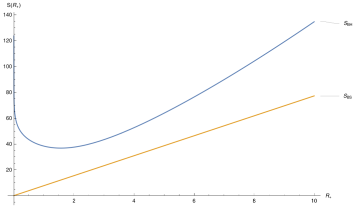
black string entropy at equal mass as a function of . As shown in
Figure 3, instability is not likely to occur because the
black hole entropy, at equal mass and Skyrme parameters , is always
bigger than the black string one.
Some further indication of the thermodynamic stability may come from the study of the free energies of the two solutions. Thus, we consider the free energy of the black hole and of the black string, which in terms of their event horizon are, respectively
| (52) | ||||
| (53) |
To obtain the free energy in terms of the temperature is sufficient to invert Eqs. (39) and (43), take the only positive root to get and ) and substitute respectively into (52) and (53). The resulting analytical expression of the free energy as a function of the temperature is a little cumbersome. Thus, is more significant to draw some picture of the free energy for some fixed values of the parameters to appreciate, in particular, the dependence with respect to the parameter , as can be seen in Figure 4 and Figure 5.


We recall that represent the vacuum solution for the black hole
case. Configurations with bigger values of are thermodynamically
favoured (as embodied, for instance, by and in Figure
4) with respect to the pure gravitational solution because the
free energy is lower. The situation can change for different values of the
for the black hole case. In particular, as can be seen in the above
graphs, there are critical values of the temperature, depending on the values
of the parameters, where free energies of two different configurations
intersect, thus phase transition might be expected if discrete
variations are allowed. The same qualitative behavior can be read from the
graph of the black string, but one have to remember that in this case the
comparison with the vacuum solution is not possible because proper black
string in pure general relativity without matter are not known.
VI Summary and perspectives
In this paper we have constructed the first examples, to the best of authors knowledge, of analytic hairy black holes with a flat toroidal horizons in the (3+1)-dimensional Einstein -Skyrme system with negative cosmological constant. The periodic boundary conditions satisfied by the Skyrme configurations introduce a discrete hairy parameter (as these black hole solutions possess neither topological nor Noether charges). Such hairy parameter can be considered neither primary (since it does not vary continuously) nor secondary (since it can vary in a discrete set). The solution is asymptotically locally AdS. The thermodynamics of the hairy black hole has been analyzed in detail. The behavior one obtains is qualitatively similar to the recent results found numerically in [59] in a different context.
Using similar techniques, we have constructed a black string in the (3+1)-dimensional Einstein non-linear sigma model theory with negative cosmological constant. The (2+1)-dimensional transversal sections of these black strings correspond to a charged BTZ black hole. In this case the role of the electromagnetic field is played by the pionic coupling constant. These configurations can be considered as a proper black string since there is no warping factor.
The exact hairy black hole solutions with flat horizons constructed here have potentially applications in the context of the AdS/CFT correspondence (see [26] and references therein). We hope to analyze in more details these applications in a future publication.
Another very interesting topic is the dynamical stability analysis of the present black holes and black strings solutions. As it has been explained in the previous sections, this point is very difficult even from the numerical point of view. The main issue is related to the fact that, when the Skyrme field equations are taken into account, the fully coupled linearized Einstein-Skyrme system cannot be reduced to a single master Schrodinger-like equation for the perturbations as the linearized field equations do not decouple (unlike what happens in many situations without matter fields). Thus, one has to solve (numerically) a system of (at least) tree coupled differential equations. We hope to come back on this issue in a future publication.
Acknowledgements
The authors are grateful to Julio Oliva for many enlightening comments. M.L. and A.V. appreciates the support of CONICYT Fellowship 21141229 and 21151067, respectively. This work has been funded by the Fondecyt grants 1160137 (FC) and 11160945 (M.A.). M.A. is supported by Conicyt - PAI grant no 79150061 . The Centro de Estudios Científicos (CECS) is funded by the Chilean Government through the Centers of Excellence Base Financing Program of Conicyt.
VII Appendix
VII.1 Main field equations
The coupled nonlinear differential equations of the Einstein-Skyrme system for , , and are given by
| (54) | ||||
| (55) | ||||
| (56) | ||||
| (57) |
VII.2 Gravitating regular solution
If we choose in the field equations and integrate the system, the following relations
| (58) |
reduces the system to a single equation, that can be easily solved to obtain
| (59) |
with , integration constants. This metric have no curvature singularity and represents a four-dimensional space-time that is the product of two two-dimensional space-times with constant curvature; namely .
References
- [1] J. Myrheim, “Anyons” in ”Topological aspect of low-dimensional systems”, Les Houches, Session LXIX, A. Comtet, T. Jolicoeur, S. Ouvry, F. David editors; (Springer, 1988).
- [2] T. Skyrme, Proc. R. Soc. London A 260, 127 (1961); Proc. R. Soc. London A 262, 237 (1961); Nucl. Phys. 31, 556 (1962).
- [3] H. Weigel, Chiral Soliton Models for Baryons, Springer Lecture Notes 743, (Springer, New York, 2007)
- [4] N. Manton and P. Sutcliffe, Topological Solitons, (Cambridge University Press, Cambridge, 2007).
- [5] M. Shifman, A. Yung, ”Supersymmetric Solitons” Cambridge University Press, (2009).
- [6] N. Manton, Duality and Supersymmetric Theories, David I. Olive and Peter C. West (Editors), (Cambridge University Press, Cambridge, 1999).
- [7] A.P. Balachandran, H. Gomm, R.D. Sorkin, Nucl. Phys. B 281 (1987), 573-612.
- [8] A.P. Balachandran, A. Barducci, F. Lizzi, V.G.J. Rodgers, A. Stern, Phys. Rev. Lett. 52 (1984), 887.
- [9] A.P. Balachandran, F. Lizzi, V.G.J. Rodgers, A. Stern, Nucl. Phys. B 256, (1985), 525-556.
- [10] G. S. Adkins, C. R. Nappi, E. Witten, Nucl. Phys. B 228 (1983), 552-566.
- [11] E. Guadagnini, Nucl. Phys. B 236 (1984), 35-47.
- [12] A.P. Balachandran, G. Marmo, B. S. Skagerstam, A. Stern, ”Classical Topology and Quantum States” World Scientific, 1991.
- [13] N. S. Manton, Phys. Lett. 110B, 54 (1982).
- [14] Y. M. Cho, Phys. Rev. Lett. 87 (2001), 252001.
- [15] C. J. Houghton, N. S. Manton, P. M. Sutcliffe, Nucl. Phys. B 510, 507 (1998).
- [16] S. Droz, M. Heusler, and N. Straumann, Phys. Lett. B 268, 371 (1991).
- [17] H. Luckock and I. Moss, Phys. Lett. B 176, 341 (1986).
- [18] S. Droz, M. Heusler, and N. Straumann, Phys. Lett. B 271, 61 (1991).
- [19] N. K. Glendenning, T. Kodama, and F. R. Klinkhamer, Phys. Rev. D 38, 3226 (1988); B.M.A.G. Piette and G. I. Probert, Phys. Rev. D 75, 125023 (2007); G.W. Gibbons, C. M. Warnick, and W.W. Wong, J. Math. Phys. (N.Y.) 52, 012905 (2011); S. Nelmes and B. M. A. G. Piette, Phys. Rev. D 84, 085017 (2011).
- [20] P. Bizon and T. Chmaj, Phys. Rev. D 58, 041501 (1998); P. Bizon, T. Chmaj, and A. Rostworowski, Phys. Rev. D 75, 121702 (2007); S. Zajac, Acta Phys. Pol. B 40, 1617 (2009); 42, 249 (2011).
- [21] N. Manton and P. Sutcliffe, Topological Solitons, (Cambridge University Press, Cambridge, 2007).
- [22] J. Gasser, H. Leutwyler, Nucl. Phys. B 250, 465 (1985).
- [23] V. P. Nair, “Quantum Field Theory: A Modern Perspective”, Springer (2005).
- [24] P. D. Alvarez, F. Canfora, N. Dimakis, A. Paliathanasis, Phys. Lett. B 773 (2017) 401
- [25] L. Aviles, F. Canfora, N. Dimakis, D. Hidalgo, Phys. Rev. D 96 (2017) no.12, 125005.
- [26] M. M. Caldarelli, A. Christodoulou, T. Papadimitriou and K. Skenderis, JHEP 1704 (2017) 001.
- [27] Eleftherios Papantonopoulos, From Gravity to Thermal Gauge Theories: The AdS/CFT Correspondence, (Lecture Notes in Physics, Springer, 2011).
- [28] F. Canfora, P. Salgado-Rebolledo, Phys. Rev. D 87, 045023 (2013).
- [29] F. Canfora, H. Maeda, Phys. Rev. D 87, (2013) 084049.
- [30] F. Canfora, Phys. Rev. D 88, (2013), 065028.
- [31] F. Canfora, F. Correa, J. Zanelli, Phys. Rev. D 90, 085002 (2014).
- [32] S. Chen, Y. Li, Y. Yang, Phys. Rev. D 89 (2014), 025007.
- [33] F. Canfora, M. Di Mauro, M. A. Kurkov, A. Naddeo, Eur. Phys. J. C75 (2015) 9, 443.
- [34] F. Canfora, F. Correa, A. Giacomini, J. Oliva, Phys. Lett. B 722, (2013) 364-371.
- [35] E. Ayon-Beato, F. Canfora, J. Zanelli, Phys. Lett. B 752, (2016) 201-205.
- [36] F. Canfora, N. Dimakis, A. Paliathanasis, Phys. Rev. D 96, 025021 (2017).
- [37] S. Chen, Y. Yang, Nucl. Phys. B 904 (2016) 470.
- [38] F. Canfora, G. Tallarita, JHEP 1409 (2014) 136.
- [39] F. Canfora, G. Tallarita, Phys. Rev. D 91 (2015), 085033.
- [40] F. Canfora, G. Tallarita, Phys. Rev. D 94 (2016), 025037.
- [41] F. Canfora, G. Tallarita, Nucl. Phys. B 921 (2017) 394.
- [42] A. Giacomini, M. Lagos, J. Oliva and A. Vera, arXiv:1708.06863 [hep-th].
- [43] M. Astorino, F. Canfora, A. Giacomini and M. Ortaggio, Phys. Lett. B 776 (2018) 236.
- [44] A. Cisterna and J. Oliva, Class. Quant. Grav. 35 (2018) no.3, 035012 doi:10.1088/1361-6382/aa9f7b [arXiv:1708.02916 [hep-th]].
- [45] A. Cisterna, M. Hassaine, J. Oliva and M. Rinaldi, Phys. Rev. D 96 (2017) no.12, 124033 doi:10.1103/PhysRevD.96.124033 [arXiv:1708.07194 [hep-th]].
- [46] A. Anabalón, JHEP 1206, 127 (2012).
- [47] R. Emparan, G. T. Horowitz, R. C. Myers, JHEP 0001 (2000) 007; JHEP 0001 (2000) 021.
- [48] G. W. Gibbons, Phys. Lett. B 566, 171 (2003) [hep-th/0302149].
- [49] S. Bertini, S. L. Cacciatori, B. L. Cerchiai, J. Math. Phys. 47:043510 (2006).
- [50] M. Banados, M. Henneaux, C. Teitelboim and J. Zanelli, Phys. Rev. D 48 (1993) 1506; Erratum: [Phys. Rev. D 88 (2013) 069902] [gr-qc/9302012].
- [51] J. P. S. Lemos, Phys. Lett. B 353, 46 (1995) [gr-qc/9404041].
- [52] C. Martinez, C. Teitelboim and J. Zanelli, Phys. Rev. D 61, 104013 (2000) [hep-th/9912259].
- [53] L. Vanzo, Phys. Rev. D 56 (1997) 6475 doi:10.1103/PhysRevD.56.6475 [gr-qc/9705004].
- [54] W. Kim, S. Kulkarni and S. H. Yi, Phys. Rev. Lett. 111 (2013) no.8, 081101 Erratum: [Phys. Rev. Lett. 112 (2014) no.7, 079902] [arXiv:1306.2138 [hep-th]].
- [55] E. Ayon-Beato, M. Bravo-Gaete, F. Correa, M. Hassaine, M. M. Juarez-Aubry and J. Oliva, Phys. Rev. D 91, no. 6, 064006 (2015) Addendum: [Phys. Rev. D 96, no. 4, 049903 (2017)] [arXiv:1501.01244 [gr-qc]].
- [56] R. Gregory and R. Laflamme, Phys. Rev. Lett. 70, 2837 (1993) [hep-th/9301052].
- [57] R. Gregory and R. Laflamme, Nucl. Phys. B 428, 399 (1994) [hep-th/9404071].
- [58] S. S. Gubser and I. Mitra, JHEP 0108, 018 (2001) doi:10.1088/1126-6708/2001/08/018 [hep-th/0011127].
- [59] C. Herdeiro, V. Paturyan, E. Radu, D. H. Tchrakian, Phys. Lett. B 772, (2017), 63-69.