Tunneling Through the Math Barrier
The Fledgling Physics Student’s Field Guide to Essential Mathematics
For Kyo, who got the ball rolling (hopefully without too much slipping on my part).
Acknowledgements
There are a few people whom I definitely need to acknowledge and thank as their help and support made this project possible. First and foremost, I need to thank the Internet and the spirit of Open Source projects. I definitely would not have been able to learn nearly as much over the years without information being available to me in the giant database that it currently is in. Being able to come up with questions and research and then think over possible solutions helped make this project possible, and I would be remiss to ignore this fact. Thus, I would also like to thank everyone who continues to make the Internet the a great tool for learning that it currently is.
Secondly, I would like to thank Professor Peter Persans (Rensselaer Polytechnic Institute) for taking the time to edit this work and provide helpful suggestions to improve its utility. I don’t know if he quite knew what he was agreeing to by signing on to be my Master’s Project adviser, and so I really do appreciate all the extra time he had to invent to thoroughly read my work. Additionally, I would like to thank him for distributing snippets of this book as it was being written to his Quantum Physics II and Honors Physics II classes so I might get helpful feedback from those I aim to help. Luckily for me, Linus Koepfer from the Honors Physics II -tested the chapter on Complex Algebra and brought a bunch of my typos to my attention, and so I would also like to thank him as well for finding the time during the semester to read my work.
I would also like to thank my sister, Morgan Meese, D.P.T., for her help with brainstorming ideas for my title. She also brought up a pretty important point to me that for a lot of people, this book will be a shock because, as she says, it is Math Without Numbers. Without this reminder, I definitely would have forgotten to make mention of how infrequently I use numbers, so that you, my reader, is not too taken aback by their absence.
Additionally, I’d like to thank my parents, Colleen and Bill Meese, and my sister, Katee Meese, for their support throughout the semester and for their recommendations of who my target audience could be. Their thoughts and helpful discussions, particularly early on, definitely helped me collect all of my incoherent thoughts out of the ether so that they could be written down into book form.
Nicholas Smieszek and Erika Nelson also deserve a shout-out for being incredibly patient friends and roommates while I was almost always on my computer typing away. I know that I would often forget conversations we would have because my mind was on this project and my brain only has a finite RAM, and so I really do appreciate how supportive of me and this project they were throughout the semester.
Last but not least, I would like to thank Jennifer Freedberg for everything that she contributed to this project. First off, she was the one to originally encourage me to propose such a project. As I began to write this book, she would kindly remind me to cut down on my rambly-ness and get to the point. She also brainstormed many useful examples or would check my work when I thought I had a cool way of deriving something. She also had to listen to me blabber about this book for four months which definitely could not have always been easy.
README.tex
When I started my undergrad in 2014, I expected that there would be some potential barrier for me to overcome between high school and college as far as physics goes, but I didn’t think that there would be one for math. I thought, if anything, I’d be ahead of the game since I came into college already placing out of Calc II. To be clear, coming into college I might have known a lot of math through the Calc II level, but I did not think about it in the way a physicist does. The way in which physicists think about things is weird, like I mean really out there. Or at least that was the way it seemed to me as a freshman physics student. The first striking thing was that physicists, at least those I had just met, do not remember a lot of formulas for things. In fact, they rarely remember any unless they are immediately relevant to the problem at hand. As I was just coming from the world of AP classes, this realization was heretical and confusing. But the more shocking thing, even without remembering all of those formulas, physicists could still smoothly move from one mathematical idea to the next effortlessly. It was as if I were watching a physicist speak mathematics fluently. Sure they may forget a word or two here or there, but it was no different than when I had talked to someone in the past and inserted an “umm…” or “uhh...” here or there. So it was pretty clear to me that the way I had learned to think about math was wrong. The physicists I saw did not work within the confines of the rules I had so carefully followed to get decent AP scores in high school calculus. They used what formulas they knew, but instead of working within some predetermined, College-Board-approved template, they translated their thoughts into equations.
My goal with this book is to provide some kind of bridge for mathematics between the high-school-level and college-level for physics students. From my perspective, our job as physicists is to observe and understand the universe around us. Unfortunately our universe happens to be pretty complicated, at least from a mathematical point-of-view. However, a lot of the underlying physics — the underlying set of rules surrounding how things move and behave — is usually not too complicated. Sure, when we couple things together, everything turns disgusting, and we need to turn to really powerful computers or simulators to get a lot accomplished. But the basic rules are not that bad. My hope is to provide enough of a conceptual framework for you to learn to read math as I saw a lot of other physicists do. I plan to cover some of the topics that tend to trip up a lot of physics students, although I could not cover these exhaustively. When I found that I should have covered more, but could not due to finite time constraints, I left a reference to other work that I think you may find helpful. However, unlike a lot of works, my focus is to help modify your thinking of how math is used, rather than just pummel you with algorithms for you to memorize without giving you the proper context for such algorithms. Whenever you find my explanations long-winded, feel free to proceed through faster. If you get stuck, you are always free to go back and see what I might have referenced before.
I am not going to lie to you — I expect a lot out of you as a reader. It’s not that I expect you be able to do everything out on your own — I hate when textbooks do that. I will show you the mechanics of a lot of basic calculations, or argue to you how I might interpret an equation based on its logical underpinnings. I might also ask you to imagine certain scenarios, or really push your inherent ability to reason beyond plugging in numbers whenever they appear11 1 I actually loathe numbers (I am really bad at them), and so I work almost exclusively with symbols. Luckily, almost everything in physics (and math, too) is symbolic because numerical values tend to hide general trends.. That, in some sense, may be harder than just having you do problems out without any kind of help. I recognize that learning is very hard (I am still a student after all), and so I wrote a lot of this book as though I was sitting next to you and explaining it in person. I hope that I can serve as a guide, or a significant perturbation, so your transition from a high school understanding of math to a physics-level understanding of math is not as tough as it otherwise could be.
I really do think that many people with some hard work are more than capable of understanding most of the intricacies in physics; unfortunately mathematics can have a tendency to clutter everything, especially for people who may struggle to read it as any other human language. But once you can use it as such, it becomes any other human tool designed for us to make sense of everything else in our lives. This book is long, but I wrote in in mind that it can serve as a reference guide for you as you move throughout your undergraduate career — although it honestly will probably be most helpful when you are a first- and second-year student. Later on, this book may serve as a memory bank for some interesting references or a place where you can find a formula or two that you will forget (yes, as a physics major, you will forget a lot of math; it’s part of the job). If you happen to have a PDF version, then there are hyperlinks everywhere for you to use. If you have a hardcopy, then feel free to still try and click on the equation numbers to activate the hyperlinks. Worth a shot, right?
So, without further ado, let’s get started.
William “Joe” Meese May 2018
M.Sc. Physics, Rensselaer Polytechnic Institute, 2018
B.S. Physics & Mathematics, Rensselaer Polytechnic Institute, 2017
Contents
List of Figures
List of Tables
List of Examples
List of Problems
Chapter 1 Vectors
Vectors are everywhere in physics. Their utility comes in many different varieties, from helping us measure position in classical mechanics, to allowing us to describe the distribution of available momentum states for electrons in semiconductors, to aiding us as we describe the interactions between particles and fields. Since they are everywhere, we must tackle them first. They will probably seem pretty difficult/annoying/infuriating to you, particularly if you have never dealt with vectors before. But truth be told, vectors allow us to manipulate and transport a bunch of otherwise cumbersome information in a nice compact way. For example, in Maxwell’s original work on electromagnetism, he needed twenty coupled equations to fully capture all of electricity, magnetism, and light because vectors were not yet a mathematical tool [1]. Now we can write his famous equations11 1 To have a full picture of the dynamics between the fields and any nearby particles, we need a couple more equations, but this is besides the point. down rather quickly as
The specific details of what each of these equations means are not within the scope of this book, so I will leave their explanation for your electromagnetic theory coursework (or you can go to for a fairly quick overview at [2]).
The purpose of this chapter is twofold. Firstly, and most importantly, I want to help you learn how to use vectors for implementation in your study of the natural world. Another goal I have in mind is to help you think about mathematical objects, like numbers, sets, or functions, in ways that you may not have thought of before. In many ways, mathematics is a game. It has players (you and me), it has pieces (mathematical objects), and it has rules for how the players and pieces can interact. Hopefully, by the end of this chapter you will begin to see this for yourself, too.
1.1 Mathematical Objects
Disclaimer: this section will be pretty rudimentary as far as mathematical concepts go — we will will only talk about the basis of mathematical reasoning, properties of real numbers, and functions. However, the level of abstractness is pretty high. In other words, this level of abstractness is not commonly taught in most high school math classes, nor is it usually taught in introductory calculus courses (although there are exceptions!). I understand that the formalism that I use below may be a little difficult to get through for a lot of you the first time you see it, so do not worry when it looks like we start at a much higher level than you are expecting. This section is not absolutely necessary for one to understand vectors; meanwhile I think it is worthwhile to peruse so that you can gain some familiarity with the idea of the “math game,” and how we establish rules and then use those rules to prove mathematical ideas. I chose to start with something as elementary as the real numbers partly because they are used to build essentially the rest of mathematics, and vectors by extension, but I mostly chose them because most of you will be pretty familiar with the real numbers. Thus, you will already have some intuition about them that you can use as a reference for when I build them from a set of rules. If this section is too mathy for you, feel free to proceed to Section 1.3. Later on in the book, if I ever use ideas proven in this section, just refer back here and brush up on what you need. Otherwise, especially if you are very mathematically-inclined22 2 Like more mathematically inclined than a physicist. Or even an applied mathematician… So proceed to read this section basically if you really like pure logic., sit back and enjoy constructing mathematical reasoning and the real numbers!
Before we get going any further, we need to lay down some ground rules. These rules will help us understand what we are doing, and at worst, will be something to fall back on if we get lost. The first two rules are the most fundamental, but they are necessary for us to move forward.
- 1.
We are allowed to define new mathematical objects that have a specified set of properties.
- 2.
Mathematical objects can only be used consistently with their given properties. If we need a new property for our object, we must redefine the object to incorporate it.
However, this is not a pure mathematics book, so I will not build mathematics from set theory. I will lean on a lot of your prior knowledge of math (maybe up through algebra, geometry, and trigonometry), but whenever I will be talking about math in this much more elementary way, I will warn you.
To illustrate how we might use these rules, let’s say we wanted to invent Euclidean geometry for the first time. I might say something like, “there exists an object called a point”. After that statement, the only thing we know about points — i.e. their only predefined property — is that they are extant. We conclude then that points, by themselves, are boring. We decide to define a means for points to interact with each other. We do so by saying “any two points belong to a common mathematical object called a line that runs through both”. Now we have a means of talking about two points with respect to one another, since they are connected by a line. We may move to say that there are then infinitely many different points on the line since they are all extant mathematical objects. This would not be quite right, though, as we have not given our points a property that they can be distinguished. To try to do this, we would have to redefine our point object and say something along the lines of “there exists only one object called a point for every location”. We do start to get into trouble here because we would need to be clear about what a “location” object is in order for this new definition to make sense. To proceed with the infinite number of points idea, we would eventually have to come up with some kind of length and throw in integers somehow to argue that a line has at least as many points as integers, therefore is comprised of infinitely many points. The point is that we could build up Euclidean geometry in our own way, our only limitation is the way in which we define our gamepieces. But after we have our pieces in order, we continue to play the game to see if we can beat our previous score.
1.2 Numbers, Lists, and Functions
We will build up the idea of vectors in a much less geometric way than many other people do, mostly because I think that the geometry can sometimes muddle the concision that vectors bring to the table. Once we have a few rules in place for vectors, then I will bring up some geometric interpretations for what we have found.
1.2.1 Real Numbers
I am going to assume that you know the difference between types of numbers, such as integers and irrational numbers, or at least I will assume that you could type them into a calculator if someone asked you to. What I will quickly review though, is a few defining properties of how real numbers interact with each other. The set of all real numbers is denoted by , and whenever we say “ is in the set of real numbers”, we say write it mathematically as , where the symbol means “in”.
Let’s choose three real numbers, , , and . It does not matter what these numbers are, as long as they are real. And since they are all real numbers, we would write . If you need to at this point, whip out your calculator and pick your three favorite real numbers and test the following properties to show yourself that they hold (recall that subtraction is denoted by or and multiplication is denoted by either or ).
- 1.
Addition is commutative:
- 2.
Addition is associative:
- 3.
There exists an identity operator for addition, namely such that
. - 4.
There exists an additive inverse for every , denoted by such that
. - 5.
Multiplication is commutative:
- 6.
Multiplication is associative:
- 7.
There exists an identity operator for multiplication, namely such that
. - 8.
There exists an multiplicative inverse for every , denoted by such that
. - 9.
There exists a distributive property between addition and multiplication, namely
These properties, although written in perhaps a rather abstract way, are our initial rules for the real numbers. They outline everything that we are allowed to do with real numbers as far as calculations are concerned. These rules tell us how to add, subtract, multiply, and divide real numbers. They also tell us that we will always get a real number back by adding, subtracting, multiplying, or dividing other real numbers. This is important because it is sometimes more important just for us to know what type of object we are dealing with, rather than knowing the specific value for the object. Thus, we will always know that when we are combining real numbers according to the 9 rules above, our final result will always be just another real number.
Real numbers also have the following Ordering Property: if , then only one of the following statements is true. Either , , or . These could equivalently be written as , , or . This ordering property essentially says that some real numbers have lower values than other real numbers ( or ), unless the two numbers we are talking about are the same (). Furthermore, there are two rules governing how addition and multiplication work with ordering. For example,
Using these rules, it can be proven that . This may sound silly at first, but remember, we only defined 1 and 0 as the multiplicative and additive identities. We did not define them as something and nothing as is usually done. To show that this is true, we must actually show a few other things first (these things that facilitate the execution of proof are called lemmas).
- 1.
If , then and if then .
To prove the first part, we note that . But , so by the first rule . Thus, . I recommend you use the same line of reasoning to prove the second part. - 2.
.
Consider . We conclude then that since , then it must be true that is the the additive inverse of , otherwise denoted by . Hence, . (This shows that our rules for real numbers allow us to permute the negative sign around products.) - 3.
.
This proof may be a little confusing because of the negative signs (they confuse me, at least). Since whenever , then . But by definition, . Thus,. We conclude that .
- 4.
.
Given that , then we apply the multiplicative identity to it to get . - 5.
.
We use the second lemma above to move the negative on to the outside: . Then we apply it again to get . By the third lemma, .
Finally, we have enough lemma-backup to proceed. We will do so by showing that if , then if . We start with any real number , so there are two cases ( or ). If , then by the multiplication ordering rule, . Next, if , then by the first lemma, . Thus, . By the fifth lemma, , so , proving that when , then for all other real numbers. Now we choose , since by the fourth lemma, . Therefore, , completing our proof.
Again, this little exercise may have seemed silly because we have always been told that , or equivalently . But all of that was based on numbers being representations of physical things. Now we have showed that this holds for our new abstract set of real numbers, given our rules for them. Hence, our numbers no longer have to represent sets of things for them to have any meaning to us. They now can stand on their own. Furthermore this allows us to interpret our abstract real numbers geometrically so that we can regain the physical intuition we all had about numbers before reading this book. First off, we can define something of unit length, as is shown in Fig. 1.1. Then we call some point and measure out to a point using the unit length we have. But since we know that , then the position of relative to shows us which direction represents an increase in our abstract real numbers. From here, we can assign these numbers to represent whatever we want, whether it be money, distance, energy, complex numbers, complex quantum states, et cetera. The power we have now obtained from this set of rules for real numbers is that we control how and when we use the real numbers to help us in explaining physical phenomena, rather than having to wait until we understand how a number line can somehow be morphed into something that may not be strictly geometrical.

The final important property that I want to address is that the real numbers are considered mathematically complete. This essentially means that for any , there exists a real number such that . The implications here are actually quite surprising. This means that the real numbers form a continuum, meaning we can zoom in between any two points on a number line indefinitely. There will always be another real number there no matter how far in we zoom. This property is essential for continuum mathematics and physics overall. If the reals were not complete, then every once in a while we might measure a length and fail because our ruler could suddenly run into a gap in the real numbers!
1.2.2 Collections of Real Numbers: Lists and Functions
Sometimes it is important for us to connect numbers to each other. For example, let’s say we have money and want to buy things. To determine how many things we could buy with our money, we might divide our money by how much it costs per thing. For example, to use a case that is probably fairly relatable, if you only have $100 and a textbook for Physics 1 costs $200, then you can buy exactly $100/$200 per textbook which is exactly half of a Physics 1 textbook. What we have done though is we have implicitly created a list of real numbers, , and we created a function to join the numbers together in the list. Using this example, we come up with a couple more gamepieces to use and we define them below.
- •
The Cartesian Product of sets of real numbers, formally written as , is the set of all -tuples, where any element is written as .
- •
Consider any two sets of objects, and . A function (or mapping) from into , written , relates the two sets and such that every object is assigned a unique object , denoted by . The set is called the domain of while the set of all is called the range of 33 3 Note that the range of is not necessarily all of . If , then we say that is an onto function, meaning it is a mapping from onto instead of just into . .
The Cartesian Product allows us to group collections of real numbers together, like we did before with money and textbooks with , and the function allows us to find how many textbooks we can buy with our money . A schematic of what a function looks like is given in Fig. 1.2. Now there are MANY special properties of functions, and we will only cover a few throughout the course of this book. Whenever we must use them, I will define/derive them if they are relatively easy, but an in-depth study about the nature and structure of functions will ultimately distract us from physics, and so anyone interested in learning about these topics should either add a pure mathematics major or reference one of the following [3, 4, 5]. For now, the key take away from functions is that every function has an input and it will give us exactly one output.

1.3 Vector Operations
Now that we have developed a little bit of prerequisite mathematical analysis, we will proceed with our discussion of vectors. For right now, we will define a vector simply as a length in a particular “direction,” like the thing drawn in Fig. 1.3a, and we denote a vector with a little arrow on top, like . Many other texts write vectors as , but since bold-faced type is hard for most people to write by hand, I will stick to arrows.


1.3.1 The Geometry Behind Vector Addition
For right now, the important property of vectors is that they have directions. This means that they represent, for example, the arrow that connects your eyes and these words. Since vectors only have directions, they do not belong to any particular points in whatever space they live in44 4 The term “direction” is not clearly defined yet, but for right now, just consider it a ray-segment instead of a line-segment.. Now let’s say that two vectors exist, namely and . These vectors (directions) are shown in the left-hand side of the equality in Fig. 1.3b. Since these vectors have defined lengths and directions, but are allowed to be translated in space, we are free to align and , as shown in the right-hand side of Fig. 1.3b such that the tip (arrowhead) of touches the tail (not arrowhead) of . This is equivalent to looking at these words, and then following the arrow between them and something else, until you end up looking at something else. The end results is that you ended up at the something else even though you started at those words. Since we started somewhere and ended up elsewhere, we will call the final result which is the resultant vector drawn from the tail of to the tip of when and are aligned tip-to-tail.
But if this is a summation, it is natural for us to ask whether vector addition is commutative like regular old real number addition. For example, does something like hold for vectors? To check this, we look at by translating such that it is aligned with tip-to-tail, as is shown in Fig. 1.3c. If we compare the direction of the vector from Fig. 1.3b with that of the vector from Fig. 1.3c, we can start to see that they look very similar, if not identical. To see that the directions are the same, and further that the vector sum is indeed commutative with respect to this definition, then we superimpose the right-hand sides of Fig. 1.3b with Fig. 1.3c to get the parallelogram shown in Fig. 1.3d. By looking at this parallelogram, it is clear that adding to () tip-to-tail and adding to ( leave us with a vector that has the same length and direction. This discovery allows us to conclude two very important things about vectors:
- 1.
Vector addition is commutative when we add vectors tip-to-tail.
- 2.
Two vectors and are equivalent if they have the same length and direction.
The first point is important because in nature we observe all kinds of phenomena, such as something’s position and displacement, whose directions are commutative. That is, the resultant directions due to a sum are independent of the order in which we add them. For example, if you were to draw a square on some paper and then follow the sides from one corner to the opposite corner (a lot like what’s shown in Fig. 1.3d), you’d see that you would end up in that corner regardless of which direction you first moved along the sides. In other words, the addition of either sets of sides is commutative. But now we know definitively that adding vectors tip-to-tail geometrically gives us the result that we know from our everyday experience. The second point is important because it gives us a way to specify uniqueness in our vectors. In the physical world, if we are describing something’s velocity at any particular point, we intuitively would only need one measurement of it to be complete. We should not have to name a bunch of different velocities if an object only has one.
1.3.2 The Geometry Behind Vector Subtraction
Before we continue, I want to make note of something important. To define vector addition, I said that we would add vectors tip-to-tail. But you may ask, what happens if instead we add them tail-to-tail? Why can’t this also be vector addition?
This is a very good question, and it actually involves the definition of functions we used above. However, now we will construct a function that takes in two vectors arguments and outputs one. By the definition of a function, there can only be one output for every input in the domain, so we need our one vector to be unique; thus, the resultant vector of this function must have a well-defined length and direction. Consider the same two vectors and from Fig. 1.3b, Fig. 1.3c, and Fig. 1.3d. Now we align them tail-to-tail as is shown in Fig. 1.4 and draw the resultant vector tip-to-tip. But which way do we go? Do we draw from to (as is done in the left-hand side of the figure), or draw from to (as is done in right-hand side)?

Let the function that aligns vectors tail-to-tail be named . Since it aligns vectors tail-to-tail, the function takes in two vectors as inputs. Now let us say that it has the following possible output vectors
It is clear from the geometry in Fig. 1.4 that the lengths of the two outputs are the same, however the directions are reversed. Thus . Hence, this particular function is NOT commutative, unlike aligning vectors tip-to-tail. therefore, if we chose this particular function to be vector addition, our answers would not be commutative, and we would have a hard time describing a lot of physics.
This non-commutative function is reminiscent of subtraction from arithmetic though. For example, . However, from the properties of the real numbers above,
or more generally, for any two real numbers and , (prove it). If we consider the length or magnitude of a number as its distance from of a number line, then both and have the same length even though their signs are opposite. By analogy, and in Fig. 1.4 both have the same length, however their directions are opposite. Thus, we use this analogy to define vector subtraction by aligning vectors tail-to-tail. But just like , or , we need and . In other words, the tip of the resultant vectors should fall on the vector being subtracted from and the tail should fall on the vector being subtracted. This means that
Again, by analogy, for real numbers. By looking at and we see that
if we allow ourselves to factor out negative signs in an identical way as we did with real numbers. Since is in the opposite direction as , and if we factor out the negative sign like we did above, then we conclude that multiplying a vector by a negative sign reverses its direction! This then means that we can eliminate a vector completely by subtracting it from itself, or by aligning it with a copy of itself tail-to-tail and then drawing the resultant vector tip-to-tip. Since the two tips will occupy the same point, the vector will have zero length, and we call this the null or zero vector, defined by
To summarize this point, we can subtract a vector from a by aligning the two tail-to-tail and drawing the resultant vector from to . Meanwhile, since multiplying by a negative reverses a vector’s direction, we can equivalently add to to get . Hence, we can reverse the direction of and then add it tip-to-tail to . The ability to subtract vectors is really helpful in physics, particularly whenever we want to describe the change in a system. When something changes, for example, position, it moves from one point to another. The vector that connects the initial and final points would then represent a displacement, that is, a change in position. But we will talk more about this point later. Now that we established a visual (geometrical) representation of how vectors can combine, we move on to study more complicated systems of vectors.
1.3.3 Vector Addition and Coordinate Systems
In physics, the real power of vectors comes from their simplification of otherwise annoying or intangible systems of coordinates. Sometimes it is really useful to talk about a problem in terms of three perpendicular directions (hint hint vectors) — electrons that swim through a solid chunk of metal, for instance, are described very well with a system of three perpendicular axes. Other times, however, we need to use a set of coordinates that have one direction that emanates radially outward from some center and then two others that are mutually perpendicular with each other and the radial direction — these spherical coordinates are used in a lot of places, from electromagnetic or gravitational radiation problems to black holes to proton-proton collisions (and more). It actually turns out that some incredibly interesting physics comes out of the study of coordinate systems; for example, time and space can dilate and contract because of a difference in two observer’s coordinate systems (thank you, Einstein [6]). So a thorough understanding of coordinate systems is imperative for a thorough understanding of the universe, and vectors facilitate such an understanding.

Since we have established what vector addition is (remember tip-to-tail55 5 In case you haven’t caught on, this should be a geometrical mantra of yours.), we can apply it to define a coordinate system for ourselves. This is because that any vector in a system of coordinates is represented by a list of lengths in some predetermined set of directions. But no particular system is universal over the others — any one that is used to describe a vector works66 6 To get a better idea of this artifact in the mathematics, draw an arrow on a piece of paper. Now draw a little -axis on the side of the arrow. Then rotate the page and draw another little -axis. Here, neither axis is necessarily better than the other one; whichever we choose to use is purely that — a choice.. Thus, we start by choosing a set of directions that have some particular kind of meaning to us. As can be seen in Fig. 1.5, we choose to represent the rightward horizontal direction and to represent the upward vertical direction (when it comes to constructing our coordinate system, we align them tail-to-tail). We will call these coordinate-defining vectors basis vectors. For reasons that will become clearer later and in the Linear Algebra chapter, we intentionally choose and to be perpendicular. Suppose that we know the lengths of both and so these vectors are clearly defined. Now whenever we have another vector living in the same space as and , we can use vector addition to write in terms of and .
To do this, we start by extending and , as is shown with the dashed lines in Fig. 1.5. Then we draw lines from the tip (arrowhead) of onto the extensions of and . One of the reasons why it helps to have perpendicular basis vectors is that these lines that we drew define two right triangles with as the hypotenuse. All we have to do now is count how many vectors fit along the horizontal extension and how many vectors fit along the vertical extension. In Fig. 1.5, the horizontal extension is s long, while the vertical extension is s long. Therefore, we would write77 7 If I were being 100% truthfull, I would technically need to precisely define what scalar multiplication is before we multiply vectors by numbers, so for right now consider it like we have 2.5 US dollars and 1.5 pecan pies. The idea is that we can assign some numerical amount to some fixed quantity, such as money and pies. However, the money and pies are not necessarily the same (we would need some function to connect the two).
Furthermore, by exploiting the following trigonometric relationships,
we have
where , , and are the lengths of the vectors , , and , respectively. The tangent relationship is pretty useful, because if we now think of the direction of the vector as the angle between it and when aligned tail-to-tail as is drawn in Fig. 1.5, then we find that the direction is independent of the length . This is reassuring because we can intuitively reason that we can stretch or shrink a vector’s length arbitrarily without changing its direction. For example if you pick a point somewhere near you at eye-level and stare at it, and then you take a few steps forwards or backwards while still looking at it, you will see you never really have to turn your head or readjust to keep fixed on the point88 8 This is assuming you take normal-sized steps of course. If you wiggle your head too much then this experiment will not help at all.. Hence, we keep this new definition for the “direction” of a vector.
We can actually learn a couple more things from the trigonometry. First, if you remember the Pythagorean identity
Then,
By multiplying both sides by we find that
which is an expression showing that the length of a vector is independent of its direction (also notice that is this the geometry version of the Pythagorean identity, a.k.a the Pythagorean Theorem). Ergo, since a vector is only defined as an object with a length and a direction, the establishment of our coordinate system allows us to talk about them in three ways:
| (1.1) | ||||
| (1.2) |
All that we had to do is agree upon a set of perpendicular basis vectors of known lengths.
1.3.4 Unit Vectors
The discussion of coordinates systems relies pretty heavily on the choice of basis vectors and . In order to actually take out a calculator and get a number for lengths or directions, it is necessary for us to specify the lengths and . By looking at Eq. 1.1, we may be motivated to try and simplify things by making the vectors and have the same length, i.e. we assume that . This would certainly make our lives easier because Eq. 1.1 would simplify to
This is great if we wanted to find a numerical value for since we can isolate as follows,
I want to emphasize though that this numerical value for only applies to the vector in Fig. 1.5. We can now reduce Eq. 1.2 as well
It is at this last step though that we realize that to go any further (numerically) we need to specify what is.
If we look at the equation above, we have an arbitrary length and then a numerical factor. But that numerical factor contains the values 2.5 and 1.5 — I did not square either intentionally. These numbers are important because they again represent the number of times the vectors and need to be extended to intersect the lines drawn from the tip of the arrow in Fig. 1.5. It would be incredibly helpful to be able to describe a vector exclusively by reading off the set of analogous numbers from any system of basis vectors. In other words, it would be the most helpful to NOT have to carry around either factors of or . However, we are not free to simply ignore or to remain consistent with our definition of vectors since we make them have lengths. Further, since we use basis vectors to build our coordinate systems, in order for our coordinate systems to make any sense we need lengths associated with our basis. Otherwise, again, our work would be inconsistent. So all that is left is for us to choose because for all . When we do this, we no longer have to lug the s and s around our equations because they will always multiply other numbers without changing their value. And finally would we be able to write the length of from Fig. 1.5 as
Vectors that have are defined as unit vectors. As we have seen, their definition and implementation comes about rather naturally when we use vectors to build a coordinate system. They have many other useful vector properties that we will discuss more a bit later. For right now, it is very important to note that unit vectors are so special that physicists and mathematicians gave them their own “hats”,
and so from now on, whenever I am talking about unit vectors, they will have the little triangular hat to distinguish them from regular vectors with the arrows. By extension then, we could write that same vector from Fig. 1.5 as
where the symbols and stand for the and components of the vector, repectively. This notation generalizes quite nicely, too. If our vector lives in three dimensions, for example, we would write it as
| (1.3) |
or if our vector lives in -dimensions and we call the mutually perpendicular unit vector , then we would write as
| (1.4) |
where is the the components of the vector . Using the components of vectors, we can then rewrite the direction and length formulas given by Eq. 1.1 and Eq. 1.2 as follows
| (1.5) | ||||
| (1.6) |
in two dimensions for any general set of coordinates . In dimensions these formulas generalize to
| (1.7) | ||||
| (1.8) |
where the notation means represents the angle measured with respect to the unit vector in the -plane (notice that if you substitute in for and for , you get Eq. 1.5 back). I know this formula may look a little clunky, but it is a way to generalize the notion of an angle — an object that only exists between two axes and — to any dimensional space. For example, in three dimensions, we can have angles measured above the -axis in either the -plane or the -plane.
Knowing when to switch back and forth between talking about a vector’s components or its length and direction can get confusing sometimes. In practice, it is important to remember that although vectors do have components, those components depend on the coordinate system built from one’s choice of unit vectors. Even though these components can have different values in different coordinate systems, the vector should always remain the same. For example, if we are talking about a vector drawn between the positions of two points, it does not matter if we are looking directly at it that vector, or we rotate ourselves, or me move ourselves further from that vector. Its location is invariant. However, the numerical values we would use to describe it in each of our coordinate systems would vary wildly. When coordinate systems get weird, it is useful to stick to thinking of the vector as its own object that has many different sets of components (or representations). Problems like these occur in relativity and quantum mechanics. However, when it suffices to only deal with one coordinate system per problem, like a lot of introductory physics, it is usually safe to think of the vector as only a set of components in that one coordinate system.
1.3.5 Component-wise Addition and Subtraction of Vectors
Since we have discovered a way to represent vectors in terms of a set of components in a particular coordinate system, it is useful to go through and define addition and subtraction in terms of these components. We start with addition.
Recall that vector addition is a geometric function that aligns two vectors and tip-to-tail and outputs the vector drawn from the tail of to the tip of . Meanwhile, we can write and in terms of their and components99 9 We are starting in two dimensions for simplicity. as
| (1.9) | ||||
| (1.10) |
once we establish a set of perpendicular basis vectors and . By looking at Fig. 1.6, we can see that there is a rather convenient way to express vector addition using the components. From the figure we can conclude that the -component of the sum is , while the -component of the sum is . Therefore,
| (1.11) |
Note that by using Eq. 1.11, we can show that component-wise vector addition is commutative, just like the geometrical version of vector addition.
Here these equalities hold because .

Using the same idea with vector subtraction, the -component of is and the -component is . Therefore, in component notation, vector subtraction becomes
| (1.12) |
I leave it to you to show that component-wise subtraction is anti-commutative in agreement with the geometrical version of vector subtraction in Problem 1.3.5.
We can generalize these two dimensional formulas pretty easily. If we have mutually perpendicular unit vectors, , then to get the individual components, we draw the relevant , coordinate systems like we did with and in Fig. 1.6. Then we add tip-to-tail component-wise. Thus, if
then the sum and difference between these vectors will be
| (1.13) | ||||
| (1.14) |
where we have made use of summation notation only to write a potentially gigantic sum rather concisely1010 10 In summation notation, the dummy index takes on values of all of the integers between and , inclusive, inside the summand, where each time we change a -value, we then add it to all the terms we had before. For example, In the sum above, and the summand is .. As we can see, using components to add and subtract vectors is a rather powerful tool. Using these vector operations as inspiration, we will search for useful geometrical functions with vector components for the remainder of this chapter.
1.3.6 Scaling Vectors
In this section, we will study what happens if we set in the addition formulas given by Eq. 1.11 and Eq. 1.13. Making a direct substitution, we have
Hence, adding to itself scales each of the components of by a factor of 2. In regular old real number arithmetic, whenever we add a number to itself, that is the equivalent of scaling the number by a factor of 2. By analogy, we could factor the 2 out of the equations above to get . Then, if we add to , again, by analogy, we would get , and so on for all the integers (prove this to yourself using the same argument for positive integers, and then use the subtraction formulas for the negative integers.). But the question remains of whether we can scale a vector by any number even if that number is not an integer.
One could try to answer this question by adding some series of vectors together to get non-integer scaling, however this would ultimately require us to be able to scale vectors by non-integer numbers anyway, and so the logic would kind of be circular. To fix this, we instead make use of vector components to help us understand what it means to scale vectors outside of adding or subtracting the same vector over and over again. We just need two pieces of information from to generalize. First, we notice that integer scaling keeps the vector colinear, meaning it leaves Eq. 1.5 and Eq. 1.7 invariant.
where the vector subscripts on differentiate between the directions for either vectors. Further, scaling by scales the length of the vector by , as can be seen from Eq. 1.6 and Eq. 1.8:
Therefore, when we end up scaling vectors in a more general sense, we want to make sure that the scaled vector is also colinear and the length is scaled by the length (magnitude) of same factor.

It is important to realize that the reason why the direction and length of a vector behave as they do under scaling by a factor of is because each individual component is scaled by that same factor. Before, this was because we added to itself tip-to-tail, and the scaling of the components was a consequence of our use of coordinates. Now, however, we will use an alternative approach, and seek a function that scales all the components by the same amount, as is shown in Fig. 1.7. In this figure, we consider a function that takes in vector with a set of component and multiplies each component by a real number . Therefore, under this definition,
Notice we can do this for all because , and any two real numbers can be multiplied together to get another real number, meaning this function is defined component-wise. This function also keeps the vector colinear1111 11 The only limitation here is that because there is no multiplicative inverse of 0. In other words, we are only guaranteed to have a if . while scaling the vector’s length.
We must take care to remember that negative signs reverse the direction of a vector. This is equivalent to switching between the first and third quadrants of a Cartesian plane, when both the numerator and denominator switch sign. However, since the reversed vector falls on the same line, the resultant vector of this scaling is still colinear. Additionally, since we can insert into the function above and obtain the same results as we had before, we conclude that in two dimensions, multiplying a vector’s components by any real number is equivalent to multiplying the whole vector by the same factor. In other words, our generalization holds! I leave it to you to use a similar argument to show that in -dimensions,
| (1.15) |
is the correct scaling function because it also keeps the vector colinear (all the are invariant) while scaling the length of by .
This picture of vector scaling is actually what gives normal numbers their name of scalar. Many other texts describe scalars as object with only magnitude or length. In this context, our scalar is and the magnitude of is . I chose to introduce scalars as a function that act on vectors because that is all we can do with scalars and vectors. We can never add a scalar to a vector because our definition of vector addition involves aligning vectors tip-to-tail. We can never subtract a scalar from a vector (or vice versa) because vector subtraction involves aligning vectors tail-to-tail. What we are allowed to do with scalars is multiply them by vectors. This then either stretches or shrinks the vector, but it always keeps the vector colinear. It may reverse the vector’s direction, but scalar multiplication can never change one component without changing all of the others by the same proportion.
A useful application of vector scaling is in finding a formula to transform any vector into a unit vector that points in the same direction as the original. To do this, we recall that a vector is only a unit vector if its length is one. Thus, if we have a vector , we seek a scalar such that the length of is given by
The use of absolute value bars is used to represent length in analogy with the absolute value of real numbers used to represent the length or magnitude of that number. But since the scalar multiplies every term in the sum then we can factor out the inside the radicand.
But if we choose our set of coordinates, then we should know all of the components of that vector , and those are just numbers, therefore if we knew their values, we could in principle square them and then add them and then take their square-root. But ultimately, that is just a number that we know1212 12 Also, we assume it to be nonzero.. Remember that we want and we want the vectors to point in the same direction, hence . Then we conclude
where the last equality holds from the length of the -dimensional vector , written as , and given by Eq. 1.8. Hence, for any nonzero vector , we have
| (1.16) |
which is the general way to write any unit vector from a known vector.
1.3.7 Dot Product
We return now to a consequence of combining geometry and coordinate systems to talk about vectors. Specifically, we will look at vector subtraction of from , as is shown in Fig. 1.8. Using Eq. 1.12, we can find as

Therefore the length of the difference, denoted by absolute value bars just like as is done for the length of real numbers, is
given Eq. 1.6. Now we employ the Law of Cosines1313 13 For a refresher on the Law of Cosines, please check out [7, 8]. to write
where is the angle between and , as is shown in Fig. 1.8. But these two expressions for must be equivalent. To proceed, we square both expressions1414 14 We square the square-roots because square-roots are algebraic nightmares (hard to handle); so it is, in general, a good idea to get rid of them if you can in any derivation. and equate them
By rearranging terms, we can write the angular part in terms of the squares as
If we recall that when , then we have
After dividing both sides by 2 then we can conclude
| (1.17) |
This formula is very powerful because it tells us how the angle between any two, two dimensional vectors is related to the components of those vectors. Namely,
| (1.18) |
when we divide both sides by the lengths of and . The quantity in the numerator is pretty important. For example, if it happens to be the case that , then
| (1.19) |
Then we would conclude that . This actually turns out to be a necessary and sufficient condition to tell if two vectors are perpendicular, or in fancy linear algebra talk, this condition tells us if two vectors are orthogonal. Because of this seeming utility, we give that quantity the name of the vector dot product1515 15 Other courses or textbooks call this quantity a scalar product because it itself is a function that returns a scalar. However, I think this will probably lead to confusion for anyone first learning there is a difference between a scalar and a vector.. The two dimensional dot product is defined below
| (1.20) |
where the little symbol is explicitly written; hence the name “dot“product. In -dimensions, the dot product formula becomes
| (1.21) |
Actually it is pretty straightforward to derive the -dimensional case in the same way that the two dimensional case was. It is worth it to try it out in Problem 1.3.7.
Now again, if the dot product between two nonzero vectors is zero, then they are mutually orthogonal (perpendicular).
Given that we know , is it possible to determine what is? Based off of our geometrical understanding of the dot product as being a way to measure the angle in between two vectors, it intuitively makes sense that this angle should be the same in both and . This intuition turns out to be completely correct as the following line of reasoning shows
In other words, the dot product is commutative.
Now that I have made the claim that any two vectors with a vanishing dot product are orthogonal, we should test it with two vectors that we know to be perpendicular: and . If we write out these unit vectors in terms of their components, then we have
Since Eq. 1.21 says that the dot product is the sum of the products of all the individual components of a vector, then
We then conclude that the angle between and is indeed , which shows that this new vector function is also consistent with the framework we have built up so far.

We move on now to something slightly different. Since we have an expression for the dot product in terms of the lengths of two vectors being dotted, let’s consider the case where one of the vectors, , is actually a unit vector. Thus and in Eq. 1.21 as shown below
(We cannot use the component notation here because we have not specified any basis vectors for our coordinates, yet.) This problem is drawn in Fig. 1.9. In the figure, the angle between and is . Notice that this angle is in the plane spanned by the two vectors. It is not necessarily in the (orange-ish) horizontal plane, nor is it necessarily in either vertical planes. This would physically correspond to the length of the shadow of cast on if a light were shined behind it at the unit vector. I want to emphasize here that we have not established a set of coordinates yet. In fact, I really don’t even need the black coordinate vectors to talk about the cosine side of the dot product — I put them in because it helps me draw a three dimensional picture in only two dimensions. It turns out that we don’t need components to talk about the dot product representing directions as it is here because the cosine side of Eq. 1.21 is derived entirely from coordinate-free geometry (Law of Cosines). Hence, this length, or projection, of in the direction allows us to talk about the directionality of without necessarily specifying our coordinates! Formally, the projection function1616 16 Some authors say that the projection is a vector, whereas the way I have written it in Eq. 1.22 makes it scalar. I have chosen not to include the vector form in this chapter to try and mitigate as much potential confusion as possible. is given by
| (1.22) |
where the function is read as “the projection of onto the unit vector “. In this sense, we are holding the unit vector fixed while we see how much different vectors point in its direction. If we recall from Eq. 1.16 that any -dimensional unit vector is
then
| (1.23) |
which then implies the dot product can be written in terms of a projection as
| (1.24) |
Since the dot product is really just a number multiplied by , then many people interchangeably refer to taking a dot product as finding a projection of one vector in the direction of another.
This comes up all the time in classical mechanics, electromagnetism, relativity, but probably most interestingly, using the idea of a dot product to tell us something about a vector’s direction is everywhere in quantum mechanics. When systems behave quantum mechanically, they are only allowed to occupy certain states in a many, or infinitely, dimensional Hilbert space, and we associate each possible state with its own unit vector, or direction in that space. For example, we can run things like Stern-Gerlach experiments1717 17 These are really interesting experiments that I highly recommend checking out the following sources to try and understand them [9, 10]. A user-friendly applet to experiment with is here [11]. to find out that electrons can only ever be spin-up or spin-down when we measure them, but can never be both at once. We then would use spin-up as something similar to an and spin-down as something similar to a , since we have seen that , which implies that these vectors have no projection in the direction of the other. Typically, we normalize state vectors in quantum mechanics, meaning we make every state vector unit-length (so they are unit vectors). By doing this, we make a state’s projection along a particular direction related to the probability of that state of the system being equivalent to the physical meaning behind that direction. For example, if we have a state vector given by
then it only is projected in the spin-up direction, meaning the state of the electron is spin-up. We could also ask what is the probability of this state being spin-down using the square of the projection operation, Eq. 1.24.
We are also free to study electrons whose spins may be less clearly defined for us, but more on that when you get there in a quantum mechanics course. If you are very eager to read ahead right now, some very thorough introductory resources on this matter are Townsend’s and Sakurai’s quantum mechanics books [12, 13].
A more immediate application of the dot product’s ability to select the projection of one vector onto another vector is in the physical description of work. In physics, we define work as the amount of force exerted along a particular distance. The term “along”, though, implies that direction is involved. If we think about this intuitively, if we push an object so that it moves in a particular direction, we can only possible associate the object’s motion with our push. But if we push an object one way, and it totally moves in an orthogonal direction, then the distance the object moved along our push is zero. Therefore, we cannot say we were responsible for the object’s motion at all. But this is is the exact behavior that the dot product describes. As is shown in Fig. 1.9, the projection selects the amount one vector points in the direction of another. Then the dot product scales the projection by the length of the other vector.
An application of the dot-product-as-projection idea comes into play when we calculate the . This function should intuitively yield because the projection measures how much a vector points in the direction of the unit vector. But here the unit vector is , which by Eq. 1.16 points in the same direction as . So we are really just measuring the length of in the direction of , which is exactly the length of . This, however, is just our intuition based on our (wordy) English interpretations of our math. We need to verify that our work does indeed return the same result with math, not just with words. By Eq. 1.22, we have
The last equality holds because the angle between and is . Hence, our projection function does indeed return , which means that our intuition from before is consistent. Now, however, if we combine Eq. 1.24 with , then we find
which is again, the projection of onto scaled by the length of . More importantly, this shows that dot products are deeply related to the lengths of vector, especially because was derived without specifying any components. It holds that in general
| (1.25) |
For the sake of completeness/honesty, this is not the only way to establish Eq. 1.25. We could have done it using the component form of the dot product, but I wanted to show this using the projection formula without components to provide more intuition as to why this relationship exists. The generality that exists from the dot product, or the more general inner products, is physicists use to talk about lengths.
1.3.8 Cross Product
To finish up this chapter, we just need to talk about one more incredibly useful (geometrical) vector operation. So far, we have added and subtracted vectors, scaled vectors, and found a way to multiply vectors so that we can talk about how much they point in the directions of others. But whatever happened to multiplying two lengths to get an area?
This also turns out to be a physically interesting quantity, but it must be distinct from the dot product, since the dot product only scales the length of one vector by the length of the other in the direction of the first. It is not explicitly considered as the area of the parallelogram created by two vectors; hence we cannot conclude that the dot product is in general that particular area. We seek now to find this area.

Consider the two vectors and drawn in Fig. 1.10. If we line them up tail-to-tail, then we see that they span a (purple-ish) parallelogram. From simple geometry, we remember that the area of this parallelogram, labeled , is
| (1.26) |
where the quantity is the “height” in the formula . We can also find the area of the parallelogram though by using the components of and in the coordinate system. Specifically,
where the quantities , , and correspond to the areas of each of the non-parallelogram shaded regions in Fig. 1.10. Using the components in the figure, we determine those areas to be
where the area of the triangles are . Substituting these areas into the previous equation yields
Hence we have
| (1.27) |
which is the way to relate the area of the parallelogram to the lengths of the vector that span it to the components of those vectors. So naturally, we need to check if this area is commutative, just like we did for the dot product.
I hope you have issues with the equation above. In it, I claim that a nonnegative area is equal to a negative area . The only way this would hold for arbitrary areas is if the area of parallelograms is always zero! What happened? Technically, there isn’t anything actually wrong here besides my sloppy notation. I should have included absolute value bars on everything to guarantee nonnegativity. However, leaving it out highlights a problem here with this area. There is a nontrivial sign change that accompanies the component form of evaluating the parallelogram’s area. Furthermore this sign change arose when we switched the order of the vectors being multiplied — a property called anti-commutativity — and so there is a significant mathematical difference between multiplying the vectors one way versus the other.
If we think of this sign problem along the lines of vector scaling, then we would remember that we can completely reverse a vector’s direction by multiplying it by . This leads us to think that maybe we could encapsulate this odd sign behavior if we treated the area of the parallelogram in Fig. 1.10 as a vector instead of a scalar. But if this area is the length of some vector, what is the vector’s direction? By some dimensional analysis, the area must have different units than either constituent vector if these vectors are going to have any physical utility for us. For example, if represents position and represents velocity, then the area would have dimensions of — a quantity that is clearly different than the dimensions of either. Additionally, by looking at Fig. 1.10, the area of the parallelogram is invariant when we rotate the whole picture by some angle clockwise or counterclockwise. Even though the constituent vectors change direction under rotations, the magnitude and sign of the cross product do not as long as the order of the vectors is the same. These two facts seem to indicate that the cross product behaves differently than either constituent vector1818 18 This is true in general because the cross product is an axial vector rather than a polar vector like all of those we have been talking about up until this point. For more information, see [14]. it makes sense that this new vector should be in a direction that is totally distinct from either constituent vector1919 19 Actually, in a unit-less space (one where the axes do not have units ascribed to them), the rotation argument is sufficient to establish the orthogonality of the cross product.. By Eq. 1.22 and the discussion that follows it, we know that two vectors are totally distinct if and only if they are orthogonal — that is, the angle between the vectors is . But that means our new “area vector” must be perpendicular to both of its constituent vectors. This idea holds when we consider that there is a perpendicular line running through Fig. 1.10, and since scaling the vector by keeps a vector colinear, the anti-commutativity of this “area vector” preserves the orthogonality. Thus, we define the vector cross product. Explicitly, the cross product of the vectors and is a vector whose magnitude is the area spanned by both vectors, and whose direction is orthogonal to both vectors.
Hence, we could introduce a new basis vector, let’s call it , and use it to write down the cross product of the vectors and in Fig. 1.10
| (1.28) |
where the symbol is explicitly written. Now, as long as , then this definition of the cross product will be orthogonal to both and and this vector will have the length of the parallelogram spanned by the two — I leave it to you to prove this using Eq. 1.21 for the orthogonality and Eq. 1.8 for the length. Furthermore, the anti-commutativity of the area calculation is satisfied for this definition as well. Written explicitly,
| (1.29) |
By looking at Eq. 1.28, we can deduce a couple of properties. First, we consider the cross product of a vector with itself, namely . By Eq. 1.28, we have
| (1.30) |
Now this normally may seem weird2020 20 It is actually a more general property of anti-commutative operators., but in terms of our geometrical picture given by Fig. 1.10, this interpretation makes complete sense: the area of the parallelogram spanned by and is zero, because the area of a line is zero! In other words, if the angle between the two vectors aligned tail-to-tail approaches zero (or 180), the vectors being crossed span a thinner and thinner parallelogram. Another property that is important to us to consider is what happens when we scale one vector by a scalar and then cross them. In other words, what is ? By Eq. 1.28 and Eq. 1.15, we have
| (1.31) |
What we conclude from Eq. 1.31 is that scaling one of the vectors being crossed effectively scales the entire cross product, itself, by that same exact factor. But this again makes sense in terms of parallelograms because if we were to stretch or shrink one of the sides of the parallelogram by a factor of , then we would expect the area to increase or decrease by . I recommend that you show that
| (1.32) |
using a very similar argument (except now both vectors are scaled).
1.3.9 Unit Vectors are Ambidextrous (but we like them to be Right-Handed)
Let’s dive a little deeper into what Eq. 1.28 implies if our coordinate system be consistent with itself. To do this, we expand the first equality in the equation just like we would for binomial multiplication:
By Eq. 1.32, we can simplify the equation above by factoring out the scalar values of the components to get
By Eq. 1.30, both terms with and are identically zero (again, because the parallelogram spanned by only a single vector is really just a line which has vanishing area). Then, by Eq. 1.29, . Thus,
Given that , for every scalar (prove this for yourself — remember that the zero vector is really just a set of components that are all ), and , we conclude
Furthermore, since , it must be true that
Upon comparing this result with Eq. 1.28, we are forced to conclude that
| (1.33) |
in order for the cross product to be consistent with the way we write vectors using components and the basis vectors and .
But even though Eq. 1.33 must be true for consistency, it actually does not tell us anything about the geometrical direction of . Remember that up until now, the cross product is not really geometrically unique — all that is required up until this point is that the cross product be orthogonal to the two vectors being crossed. Since there is always a perpendicular line running through the parallelogram spanned by two vectors2121 21 This is only true is three and seven dimensions. In other dimensions, a more general object called the wedge or exterior product must be used in lieu of the cross product., then the direction of our cross product up until now is still ambiguous. It could be either one direction along the line or the other and everything cross-product-wise would still check out. In Fig. 1.10, the two directions would be either out-of-the-page or into-the-page. This ambiguity leads us to the idea of handedness in coordinate systems.

Since there are two options for our in Fig. 1.10 to have, either out-of-the-page or into-the-page, we should have two options for handedness in our coordinate systems. In practice, we must choose our coordinates to be either right-handed or left-handed. In a right-handed coordinate system, defined to be out-of-the-page. In a left-handed coordinate system, is defined to be into-the-page2222 22 This may not always be true. Sometimes, is still out-of-the-page, but in these cases, , which would point into-the-page. In those cases, the coordinate system is still left-handed, but the axis labeling scheme is different than the one I adopt. It heavily depends on the author because left-handed coordinates are so infrequently used that there really isn’t a convention established as well as there is for right-handed coordinates.. The reason why coordinate systems are given handedness is because three orthogonal unit vectors behave like our thumb, pointer finger, and middle finger when we orient them to be all mutually orthogonal.
To illustrate this point, consider the set of perpendicular basis vectors drawn in the leftmost set of axes in Fig. 1.11. Since these are mutually orthogonal and fixed in space, these vectors are called Cartesian basis vectors2323 23 Not all basis vectors have to be Cartesian. For example, there exist coordinate systems that have cylindrical or spherical symmetry as opposed to rectangular-prism symmetry. However, these curvilinear coordinate systems have basis vectors that are functions of the Cartesian basis vectors.. By Eq. 1.33, we know that . To remove the ambiguity in the direction of , we choose our system of coordinates to be right-handed so that would point out-of-the-page. Now take your pointer finger on your right hand and align it with the -axis. Next take your right middle finger and align it with the -axis. Finally, as you should see, if you stick your right thumb straight out, then it will be pointing along the direction. This method for finding the direction of a cross product of two vectors is called the right-hand rule, and therefore all systems that abide by it are right-handed. Notice that if you did the exact same procedure with your left pointer and middle fingers, then your left thumb would point in the exact opposite direction as your right thumb, and therefore the leftmost set of coordinates in Fig. 1.11 cannot be left-handed.
I want to emphasize something now: the choice of Roman letters, , , or , that are used to describe each direction established by our basis vectors is nothing special. Letters are just letters. We could have easily enough chosen to use ☉, , and § instead. The important things are the directions that these labels represent, namely the green solid vector, the red solid vector, and the blue dashed vector in Fig. 1.11, respectively. So since the directions are the things that matter, we could really say something like
as long as we understand that the cross product relationship above is between the three mutually orthogonal directions sketched in Fig. 1.11. This then leads us to another property of right-handed coordinate systems: we must keeps the right-hand rule symmetry in whenever we change the axis labels in our coordinate system. This is required so that our geometric and component interpretations of vectors are consistent. Thus, if the green solid direction is labeled as , then if we were to align our right thumb with the green solid vector in the middle set of axes in the figure and our right pointer finger with the red solid vector, we would conclude from the right-hand rule that the red solid direction (our right pointer finger) would have to be labeled and the blue dashed direction would have to be labeled . Notice that even with our new labeling-scheme, the directions the vectors point in are identical to the ones they pointed in before. Then by crossing the colors in the second set of axes, we conclude that
| (1.34) |
By looking to the third set of axes, relabeling the red solid direction as and aligning our right thumbs with it, and so on, we would see then that
| (1.35) |
Hence we have found the following cross product relationship for the right-handed Cartesian basis vectors:
| (1.36) |
Notice that these relationship have a cyclical symmetry; we can permute each of the basis vectors rightward (the rightmost basis vector then is moved to the leftmost) and proceed from one relationship to the next. This cyclical property is used extensively in physics and mathematics, particularly when dealing with observable quantities in Quantum Mechanics.
I want to take the time to note that a similar cross product relationship holds for left-handed Cartesian basis vectors. However, it is conventional that coordinate systems be right-handed in physics, and so I will neither diagram it nor write the relationships because I risk confusing myself (and probably you, too). You can totally decide to change your conventions though if you wanted — although your graders will definitely not like it! The reason you can is that the into-the-page direction that I arbitrarily decided to NOT be the direction is still a physical thing. The physical direction of does not change whether we decide to use right-handed coordinates or left-handed ones. The physics is usually the same either way. However, again, the convention in physics is that coordinate systems are right-handed.
Oddly enough, there are physical processes that are exclusively left-handed. For example, the weak force governing the particle physics behind nuclear decays will only act on particles that have a left-handed chirality which is a measure of the relationship between a particle’s momentum and spin angular momentum2424 24 If it just so happens that if there were particles that had right-handed chirality, then they would be undetectable via weak force interactions. The short version of the reason why this is true is weak force carriers can only “see” the left-handed particles. The much longer version is given in [15]. Some of these particles, the sterile neutrinos, are hypothesized to exist as candidates for dark matter — a bunch of matter in the universe that is only detectable via gravitational interactions, but outnumbers regular matter 5-to-1 [16]! One could argue now that since there is at least one fundamental physical process that prefers left-handedness, we physicists should all learn how to use left-handed coordinate systems so that our physical models have a closer connection to nature. While that may be a fair argument for some people, the truth of the matter is that any natural preference for either handedness is so rare in most physical systems it isn’t apparent at all. This is true for essentially all of undergraduate and a lot of graduate physics. Therefore, since most of our written Laws and Theories of Physics, including Maxwell’s Equations written at the very beginning of this chapter, are written within the framework of a right-handed coordinate system, the physics community has stuck with the right-handed coordinate convention.
Before finishing up this section, I want to take the time to talk a little bit more about the right-hand rule because of how useful it is in finding directions of cross products. An algorithm that you can use that will never fail to give you the correct direction of for any two three-dimensional vectors and is as follows:
- 1.
Align your right pointer finger with the first vector in the cross product (remember the order matters) .
- 2.
Point your right middle finger in the direction of the second vector .
- 3.
Stick your right thumb out straight so it is perpendicular to both and . This is the direction of .
This algorithm is summarized in Fig. 1.12.

It is imperative to remember that the order of the cross product matters. This is why I italicized the words “first” and “second” in the algorithm above. I recommend proving to yourself that has the exact opposite direction of using the right-hand rule, just to make sure I’m telling you the truth about the right-hand rule retaining the cross product’s antic-commutativity. I also want to note that this is not the only algorithm that you can use. Just like how we changed which of our fingers pointed in the direction of the blue dashed vector in Fig. 1.11 to calculate all of the cross product relations in Eq. 1.36, we could similarly do the same thing with general three-dimensional vectors. The key is to move from the first vector to the second to the cross product, and align your first right finger to the second right finger to your third right finger in a counter-clockwise rotation. However, for a lot of people who are learning the right-hand rule for the first time, the more general cyclic properties of cross products can be overwhelming. So when in doubt, use the algorithm above; since it is a special case of the more general cyclic properties of the cross product, it will never fail you. Just please — and this may sound silly at first but you’d be surprised how many newbies2525 25 This has literally cost me full letter grades on Physics exams before. On the exam I would write with my right hand and use my left to find cross products. DO NOT DO THIS. IT IS WRONG. mess this up when they are first learning the right-hand rule — remember to use your right (not your left) hand!
1.3.10 Three-Dimensional Cross Products
So now that we have a relationship between the cross products of our right-handed Cartesian basis vectors, we will use them to calculate a general three-dimensional formula for cross products. Interestingly enough, this formula does NOT generalize as a cross product in higher dimensions, unlike all of the other formulas we have derived so far. The behavior of the cross product as a orthogonal vector whose magnitude is that of a parallelogram only holds in three dimensions and seven dimensions. There are generalizations called wedge products, but they are outside the scope of this chapter. Without further ado, we will find the cross product between two three-dimensional vectors in a similar way to the how we found Eq. 1.33.
Consider the two vectors and and their right-handed Cartesian components given below
Then the cross product is given by
But since , then we can simplify the nine terms above to only six.
We now make use of the anti-commutativity of the cross product to combine terms like and .
Notice that some of the signs became signs. And now we use the cross product relations Eq. 1.36:
From here, we combine like-terms to obtain the general cross product formula for three-dimensional vectors:
| (1.37) |
I leave it to you to show that this cross product is still orthogonal to both constituent vectors, and (Problem 1.3.10). For completeness, I want to emphasize that even in three-dimensions,
| (1.38) |
where and are the lengths of the vectors and , respectively, and is the angle between the two lined up tail-to-tail, and so the full three-dimensional cross product still has a magnitude that is equal to the parallelogram spanned between and .
1.3.11 A Note on Linearity
There is one very useful property that comes up all over the place in physics, and I actually surreptitiously exploited it in a couple different places in this chapter. This exceedingly useful property is called linearity, and it is so useful because it can greatly simplify calculations with vectors, or derivatives, or electromagnetic waves, or quantum mechanical wavefunctions, et cetera. Remarkably, this property is also incredibly simple to write down. It essentially goes something like this: consider any operation that acts on two vectors and , where and are just numbers. Then we define to be linear if the following statement is true:
| (1.39) |
In other words, an operation is linear if
- 1.
if it is distributative over a sum,
- 2.
if it ignores numerical coefficients.
To understand this property, let’s consider two operations defined below
These two operations are ones we have already discussed. The first is vector addition, where the operation takes in a vector and adds to it. The second is scalar multiplication, where the operation takes in a vector and stretches or shrinks it by a factor of . We will now check to see if they fit the definition of linearity. To do this, we essentially act on with each operator, and see if we can massage the resulting equation to look like the right-hand side of Eq. 1.39. We start with .
Since the equality does not hold, we conclude vector addition is not linear. To see why it does not hold, remember based on the definition of linearity, Eq. 1.39 must hold for all values of and . Therefore, if we can even find just one value where the equality does not hold, the operation is not linear (based on our definition). To do this, let’s take . Then we would have
Meanwhile,
If these two equations were equal, then by comparing them, we would find , which can only be true if (prove this to yourself). But since , then this is a contradiction. Hence we conclude that vector addition cannot be linear.
Now we test scalar multiplication, .
Thus, scalar multiplication is linear! I want to emphasize that it was necessary to expand out both and in terms of the basis vectors because we have only defined scalar multiplication in terms of multiplying all the components equally by the same factor. Then to finish the proof, we had to rearrange the multiplication of the scalars , , and (which is possible because they are all numbers that have commutative multiplication rules), and then recombine the components. So the proof is a little less trivial than it may have initially seemed, but it shows something pretty important: stretching and shrinking is distributive over a sum of vectors and totally ignores the numerical coefficients in front. Remember, this was absolutely not the case for vector addition!
Using the component-based definitions of the dot product and the cross product, we can see that both of these operations are linear, as well. I will show the proof of the dot product formula, and I encourage you to show the cross product case. To begin, we start with the -dimensional dot product formula given by Eq. 1.21 and set , for any two vectors and . Then we would have
And therefore the dot product is indeed linear because it is distributive and totally ignores numerical coefficients. As I said before, it is also true that the cross product is linear, therefore
To prove this one, make use of Eq. 1.37. It is actually possible to prove both of these operations are linear using only geometry (i.e. without the use of components), but since we have the component machinery in place (and it is much more straightforward than the geometric proof), I figured it was best to use it.
The reason why linearity matters in physics is because it allows us to computer superpositions of quantities. You may have heard of superposition in terms of wavefunctions and Schrödinger’s famous cat, but superposition is not strictly a quantum phenomena. It occurs in (linear) wave phenomena, finding the net force on a particle, summing over the torques on a system, et cetera. The utility as far as vectors go, comes in from the following example. Suppose and . Thus ONLY points in the -direction, while points in both the - and -directions. We now take the dot product and cross product of these two vectors, starting with the dot product.
But since by Eq. 1.25 and the definition of a unit vector, and since they are perpendicular then we have
But since exclusively points in the -direction, the linearity of the dot product selected the parallel component of and totally ignored the perpendicular components it! Further, the linearity in the second term shows that it DOES NOT MATTER how big the perpendicular component of is when dotting it with — it is totally zero by the unit-vector construction. This idea generalizes well in -dimensions, too, actually. Whenever vectors are dotted together, only the parallel components will survive while all of the perpendicular components will always go to zero.
The cross product actually works in the exact opposite way (except only in three and seven dimensions). If we take these two vectors again and calculate their cross product, then we have
But now and , by anti-commutativity and Eq. 1.33. Therefore,
To contrast this result with the dot product, the statement above means that the linearity of the cross product selects the component of that is perpendicular to and totally ignores the parallel component. Furthermore, this property means that it does not matter how large the parallel component is — all that matters is the size of the perpendicular part!
1.4 Concluding Remarks
In this chapter we covered the basics of vector operations. In the very beginning, we started the discussion with talking about mathematics as a game that has a set of rules (the proper name for “rule” is axiom). Although the first few sections may have initially seemed a little unnecessarily abstract when they simply were talking about real numbers and functions, I kept them in because the abstractness is to illustrate how we can formulate familiar mathematics in terms of this game structure. From here, we moved to defining a vector geometrically as lengths in a particular direction. Using geometry, we saw that we can define a commutative function of vectors that we interpret as vector addition (tip-to-tail!). We then found an anti-commutative function that in turn acts as vector subtraction (tail-to-tail). When coupled to a system of coordinates, we saw that we must be able to describe vectors in terms of their lengths along each basis vector — we call these lengths the components of the vector. Later on, to be consistent between algebra and geometry, the we found rules for scalar multiplication and the dot product. Finally, using areas of parallelograms, we built the component form of the cross product AND inserted the idea of handedness into our coordinate systems by defining cross product relationships between our basis vectors. Table 1.1 lists the equations that are the most important (and general) throughout this chapter. I included the equation references to bring you back to the discussion where we derived them, just in case you need some context to refresh your memory about what each equation means.
Sprinkled throughout the chapter are several proofs that I recommended that you try to do. All of them are practically identical to what I have already done in the chapter, although they may have more components or a couple more steps. I sincerely suggest that you try to do a few of them just to get a feel for how these proofs are done on your own — in physics and math, one of the best ways to deeply understand derivations or proofs is by putting in the time to do it out for yourself (although in my experience, a physics and math educations leaves very little time for anything but perpetual confusion…).
I know that for many of you reading this chapter, my lack of numerical values will be unsettling — I will only get more algebraic as the chapters progress. I do this on purpose though. My first reason is that it is frankly easier once you get used to it. I do remember that the phase transition between needing numbers in math and exclusively using letters is not a smooth one. It will take time to master — probably as much time as it did for you when you first started using the symbol instead of back in the day. The advantage to only using letters or symbols is that you eventually need not worry about how the intermediate numerical values affect the outcome of your mathematics. By extension, the necessary variables will be left in your physical models of the natural world giving a deeper insight into how the universe works. Unfortunately, unless you already have a handle on the physics, injecting numerical values at intermediate steps will obfuscate this insight. But again, it takes time (a.k.a. practice) to get used to doing everything algebraically. Hopefully this chapter and the following will serve as an external perturbation to make your phase transition that much easier.
| Equation Description | Equation Formula | Text Reference |
|---|---|---|
| 3-Dimensional Cartesian Vector | Eq. 1.3 | |
| -Dimensional Cartesian Vector | Eq. 1.4 | |
| Angle between Components | Eq. 1.5 | |
| Length/Magnitude of Vector | Eq. 1.8 | |
| Sum of Two Vectors | Eq. 1.13 | |
| Difference of Two Vectors | Eq. 1.14 | |
| Scalar Multiplication | Eq. 1.15 | |
| Unit vector in Direction of | Eq. 1.16 | |
| Dot Product | Eq. 1.21 | |
| Projection of onto | Eq. 1.23 | |
| Length/Magnitude and Dot Product | Eq. 1.25 | |
| Magnitude of Cross Product | Eq. 1.27 | |
| Right-Handed Cartesian Basis | Eq. 1.36 | |
| 3-Dimensional Cross Product | Eq. 1.37 | |
| Definition of Linear Operator | Eq. 1.39 |
Chapter 2 Complex Algebra
In this chapter, we will start a perhaps unfamiliar form of mathematics for many of you, but it is crucial to not only our understanding of quantum phenomena, but also our understanding of differential equations, Fourier Analysis of signals, all kinds of waves, and various forms of data analysis. By the end of this chapter, we want to be able to add complex numbers to our set of “game pieces” that we have been developing, and then eventually get to the point that we can create functions of complex numbers. This chapter should leave you in a pretty good position to understand most, if not all, the complex mathematics you will cover in your undergraduate physics curriculum. This chapter should also set you up to begin to learn the calculus of complex-valued functions later on in your mathematics career.
2.1 The Lie of Imaginary Numbers
Before we get going, there is a common misconception that I want to clear up. There is no such distinction between real and imaginary numbers in the colloquial sense; that is, there is no set of objects that are somehow tangible that we call the real numbers, , versus the somehow intangible objects called the imaginary numbers, . These sets of objects are certainly distinct mathematically, but that is due to a rotation rather than some metaphysical and mystical separation that seems to exist by calling two things real and imaginary.
The reason why I want to address this is because the term “imaginary” has a totally different connotation in normal life than it does in mathematics. To be clear, at some point in the development of our algebra system, some mathematicians like Rene Decartes did truly believe that imaginary numbers really were not a thing, but a rather convenient way out of an otherwise harder problem [17]. However, mathematicians today effectively only use the word as a label whose name bears no deep meaning. We credit people like Gauss, Cauchy, Euler, and Riemann, among others, for changing the way we think about these objects mathematically. Gauss showed that imaginary numbers are truly just an extension of the more conventional real numbers, and had even tried to get them rebranded as lateral numbers instead. His quote on this subject is below [18].
That this subject [imaginary numbers] has hitherto been surrounded by mysterious obscurity, is to be attributed largely to an ill adapted notation. If, for example, , , and the square root of had been called direct, inverse and lateral units, instead of positive, negative and imaginary (or even impossible), such an obscurity would have been out of the question.
The problem with taking the word “imaginary” too literally in physics makes the interpretation of certain natural phenomena appear as fake or something akin to pseudoscience. For example, when describing an electron’s spin, the imaginary (lateral!) unit appears when talking about the projection of the spin vector along the -axis. If we were to naively see the presence of , we might be tempted to conclude that there is something mystical about this part of our physical world. Or even worse, we might conclude that we could never measure the component of the spin because it is imaginary! But this interpretation is not true. Gauss’ idea of lateral numbers can be used to more appropriately explain the appearance of in electron spins. In this case, as you will learn later in your physics career, we can only ever know precisely the projection of an electron’s spin along one axis in space; we denote the forward direction with a sign and the backward direction with a sign. However, we can measure the statistical effects of the spin’s vector components in the other two dimensions in 3D space. What this means is we have a total of 3 sets of distinct pairs of basis vectors in this spin space, which is supposed to have physical meaning in all of 3D space. Without going into too much linear algebra, we essentially need 4 components to represent the final two perpendicular axes in 3D space — but this is impossible with only the real numbers! Real components can only ever give you the magnitude and direction that a vector points along a particular line, as we discussed in the chapter on Vectors. Hence, our very real measurements of the natural world force us to extend the real numbers to include their lateral counterparts in order to accurately describe electron spin.
Without further ado, I will quit my (legitimate) grumbling, and proceed with our introduction to the world of complex algebra.
2.2 Some Important Definitions
Before we move on with more algebra, we need to lay down some ground rules for these things that I’m calling complex numbers. The first time they are typically introduced (although not the first time they were ever contrived [17]) is with the standard defining equation
| (2.1) |
where one solves for to find . Since we showed in Section 1.2.1 that for any real number11 1 Remember that we use the symbol to represent the set of all reals and the symbol to mean “is an element of.” , , then we find that there can be no real number that satisfies . Thus we define the imaginary unit as
| (2.2) |
Likewise, we could easily define the real unit with the following equation , and so we obtain . These ideas fit in with our understanding that represents “unit” length along a number line. We will define any imaginary number as , where . Such an object would solve the quadratic for . Likewise, a real number would solve the quadratic for .
When we move to more complicated quadratics, we have an equation that looks something like , whose solutions are given by the quadratic formula
| (2.3) |
If we pay attention to the quantity called the discriminant, , we should take note there are exactly three cases for given by the ordering property of the reals. They are given explicitly as
| (2.4) | ||||
The third case, , implies that we will again have a negative number inside of a square-root, and so this implies that there will be an imaginary unit involved in some way. Written explicitly, when , then it must be true that . Then
| (2.5) |
What we have now is something that hopefully is a little jarring to you, especially if you have never seen complex algebra before. We have an expression that is somehow telling us to add a real number with the imaginary number . But can we? There is mathematically a pretty large distinction between real numbers and imaginary numbers; the square (and any other nonzero even power) of a real number is always positive. Meanwhile, the square (and any other nonzero even power) of an imaginary number is always negative. We proved the former, whereas we had to define the latter. So what gives?
The way we deal with this conundrum is actually by defining something new. It turns out that if you were jarred before, you were right, because there is no way to add a nonzero real number with a nonzero imaginary number and get either a purely real or imaginary number out. The sets of objects are just too different. All of their differences can pretty much be reduced to the fact that
| (2.6) |
and so we get around this issue by saying each of these numbers is totally distinct from one another, but they can be combined to form a greater set of numbers; just as the basis vectors and are totally distinct, but can be combined to form a plane. Actually, if we take the real unit and the imaginary unit as basis vectors, we can create the complex plane, denoted by . Furthermore, we define a complex number as the vector sum of a real part and an imaginary part like the following
| (2.7) |
It is important to see then that this definition constrains both the real part and the imaginary part to be real numbers! Please read that sentence again — it confuses a lot of people. Even though the imaginary part of a complex number is called the imaginary part, it itself is real. It represents the projection (see Eq. 1.23) of the complex number in the direction of , whereas the real part is the projection of the complex number in the direction of .
Using this vector-like interpretation of complex numbers, then it must be true the so-called “real axis” and “imaginary axis” must together span a complex plane, just like the -axis and -axis span the -plane. By convention, we denote and , so we can write any complex number as
| (2.8) |
Since the complex numbers form a plane, then we can more easily see what Gauss was talking about when he claimed that the imaginary unit should be instead named the lateral unit. The existence of this plane just means that the real numbers are accompanied by another orthogonal axis that has had the misfortune of having us silly humans call them “imaginary”. The lateral numbers are present with or without us claiming they are figments of our imaginations — they are an extension of the real numbers into the generalized complex plane. With that said, I will continue to refer to them as imaginary numbers just so you get accustomed to the vernacular. But please do not think any of this is some kind of fantasy. If you are willing to accept the existence of the real number line, it is clear there must exist an accompanying imaginary (lateral!) number line.
2.3 Conjugates and Magnitudes
A question that we can now ask since we have defined complex numbers is whether there is a way to construct the real and imaginary parts of any complex number computationally. In other words, if we know know any real number and any real number , we can compute a complex number . That’s old news. The new question is whether we can find another complex number if we know already know a complex number such that we could calculate and . If we were to assume that this were possible, then we would have to start by clarifying that if were complex, then for some combination of real numbers and . Thus,
As of right now, we have two separate equations with two unknowns. By “separate”, I mean that as of right now, we don’t have an equation to relate any of the variables. Hence, we are free to choose that . Thus,
Since is purely real, then that means that it cannot be imaginary. Thus the coefficient attached to must vanish; in other words, . This means that
By multiplying both sides by 2 and subtracting over the remaining x we then find . This means we have an expression for , given :
| (2.9) |
The complex number is a very helpful quantity — so helpful, in fact, that it is given the name of the complex conjugate to . Additionally, this complex conjugate is unique, as based on our rules for the real numbers in Section 1.2.1, there exists only one if 22 2 This uniqueness property justifies our phrasing of the complex conjugate instead of a complex conjugate.. Notice that . This means that whenever we want a complex conjugate of , then all we have to do is replace every with . If it is not immediately clear why this is true, it’s because we have defined complex numbers in such a way that any number may be written as a real part plus times an imaginary part, and then we defined the complex conjugate in terms of those arbitrary real and imaginary parts. This rule is particularly helpful for when you have a rather nasty function of complex variables, but you need the conjugate to compute something useful.
Now what would be useful to compute with a complex conjugate? For starters, we know that we can find the real part of (or ) with the following formula.
| (2.10) |
We can actually calculate the imaginary part of as well. I leave it to you to verify that
| (2.11) |
To show this, set and use Eq. 2.9 to solve for . If the division by is weird for you, then instead use . The third part of Example 2.3 shows another helpful tool that the complex conjugate provides.
For a next calculation, let’s find the product of with its conjugate which is often denoted as ; we do so by direct substitution.
Outright, this formula may not look very impressive, so let’s try :
| (2.15) |
Hopefully this catches your eye as the Pythagorean Theorem, or even more importantly, the equation for the length of a two-dimensional vector Eq. 1.6, where the -component of the vector is just and the -component is just ! Using Eq. 2.15, called the complex modulus of , we can calculate a real modulus and and imaginary modulus if we consider only a purely real number or purely imaginary number .
where the absolute value bars are necessary because we implicitly took the positive square root, and so our moduli should be positive for arbitrary . But these expressions are just the magnitudes of the real numbers and . In other words, the complex modulus is the generalization of magnitude — a.k.a. absolute value — in the complex plane! In other words, we may write
| (2.16) |
when talking about the magnitude of any complex number.
Before moving on, there are a couple of more things I want to talk about. Firstly, what happens if we need to find the complex conjugate of a sum (or difference)? Suppose we have two complex numbers and , as we do in the first part of Example 2.3, and we want to find . We could do so directly as shown below using Eq. 2.12,
| (2.17) |
Notice that we replaced the in Eq. 2.12 with the to find the conjugate initially. Hence, when we have a sum (or difference) of two complex numbers, then the conjugate of the sum (or difference) is just the sum (or difference) of the conjugates. How about a product of two complex numbers? Here we use Eq. 2.13,
| (2.18) |
(Note derivation is a little tricky because I needed to remember that in the second step and then group one with and the other with in the third step.) This relation shows that the conjugate of the product is simply the product of the conjugates! At this point, however, we have enough information to be certain that complex conjugation is NOT a linear operation for complex numbers (see Eq. 1.39 for the definition of a linear operator). To see this more clearly, we first extend our definition of a linear operator to the complex plane
| (2.19) |
For right now, consider the complex vectors and as being normal vectors whose components are complex-valued. The specific details on these complex vectors are not totally necessary (we’ll save that for linear algebra…) for right now. What is important here is that if we have to compute , then we would have
| (2.20) | ||||
| (2.21) |
The only way this is equal to is if and , implying that . But since our complex vectors have complex-valued components, and we have already shown that multiplication between complex numbers produced complex numbers, it follows that in general the condition that both and are real is NOT general. Thus, in general, complex conjugation is not linear33 3 This fact is specifically exploited in quantum mechanics and quantum field theory when dealing with time-reversal symmetry in real physical systems.!
2.4 Cartesian versus Polar Representations
The fact that the real and imaginary axes form a complex plane implies that we should be able to draw any complex number in a geometric plane. Further, since we have a Pythagorean Theorem-type relationship for the magnitude of the complex number (and is totally distinct from ), we are able to infer that the real and imaginary axes are orthogonal to one another — just like the -axis and the -axis. Figure 2.1 shows a possible complex number in the complex plane. Additionally, if we know the components and , then we could easily draw the conjugate of , namely . It is important to note that the points and are the complex numbers; meanwhile, based on our knowledge of vectors, we could easily draw an arrow from the origin to each complex number, where the length of each vector would the the magnitude (or length) of the complex number. Now for some trigonometry.
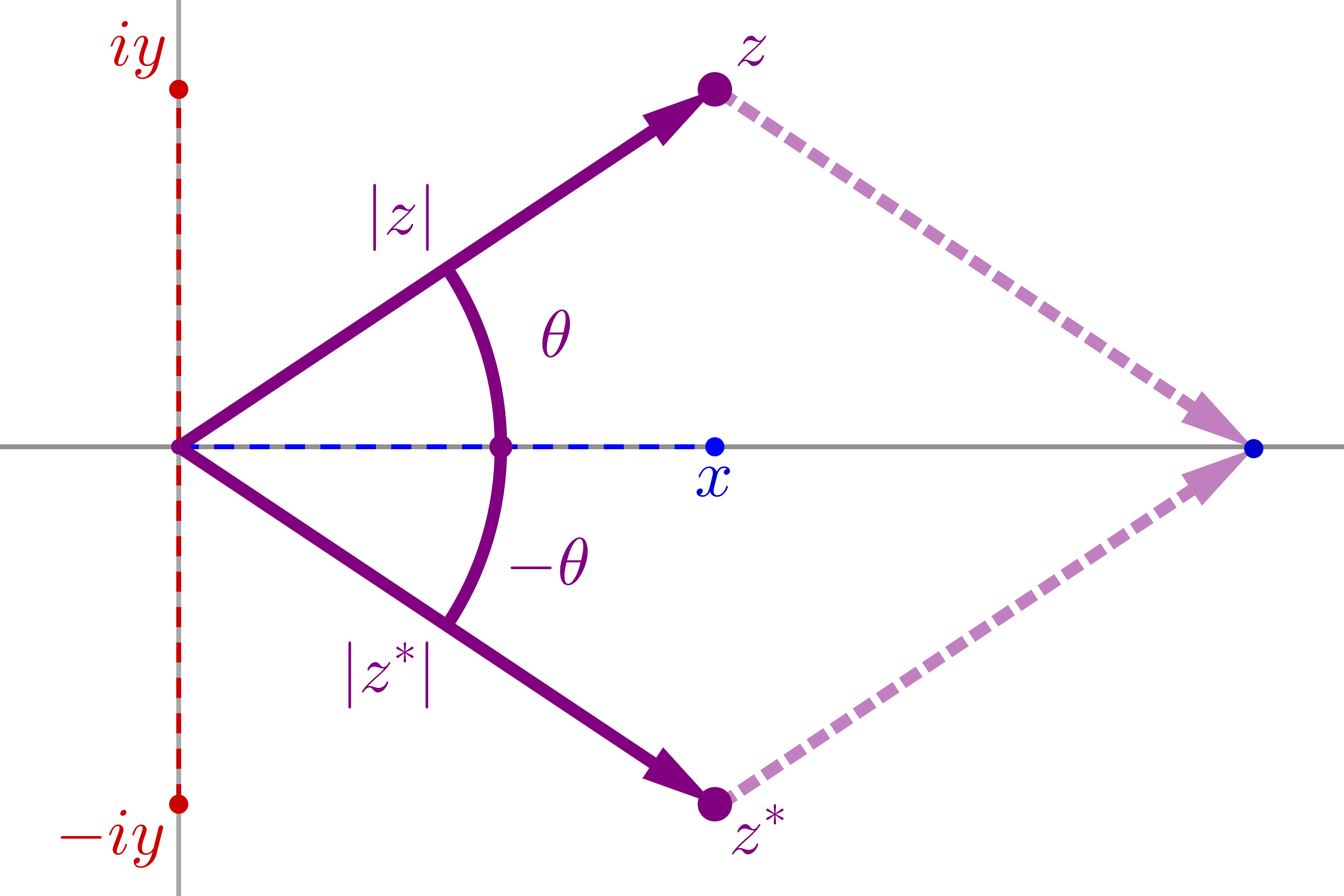
From the definition of sines, cosines, and tangents (see Section 1.3.3), we can use the geometrical right angle between the real and imaginary axes to define the angle of the the complex number, or the so-called argument of a complex number, denoted by . As is shown in Fig. 2.1, is the angular elevation of the complex number above the -axis. Since we know that while the real parts are identical, we know that . Using these angles we can then determine
| (2.22) | ||||
| (2.23) |
By solving the second equalities for and and then substituting these quantities in , we find
| (2.24) |
Note that this picture is consistent with just substituting in for to obtain a conjugate, because
| (2.25) |
where we have used the result of Problem 2.3 to set , and then we used the even and odd symmetry of the sinusoids: and .
Equation 2.24 shows that any complex number can be represented as the product of a radial part, and an angular part, as shown below
| (2.26) |
as a complement to the real-and-imaginary-part representations. Again, for the sake of completeness, the radial part is the modulus of the complex number while the angular part is the argument of the complex number. Take note that while the radial part is a real number like and , the angular part is still complex!
Thus, we have written any complex number in either a real-and-imaginary representation and in a radial-and-angular representation. These terms, although straight-to-the-point, are fairly clunky, so instead we name them the Cartesian and Polar representations of a complex number, respectively. The “pole” in this case is the distance (magnitude/length) the complex number is from the origin. A much more useful (and elegant) way to write a complex number and its conjugate in the polar representation is actually with an imaginary exponential , given as
| (2.27) | ||||
| (2.28) |
where
| (2.29) | ||||
| (2.30) |
Of course, to write such a thing, it would have to be true that
| (2.31) |
where is the base of the natural logarithm. Surprisingly, this result is true for all values of ! Remarkably, this result is not too difficult to prove even though it took a supergenius like Leonhard Euler44 4 Pronounced oiler, unlike how they said it in The Imitation Game, much to my chagrin… to first do it55 5 Hence, it is usually called the Euler identity. — it can be done with an introductory understanding of Taylor Series in a Calculus II course — although it is a bit beyond the scope of this chapter66 6 Don’t worry! We will come back to it later on and YOU will prove it in Problem 3.4.2 (I help you along though)..
Using the polar representation, it is possible for us to construct two of the most widely used expressions in all of physics — we are going to rewrite sine and cosine in terms of exponentials. To start consider the complex number of unit magnitude given by Eq. 2.31. Then it must be true
| (2.32) | |||
| (2.33) |
But by Eq. 2.10 and Eq. 2.11, we can write the real and imaginary parts of any complex number as a superposition of it and its complex conjugate. Then,
| (2.34) | ||||
| (2.35) |
Part of the reason why these relationships are so useful, is it allows us to treat trigonometric functions — objects that are defined geometrically — as exponential functions instead, which then allow us to employ a slew of useful (and quick) multiplication, differentiation, and integration rules to otherwise algebraically cumbersome functions. In physics, this polar representation of trigonometric functions helps us describe certain geometries and spaces in terms of essentially successive multiplications. As you can see in the chapter on Fourier Analysis, being able to convert sines and cosines into combinations of exponential functions makes otherwise impossible algebra much simpler. As we continue through this book, I will highlight more locations where these can be immediately implemented to make your life easier because the sooner you begin to feel comfortable with Eqs. 2.34 and 2.35, the faster you will begin to see through the mathematics of difficult subjects like signals, optics, and quantum mechanics to understand the underlying phenomena in a much more precise way. There is something potentially unsettling by writing geometric formulas as exponential formulas; it seems to imply there is a clear rotational aspect of multiplying two numbers, rather than the simpler stretching-and-shrinking interpretation that was valid with the real numbers. We study this more in the next section.
2.5 Multiplication = Dilation + Rotation
Let’s consider two complex numbers in polar representation, given by and . We will calculate their product and difference in the polar representation.
| (2.36) | ||||
| (2.37) |
Thus, by Eq. 2.36, multiplying a complex number by another is equivalent to dilating the magnitude of the first by the second and rotating the first complex number counter-clockwise by the second’s argument. Figure 2.2 shows the geometry behind multiplication. Likewise, since division is the multiplicative inverse, we should not be surprised by Eq. 2.37 which says that dividing a complex number by another is equivalent to constricting77 7 My word choice for “anti-dilating.” the magnitude of the first by the second and rotating the first complex number clockwise by the second’s argument.

What is often the case, at least in physics, when we deal with complex numbers, we are usually only taking about ones with unit magnitude — that is, the complex modulus is equal to one. Any complex number of the form in Eq. 2.31 fits this description. The reason why these numbers are so important is that they do not dilate the modulus of any complex number they are multiplying. Instead, they exclusively rotate the complex number they are multiplying. Figure 2.3 serves to help you get some intuition to how the multiplication = rotation bit works with more concrete numerical examples like and . Very often, physicists will talk of the phase of some quantity (such as in electromagnetic theory, optics, or quantum mechanics), and refer to the entire complex number as this phase. To be perfectly precise, the actual angle (argument) is the phase, NOT the entire complex number. However, as we have seen by Eq. 2.36 where , multiplying by the entire number only changes the total phase of the product, since it rotates the original number by . Thus, in terms of things we can experimentally detect (and therefore know are truly there), we can only find the resultant change of phase due to the multiplication of a complex number by another of unit magnitude.

Our ability to detect these so-called phase differences is actually rather remarkable. For example, in both classical and quantum mechanics, magnetic fields exert a torque on any charged object with angular momentum. This torque causes the charged object to precess in a circle; in other words, the charged object will behave similarly to how a toy top begins to wobble in circles around its central axis before it falls over due to gravity. In this case, the field that generates the wobble is the magnetic field instead of the gravitational field. Anyway, in quantum mechanics, a typical experiment to measure the phase difference goes something like this: generate a beam of identical particles, split the beam into two parts, do something to one beam and leave the other alone, then recombine the beams and see if anything happens. So one such experiment deals with measuring the intensity of particles with inherent angular momentum (spin) after splitting up the beam and having one part travel through a magnetic field over some distance. The amount those particles wobble due to the magnetic field then acts as the phase difference between the particles in the beam. As you will eventually learn, the intensity of the recombined beam is a function of the phase difference, meaning we can experimentally vary either the strength of the magnetic field or increase the distance the beam travels through it, and then change the intensity of the resulting beam of particles! For an example of such an experiment, check out [19].
Before proceeding, let’s take note of one special case of multiplication: exponentiation. In other words, we can raise any real number to the power by successively multiplying by itself times. For example, if and , then . Likewise, if we have a negative exponent, then we divide successively, while if has a noninteger fractional part, we take the appropriate root . Using the polar representation of a complex number , we can generalize exponentiation rather straightforwardly as
| (2.38) |
By setting a new angle , and a new radial part as , we have
| (2.39) |
Making use of Euler’s Identity (Eq. 2.31), we see that
| (2.40) |
Since the quantity can be written in terms of a radial and angular part, it must be complex-valued, as those parts yield real and imaginary parts. Thus which means our rules for complex numbers lead to closure under exponentiation! In other words, we cannot ever possibly end up with a non-complex-valued quantity purely by exponentiation88 8 This is a very good thing, mind you, for it essentially gives us motivation for starting to see if more complicated algebraic and transcendental functions always return complex numbers..
There is, meanwhile, a much more subtle identity that we may not have initially noticed while showing . We made use of a statement known as De Moivre’s Theorem that says for any integer
| (2.41) |
Looking closely at Eq. 2.41, we see that this statement is actually incredibly complicated. It manages to relate something as easy to compute as raising a number to an integer power to the much more difficult trigonometric functions, cosine and sine. But more importantly De Moivre’s Theorem puts the exponent inside of the argument of the trig function! Usually, there is no clear way to translate the argument of a trig function to anything outside of the function — for example for every value of . Trigonometric functions just don’t behave nicely like this. However, by making use of the complex plane, De Moivre’s Theorem gives us a way of applying algebraically simply operations to compute otherwise very difficult, if not outright impossible, quantities.
I do want to emphasize that De Moivre’s Theorem only applies for integer exponents, whereas Eq. 2.40 applies for all possible values of (even complex ones!). What gives? Where is there a difference? We look into this question next.
2.5.1 Roots of Unity
Let’s consider the case in De Moivre’s Theorem where . In this particular case, then if De Moivre’s Theorem were to hold, then it would be true (but it is not)
Let’s choose the easier case of and since on the left-hand side, we will have
This follows since and . There is no problem yet. The issue arises when we look at the right-hand side to find
(Remember that .) So, if De Moivre’s Theorem were to be trusted, we would find that . In other words, we would find that our answer implies that and this contradicts our rules for real numbers.
This result is not too surprising from an Algebra II point-of-view since we already know that both and , which we normally write instead as . But this means that the square-root function is mutli-valued, and in general the -root is also multi-valued. The problem with De Moivre’s Theorem is that it does not explicitly account for this phenomenon. We could easily generalize it to account for the multi-valuedness in exponentiation by rational exponents.
We start with the so-called Roots of Unity as they are both fundamental and something that we have already developed the motivation for. Let’s start off easy, and find the cubic roots of unity. We will proceed in the same way as we did before with the square-roots of unity. Here we have
Like before, we choose and because . There is actually another case we can consider, too: . Calculating each of these cases, we have
And so the cubic-roots of unity we found are
Hopefully, you aren’t satisfied with this derivation of the cubic-roots of unity so far because I just arbitrarily decided to include the part when I didn’t include it for the square-roots. The reason why I was able to include for the cubic-roots and not for the square-roots is because of the oscillatory behavior of sines and cosines — they repeat themselves every radians. So essentially, when looking for values that would show the roots of unity are indeed multi-valued, I needed to watch out for two criteria. First, I needed to make sure since we are taking about roots of unity, AND I needed to make sure that the right-hand side did not repeat itself. Let’s analyze each criterion independently, and by doing so, we will generalize the square and cubic cases to the -root.
If we want , then we need . But the value is totally real, hence the sine coefficient attached to the must vanish for our values. This condition holds for . Next, we are dealing with roots of unity, not roots of negative-unity. Thus, we can only allow for even multiplies of so that , where . So this explains why I kept choosing and then . But why not the negatives, too? The answer to that comes again from the even symmetry of the cosine function:
In other words, the cosine functions ignore the overall negative sign inside of their argument and produce the same result either way. Hence, we could include the negative values, et cetera, but we would ultimately always recover the same set of possible values.
Now we move onto the second criterion which says that cannot make the right-hand side repeat itself. We use the first criterion that we had established where all of the roots of unity will have values that are an even multiple of . Let’s call this multiple and write as
If we start with , then we will always find , as we expect, since . Then, as we continue to check through all of the possible multiples we have, we find the first repeating value at :
But this returns the exact same value as . Furthermore, any multiple of will ALWAYS be the same as the case. Meanwhile, all of the possible multiples up to are totally allowed because, in general,
the only case where equality holds is when . Thus, our -roots of unity are given as
| (2.42) |
in the Cartesian representation. In the polar representation, we pack the sinusoids into the exponential function to find
| (2.43) |
(Note that for all . I used the exp representation because the equation would have looked gross if I used e instead.)

The -roots of unity are quite nice geometrically because they chop up the unit circle ( radians) into regular -gons by dividing the full radians into equally-spaced intervals. A few of these are shown in Fig. 2.4. What is more beautiful from a physical point-of-view is that since the roots of unity form regular -gons inscribed within a unit circle, their sum must vanish. This can be directly applied to study cylindrically (and polygonally) symmetrical systems in physics; for example, point like-charges (masses) arranged in some polygonal shape whose net electric (gravitational) fields must vanish at their geometrical center. In more computational applications in physics, this property allows us to compute discrete Fourier Transforms of signals which is a mathematical operation that allows us to understand the signal in terms of its frequency-dependence instead of its time-dependence99 9 The Fourier Analysis chapter in this book does not deal with the discrete transform, but the tools developed in the chapter in the continuum can help you understand the intuition behind the discrete version..
To show how the roots sum to zero explicitly, recall the square-roots of unity: and . Together they form a line (lame), but their sum is . We can also do the cubic-roots of unity that form an equilateral triangle (less lame):
Now let’s generalize (disclaimer: this will be one of the more abstract things so far).
Consider the sum of the -roots of unity in polar representation, written as , and given as
If we look closely at the summation, we will see that we actually have a finite geometric series, defined generally as
| (2.44) |
for some value . In this case, and
To determine what this finite sum is, we can employ a few mathemagical1010 10 Bad pun? tricks that I highly recommend you work out with me. Knowing how they work WILL come in handy later on in your physics career, at least when it comes to handling finite sums. If you work these tricks out with me, then you are prone to remembering them in the future. Here we go.
We will calculate the quantity using the definition of given in Eq. 2.44, and at the end we will substitute in .
In the last equality, I used the definition of the finite geometric series again, except since the sum only goes to , then that means the proper subscript on is since . In this form, we cannot proceed because we needed , NOT . Thus we need to figure out a way to relate the two different finite sums.
Let’s consider now . If we look again at Eq. 2.44, we will see that if we were to add to , we would have
Hence, . Now we are going to substitute this expression in for inside the last equality for and isolate .
By moving the on the left-hand side to the right-hand side we have
and finally we have
| (2.45) |
which is the exact way to calculate a finite geometric series for any value of (the formula blows up at because if were 1 then we would have a step in our derivation, thus we had to implicitly assume that ). Finally, we substitute in :
| (2.46) |
And so it is true that the sum of all of the -roots of unity will always be identically zero! Furthermore, since a geometric series is built from multiplying the same object by itself a bunch of time, and we know that multiplication by a complex number of unit magnitude is a pure rotation, then the complex number represents a symmetry present in the set of the -roots of unity. The symmetry here is that our set of complex numbers are invariant under a rotation of radians — i.e. the number of points looks identical if we rotate all of them by the same angle! For example, if we have the square-roots and we rotate each number through the complex plane by radians, we have
as shown in Since the rotation maps the set of square-roots onto themselves, this rotation is the symmetry I was talking about that is directly embedded within the set of square-roots of unity.

Since the ambiguity in De Moivre’s Theorem is taken care of, we can return to Eq. 2.40 to account for all of the different possible roots of . Specifically, we can talk about any root , we have
| (2.47) |
Then, by extension, a complex number to any rational power (for example 4/3) can be written as
| (2.48) |
The power with raising a complex number to a rational exponent is that we can then use this as a basis for raising a complex number to an irrational exponent since we can always successively approximate an irrational number with a rational number. For example, . But how about raising a complex number to a complex exponent? We will study this and more in the next section.
2.6 Functions of a Complex Variable
In this section, we will study a few algebraic and transcendental functions of a complex variable. Unfortunately, we will not have time to study these functions beyond just domain and range, but rest assured that understanding the inputs and outputs of complex functions is totally sufficient for a B.S. in physics. As one studies either more math or more physics, ideas from Complex Analysis become relevant if not actually crucial, whether they be in the form of circuit analysis, fluid mechanics, or quantum field theory. I have some references for anyone interested at this point in their studies [20, 21, 22] (feel free to come back at a later date for them though!).
I have used the term “map” before when talking about functions, and perhaps you’ve heard others use that word in the same context. In more colloquial settings, people use maps to get from one place to another, and in this section the connection between a function and an everyday map will become clearer. We will see that functions, particularly complex-valued functions, serve to get from one place in the complex plane to another. To illustrate this idea, let’s consider the following example where we see how regions of the complex plane are connected through the function, or mapping, .
From Example 2.6, we can conclude a couple of things. First, complex-valued functions unite different regions of the complex plane. And second, specifically for this quadratic function, we chose to only consider the unit square. We could have chosen a square of size 2, or , or a gazillion. Then would also increase in size by Eq. 2.49. I will leave it to you to pick particular points on the square of side length and plug it into Eq. 2.49 to see how large the region in the -plane becomes (hint: try the points and ). Since we can choose a square of any size, we can artificially stretch the region in the -plane to infinity as we increase the domain in the -plane. Notice though, that as long as our domain is only in the first quadrant in the -plane, we will only ever be in the first or second quadrants in the -plane. This region is sometimes referred to as the upper-half plane. As you may see after doing Problem 2.6, other regions will map to fill the lower-half plane, and by extension, we can stretch regions out as well to fill the entire lower-half plane. Hence, the function maps the entire complex plane into the entire complex plane! Actually, functions such as these are specifically named entire functions since they are defined1111 11 Technically, functions are entire only if they converge everywhere in the plane. However, convergence is beyond the scope of this chapter, so understanding entire functions as simply being defined everywhere is good enough for right now. everywhere in the plane. Since we have begun to understand complex mappings in terms of complex domains and ranges, we seek to study a few more fairly commonly-used complex functions in physics.
2.6.1 Polynomials
For the first type of function, we consider functions of the form
| (2.50) |
where all of the constant coefficients are arbitrary complex numbers, but each exponent is a nonnegative integer. This class of functions, often denoted by the symbol for “polynomial of -order,” is the complex generalization of the real polynomials that you already know. This means that instead of only allowing ourselves to input real numbers into a polynomial, we now are allowing ourselves to insert a complex number as the argument of the function (in other words, an element from the domain). With this value of and by Eq. 2.40, we have
| (2.51) |
It is important to note that we are entirely allowed to compute every single one of these terms using the polar representations of the coefficients, if we had them given. Since each term is defined and computable, then we are definitely allowed to add all of their corresponding real and imaginary parts. Thus, for any that we throw at this thing, we will always be able to find its output as a complex number. Thus a general polynomial maps the complex plane onto1212 12 To be clear, there is a difference between the words into and onto. A function from set to set , , is said to be onto if every element of is in the range of . Pictorally, this means that there are no parts of that are not connected by to . Otherwise, mathematicians use the word into. the complex plane. Our conclusion is important because, just like with real numbers, complex polynomials are actually relatively easy functions to handle, whether it be in calculus, computational physics, mathematical modeling, et cetera, because we can handle them term-wise. Other functions, (like the transcendental functions) are not so nice.
2.6.2 Complex Exponentiation Revisted
The last time we dealt with complex exponentials was with deriving the rational generalization to De Moivre’s Theorem in Eq. 2.48. We were explicit, however, that the exponent itself had to be a rational number , where and are integers along the real axis. Now we have to ask the question of whether it is possible to raise a complex number to a constant complex exponent . In other words, we want to study the function .
Since , we choose to work with it in its Cartesian representation. Let and such that . Thus
Now, we will make the substitution of into the equation above.
Now, before proceeding further, since is a real number, that means it lies entirely along the real axis, and we can use our regular logarithms on it, since those are defined over the positive real axis. Thus, we choose to write , as the (real) functions and are inverse functions such that . When we make this substitution into , we can derive our final result.
| (2.52) |
It is important to note that the long string of symbols given in Eq. 2.52 is something that is entirely computable. What I mean by that is this expression is written in the polar representation of a complex number, where
Hence Eq. 2.52 is already in the form of a complex number, regardless of which values of and we choose! To be clear, if we were to convert back to a Cartesian representation then we would need to be careful with any ambiguities in the rational exponents, as is given in Eq. 2.48. But otherwise, we are free to map the complex plane onto1313 13 Since there are many possible roots for complex exponents, the -plane actually gets mapped onto the -plane in multi-valued ways, which we won’t go into. These peculiarities (translated to “headaches”in math-speak) are known as branch cuts, and special note really should be paid to them from a mathematical point-of-view. However, in physics, they are only noted if necessary. the complex plane via complex exponentiation.
2.6.3 Complex Logarithms
Since we have covered the case of exponentiation, it follows that we should cover inverse exponentiation, that is, we need to discuss how to find the logarithm of a complex number. To study this function, consider , where denotes “natural logarithm1414 14 In many advanced mathematics, the “common log”, denoted by , is used instead of . However, the “common log” of a number in physics is almost always given by . ”. Just as before, this problem is most easily tackled in the polar representation.
| (2.53) |
To be clear, in this derivation, we implicitly borrowed the logarithm of a product rule from the real numbers, , and we implicitly enforce that the natural logarithm is the function-inverse of . It is very important to note, however, that ANY complex number is invariant under a full rotation about the origin — therefore invariant under a rotation of , where is an integer. This is equivalent to saying . However, the exponents are additive, therefore
But if we apply this idea to , then we have . Thus, when we take a logarithm, we have
| (2.54) |
But wait. From Eq. 2.53, have
| (2.55) |
which seems to imply that if this equation is to be true. Since and are both nonzero quantities, this means that would have to be zero! However, we said can be any integer, not just zero. What gives? Did we accidentally stumble on a contradiction within complex algebra?
So the truth is that, with our current system of complex numbers, we actually did find a contradiction, and it has to do with our interpretation of multiplication as rotation and in the polar representation. But this contraction is not a totally new idea — it is similar to the idea that rational exponents are multivalued. It turns out that in the complex plane, the logarithm also accrues multiple values for the same input. In this sense, the full logarithm is not a function since for any input there are many outputs (so it does not pass the complex-version of the vertical line test). How do we deal with this problem? We use the idea of branch cuts to save the day, where a “branch cut” is a fancy name for specifying a particular range of the logarithm over a particular domain. In fact, this approach is identical to the one you learned in trigonometry, where we would only specify the inverse cosine () or inverse sine () on the interval , since there are (infinitely) many values of such that or . Although this is (sort of) passing-the-buck on the issue of having the logarithm be mutlivalued, it DOES allow us to retain our interpretation of multiplication as rotations in the complex plane — we just need to be careful about which branch we’re talking about when using the logarithm.
So the problem with the logarithm is due to the multiplicity, or rotational symmetry, surrounding the angle. Thus, it helps to define a principal branch of the logarithm, so there really isn’t a lot of ambiguity surrounding our equations. All we need to do is define the imaginary part of the logarithm over a -interval to keep things consistent, since it is the imaginary part in Eq. 2.53 that has the multiple values. The interval we choose may initially seem odd, but actually is more intuitive in physics, and is given by . Therefore, the principal logarithm is defined as
| (2.56) |
Here, the capital signifies the special branch of the multivalued logarithm given in Eq. 2.53. Notice though that there is a lowercase in the real part of Eq. 2.56. This is because is a positive real number, and we can always take a normal, non-multivalued logarithm of any positive real number. All of the multivaluedness, again, is only due to the imaginary part.
2.6.4 Hyperbolic Trigonometry
The final class of functions that I want to discuss is within the set of functions that most people refer to as hyperbolic trigonometry. The geometry is actually remarkably simple to jump to from normal, or circular, trigonometry. The latter is governed by the unit circle, defined by . We are instead going to be interested in the so-called unit hyperbola, defined by . Although the geometry may be interesting, I am going to be honest with you: the only time I’ve ever actually seen it be relevant is in orbital mechanics where trajectories matter, or general relativity, where the geometry of spacetime is the dynamical variable of interest (in other fields of physics, like Physics 1, the dynamical variables are position and velocity as a functions of time). With that said, the actual hyperbolic functions themselves are often incredibly useful tools to use in physics. They, for example, are used to describe how the electrostatic potential changes in space from a source. I have included Fig. 2.7 to help you see what unit hyperbola looks like, and how the hyperbolic trigonometric functions relate triangles to it.
The most commonly used hyperbolic functions are the hyperbolic cosine and the hyperbolic sine functions, defined by
| (2.57) | ||||
| (2.58) |
for any . Here the extra that’s attached is the hyperbolic part, and the notation is pronounced cah-sh while the part is often pronounced sin-ch. I’m not 100% sure why there is an added ch in the pronounciation, but my best guess is that sin-h is hard to say. Since I know that these real-valued functions will be brand new to most of you reading, I included a plot of them in Fig. 2.8 so you can visualize them. Notice that as , the hyperbolic sine and hyperbolic cosine become equal, whereas on the other side of the real axis, the and approach values equal magnitudes but opposite signs. Note that if we set and , then
which shows that these definitions of the and appropriately parameterize the unit hyperbola with the parameter . To better understand the parameterization, imagine as a unit of time, and and are the positions of a point moving along the unit hyperbola.
It is also really important to notice that the is an even function, whereas the is an odd function, in the sense that an even function has the property while odd functions have the property . I will prove these properties for the and to you below.
I wanted to point these properties out to you because they actually identically mimic those of the normal trigonometric functions, where the cosine is even and the sine is odd! There are actually a slew of other analogous properties between circular trigonometry and hyperbolic trigonometry, but I will not address them here. From here I am going to shift our attention to uniting circular trig with hyperbolic trig through the complex plane.
Okay, back to complex numbers. Consider the function . This time, we will choose to work with in its Cartesian representation so that . Then, using Eq. 2.57, we have
| (2.59) |
Thus, we have shown that the of a complex argument mixes circular and hyperbolic trigonometry. Furthermore, let’s assume that , meaning it is a purely imaginary (lateral) number. Then
| (2.60) |
This relationship goes the other way as well. If we consider then we have from Eq. 2.34
| (2.61) |
Since the imaginary arguments can be used to convert between circular and hyperbolic trig using these equations, we conclude that hyperbolic triangles are really just a lateral/adjacent form of straight-line versions. This conclusion could have actually been reached with the unit circle itself, , if we changed the part to an imaginary number , thus converting the unit circle to , the unit hyperbola! Perhaps if we had not given the name of “imaginary”, then we could have known more about geometry, in general, immediately from the start.
2.7 Concluding Remarks
In this chapter, the fundamentals of complex algebra were introduced and used to generalize a few commonly used real functions into the complex plane. Knowing how to use complex numbers to study physical systems is particularly helpful. For example, it is pretty common to treat all electromagnetic waves as traveling complex exponentials given by , where is the wavenumber of the wave, is the position of the wavefront, is the frequency of the wave, and is the time. To be clear, the electromagnetic waves are purely real objects meaning that all of their physical properties would be quantities that we would associate with the real line (they are not lateral quantities, whatever those may be…). So why are these imaginary/lateral parts relevant in physics? It turns out that exponentials have a plethora of useful properties in calculus and they are much more manageable than the trigonometric waves defined by sines and cosines. Thus, we usually only need to worry about the real part of the electric and magnetic fields. Meanwhile, whenever the waves move through a material, it turns out that the can be identified as having both a real part and a lateral part, where the latter actually plays a role in the heat-loss of the wave in that medium (this property is called attenuation). In other words, knowing how to split up complex numbers into real and imaginary (lateral) parts and more can tell us very important things about how physical objects interact with one another. And this case is one where we use complex numbers to make our mathematical modeling simpler — it does not include situations in physics where the whole complex plane is absolutely necessary, such as anything where the word “quantum” is involved.
There is still a lot of topics within the topic of complex numbers at large, but this chapter hopefully gives you a solid foundation in something that, once you get the hang of it, will truly make that math you use in physics much simpler, and by extension, your life much easier. Not to mention, complex algebra at least makes things like numbers a little prettier to look at.
I have included a table of helpful equations (Table 2.1) for you to reference for whenever you need them later on in your career. They also have a reference to the text where they were described.
| Equation Description | Equation Formula | Text Reference |
|---|---|---|
| Definition of Complex Numbers | Eq. 2.8 | |
| Definition of Complex Conjugate | Eq. 2.9 | |
| Real Part of a Complex Number | Eq. 2.10 | |
| Imaginary Part of a Complex Number | Eq. 2.11 | |
| Addition of Complex Numbers | Eq. 2.12 | |
| Product of Complex Numbers | Eq. 2.13 | |
| Quotient of Complex Numbers | Eq. 2.14 | |
| Modulus of a Complex Number | Eq. 2.16 | |
| Polar Representation | Eq. 2.27 | |
| Argument of a Complex Number | Eq. 2.30 | |
| Euler’s Identity | Eq. 2.31 | |
| Cosine Formula | Eq. 2.34 | |
| Sine Formula | Eq. 2.35 | |
| Multiplication as Dilation and Rotation | Eq. 2.36 | |
| De Moivre’ Theorem (for Integer ) | Eq. 2.41 | |
| Roots of Unity | Eq. 2.43 | |
| -Term Geometric Series | Eq. 2.45 | |
| Sum of Roots of Unity | Eq. 2.46 | |
| General Complex Exponentiation | Eq. 2.52 | |
| Principal Logarithm | Eq. 2.56 |
Chapter 3 Calculus of a Single Variable
Up until now, I have not assumed that you have any prior knowledge of calculus, mostly because it is frankly unnecessary to understand vectors and complex algebra. Thus, everything that we have covered is totally static. It, in no way, describes anything that can possibly change at all. For example, if the position vector of a particular object is known at a particular time, we would thus far only have the tools to describe the object’s vector at that time. Sure, we could resolve the vector into its components, we could talk about the direction of the vector, we could talk about it being orthogonal to other vectors, but we would have NO WAY of talking about how that vector is changing at that time. Hence could not speak of how the object will move in time.
You might be wondering why we could not just reference the object’s velocity vector at that time, since surely the velocity will tell us about how the position vector changes. As we will see, this is absolutely true. However, none of the mathematical tools we’ve discussed so far allow us to describe this change. Meanwhile, you can definitely intuit how position will change because you have experienced changes in your everyday life. Our goal in this chapter is to develop your natural intuition into something mathematically precise and immutable — our goal is to develop calculus.
As a heads up, chapter is going to be dense. Like, degenerate matter dense11 1 A classical model of the degeneracy will probably suffice though.. We are going to cover essentially the same amount of material that one would see as they progressed from a Calculus I and II sequence of courses. Although we will cover a lot of material, it will be condensed to a form that is sufficient for implementation in physics. Truth be told, once you understand derivatives and integrals from a geometric/changey perspective, then the number of dimensions rarely makes a difference to a physicist. Sure, it might add a few extra terms here and there, but the actual modeling of the natural world using rates of change is what matters to us, and it is almost always easy, if not trivial, to discuss the laws of physics using calculus. That is not to say that actually solving problems in physics is trivial, it isn’t, but the nontriviality of the problem solving in physics is partly due to the inclusion of our clunky form of algebra with calculus. The other part is usually just because nature is smarter than us.
I plan to introduce many calculus topics at are relevant for physics in ways that are easy to visualize. I am not going to get too bogged down in the details about which functions have which derivatives or antiderivatives, although I will talk about a few important ones. Calculus really should not be about the memorization of a bunch of special-case formulas; when it is, it is usually very hard for students to see its value or applicability. Thus, I will reference outside sources for specific formulas if they are not quick and easy to derive (tables of derivatives and integrals are ubiquitous and freely available on the Internet). Although the transition can be hard, once you are able to see beyond the mess of special cases, using calculus to describe the universe will be effortless, and you will probably wonder how you didn’t already describe it is such a fluent way22 2 Okay, so maybe this is a little anecdotal and waxing poetic, but, hey, if using calculus were worse than what we had before, why would we still be using it?.
3.1 Position, Velocity, and Acceleration
People usually have an almost instinctive understanding of how things move (with the exception of feathers and bowling balls in free fall). Unfortunately, it took an incredible amount of time for us to develop a means of communicating our understanding with others in a precise way. We can thank people like Galileo and Newton for figuring that last bit out for us. In historical hindsight though, developing the crucial ideas of calculus are pretty straightforward.
We are going to start by exploiting the position, velocity, and acceleration of some object (maybe a car or volleyball or bug) and we will be careful to remember that each is a vector. Furthermore, let us assume that we know the position vectors at a few different times, and let us denote these vectors by . Using vector addition (recall tip-to-tail), we can then define a vector that changes the position at one time to one at a later time . Here this represents an increment in time, for example, it could represent a year, a century, a second, a femtosecond, a unit of Planck time, et cetera. Physically, this increment in time would be whatever time difference it takes to get the object from one position to the next. This change vector at time is going to be denoted as and connects the position at , , to the position at , , as is shown in Fig. 3.1.

A question that follows from this set up would be something like, “Is it possible to describe how quickly the object moved from to ?” Intuitively, we might propose that the change in position, or the position increment, , is proportional to the increment in time, . For example, if we were running at a specific pace for a longer period of time, we will travel farther. However, time is scalar, whereas the change in position is definitely a vector by Fig. 3.1. Thus, we are left to define the velocity33 3 For anyone who already knows calculus, this is the average velocity. of the object at time as the vector responsible for the change in the object’s position. This is denoted as and can be written mathematically as
| (3.1) |
or if we divide both sides by the scalar time increment, we have
| (3.2) |
It is important to remember that at this point the things everywhere are meant to symbolize that the letter immediately before is a function of ; it does not mean multiply everything by . For example, means that the velocity is a function of time rather than multiply and the scalar .
By looking at Eq. 3.2, we see that the equation has the form of a slope, in that it is a function that has a change divided by a change, or more colloquially, it has a rise-over-run type form. Furthermore, we can see where the units of miles-per-hour or meters-per-second come from, since we multiply the position vector measured in units of length by the scalar which has units of per-time. Also, using this definition, since the time increment takes on the value of whatever time-recording device we have allows, if there is no change in position, we conclude that there is zero velocity. Likewise, if there is ever a time where the velocity is zero, then there will be no resulting change in position. Alright, now that the relationship between changes in position and velocity is established between two points in time, what happens when we introduce more points? Or from a more scientific perspective, what happens when we measure the position of an object at a greater number of points in time?

For simplicity, let’s assume we know the position of a particle at three points in time: , , and . Then, just as we did before in Fig. 3.1, it is possible for us to connect the position at with that at , and we can now connect the position at with that at . A picture of this scenario is shown in Fig. 3.2, and in this figure, it is evident that there are really two changes in position:
Thus, we may ask “what is the change in the change in position?” Let us denote this change of change in position as , since the change of change position occurs at . Let’s denote the change of change as , and evaluate it directly
If we now assume that this change is proportional to some vector rate, just like we did when we came up with the notion of velocity, and denote this rate as , then we can posit that
Here . Solving for directly, we have
In the second equality, I moved one of the s into the numerator to make two fractions because these fractions are defined explicitly in Eq. 3.2. Using this definition, we have
| (3.3) |
which we recognize as the definition of acceleration44 4 Average acceleration to be precise. Again, this equation is one that has the form of a slope. Further, we would say that if there is a change in velocity, then there must have been an acceleration to cause it. However, since the acceleration is related to the change of change in position, we could also say that a “second-order” change in position is due to the existence of an acceleration.
So what have we learned by measuring more points? Well, it appears that each time we measure a new point, we can define a new rate associated with the addition of a new position measurement. This is generally true for position measurements. Actually, the names for a few of the even higher order changes () are the jerk, snap, crackle, and pop [23]. We also know that the little time increment is some measurement, but its actual value depends on the time-measuring device we have (for example, atomic clocks have smaller s than grandfather clocks). In principle, we could have exactly one position measurement for every single time measurement we have, and let’s assume we have total of these position measurements. Then we could write them down in a table of sorts as
And so each time there is a change in position, we would presumably have a corresponding velocity measurement, and additionally, each time we have a change in velocity we would have an acceleration. So we would have two more rows in that table
Here, the dashed marks appear since there are no changes initially for either the position or velocity; thus there are no velocities or accelerations at this time. To better help visualize this table, imagine that all of these measurements came from an object’s trajectory as that shown in Fig. 3.3, where the object starts at an initial position of and moves to a final position of . In the figure, the blue points represent the positions as functions of time (remember that these are all vectors, hence the ghostly vectors to and ), the red dashed vectors represent the velocities as functions of time, and the green dotted vectors represent the accelerations as functions of time.

An important highlight from drawing out all of these position measurements is that the velocity vectors can really be seen to connect all of the position measurements together. More precisely, if we wanted to know the position of the object at any time measurement, let’s say at the time increment, then we could find it by starting at and then adding all of the changes in position up until the increment. In other terms,
All of the s here show up from the implicit definition of the velocity at a point. The equation above can be written much more succinctly with summation notation, and so we have
| (3.4) |
Although it is harder to visualize from Fig. 3.3 (but not impossible!), there is actually an analogous summation relationship that exists to relate the velocity at to all of the intermediate accelerations:
| (3.5) |
These equations have the form of the area of a rectangle, where is the width of the rectangle, and the velocity or acceleration would be the height of the rectangle. Furthermore, we actually add up all of the intermediate areas to find something new.
In short, this is all that calculus is: either evaluating slopes or adding up a bunch of boxes. If we want to describe how quickly something changes in terms of another variable — for example, if we want to find how fast position changes as a function of time — we would use a slope. If, on the other hand, we wanted to describe the aggregate effects of many successive actions — for example, if we want to find out where our final position is after moving with a bunch of different velocities — we would add boxes. Even further, we can undo the effect of taking a slope by adding a bunch of areas together; an operational inversion analogous to how multiplying something by and then dividing the result by returns the original something. And that is truly all of calculus. There really is nothing else to conceptualize.
However, like most things, this conceptualization is easier said than done. And that’s okay. As we progress through this chapter, we will study many more applications of these ideas and refine them into some theorems. Fortunately for us, the context of this chapter will largely be the natural world, and so if the mathematics ever gets too messy, we can always find real-world analogies to bolster our intuition and understand which message the math is trying to convey.
3.2 Continuity
We have discussed how slopes and box-addition represent function-transitions between position, velocity, and acceleration. But everything we did was built on the assumption that we were taking measurements of time with some device that only measured in increments of . While this picture is accurate from a numerical perspective, and definitely from an experimental point-of-view, it is not necessarily physical and certainly not mathematical.
Physically, objects have positions at intermediate values between the points we measure. We unfortunately are limited by how quickly we can measure something’s position; however, this is no way implies that objects only move in discrete ways. In principle, if we were able to “take more measurements” then we could describe an object’s position, velocity, or acceleration at any time that we wanted.
To better illustrate this idea, we assume that something only moves over a fixed time interval, perhaps and that we have made a total of measurements. Then the time increment would be
Notice that this time increment gets smaller when the number of samples gets larger. If this is not clear, choose to be your favorite number (physicists really like ) and then divide by successively larger numbers — for example, , , , …, , … So as long as the is a fixed number, will get very small as gets very large.
The small time increment is helpful, because it allows us to probe more time-values. For example, if , , and , then we can talk about times like
But we could never reach a time value like , since our time increment is larger than that extra . In other words, our resolution is not good enough to see a time increment of . So what can we do? Instead of only taking measurements, how about we take ? Then we could have
By the same argument, we could jump down to a resolution of 0.001 by taking 1000 measurements to have
Hence, it is clear that by increasing the number of samples, we can know the position over smaller time increments and therefore observe what happens at those intermittent steps that we would have been incapable of observing before. So now the question is: “how many samples do we need to get a time increment to probe time up to any arbitrary level of precision ?”
To solve this problem, we just need the time increment to be less than this arbitrary precision (before ). Thus, what we do is posit that , or
| (3.6) |
The second inequality55 5 This inequality rule can be tricky for a lot of people the first time they see it. Most people know that if you multiply an inequality by a negative sign, then you must flip the inequality. The same is true for division. For example, it is true that , but it is not true that , when we invert the inequality. is our answer. I recommend you test it for yourself.
The beautiful thing about this idea is that can literally be anything, as long as it’s positive. That means we could increase it or decrease it at will — this is the math equivalent of increasing or decreasing the volume of your phone66 6 Or whatever the cool sound-emitting technological marvel you future people use., except there is no upper or lower bound! Thus, we could, at least in principle, probe time measurements to any level of precision we want. All we would need to do is take enough measurements.
In mathematics, we give this idea the name, limit of a sequence. In this case, the sequence would be , and the elements of the sequence would be each with a incrementally higher value substituted in. In this case, we would say that the limit of would be zero since we can definitively get within a precision of of zero using the inequalities above. More formally, we would say that the limit of some sequence , denoted by , exists by the following criterion:
The sequence is said to converge to the limit if there exists positive integers and such that for every , whenever .
When the limit does in fact exist, we say that
| (3.7) |
where the calculation of how many measurements are required to reach a precision of is given by the positive integer and the “taking enough measurements” is taken into account when in Eq. 3.7.
Knowing more and more precise time measurements is great, but what does it get us? How can we be sure that there will truly be a position measurement for us to take if we zoom in on the temporal axis with smaller and smaller time increments? To the best of my knowledge, in physics, we assume that this is always true for moving objects. But this would imply that as we more and more precise time measurements, we could get more and more precise position measurements. Or at least, if the position at one point in time is known, then the position as should be nearby that at . Otherwise, the object would somehow jump/teleport to another location randomly. And that would be weird/not anything we have ever observed, so in physics we assume that we can always zoom in infinitely far for all spatial and temporal variables ().
But how would we represent this mathematically? For this case, we will assume that we have taken infinitely many temporal measurements so that we can zoom in arbitrarily around some special point in time, let’s call it . If we have zoomed in to some arbitrary level of precision, now denoted by 77 7 The lowercase delta is because our precision is tiny, so I figured a little variable would be appropriate., then we can probe any time values within what’s called an open ball of radius . The ball itself is defined as the set of all -values that are within the radius of the central point , and for those who are interested it is written as
In a single dimension though, this ball is just the open interval along the real line. It is a circular disk in two dimensions, and actually is a ball (sphere) in three dimensions. In four and higher dimensions, it is harder to visualize88 8 Yes, this is a dare to prove me wrong..
Anyway, we want to be sure that an object doesn’t suddenly teleport elsewhere, so we need the position of an object at time to be nearby the position at time . Therefore, if we can find a position ball whose radius is somehow the result of the precision we chose, then we can guarantee that the position of the object at time will always be within the vicinity of the position at time . And most importantly, means
| (3.8) |
where is a finite number, of again, arbitrary precision.
This whole idea that zooming in far on the independent variable consequently leads to us freely zooming on the dependent variable is what is known as continuity. To be more mathematically precise:
A function is said to be continuous at if there exists a for every such that for every where then implies .
When the above statement holds, we call the output the limit of as which is written as
| (3.9) |
Sometimes, the limit is instead defined as so we can study functions where need not be defined.
The definition above is what you may have seen/heard of before — it is the - definition of continuity — but it is strictly in one-dimension, whereas actually everything else up until this point was in an arbitrarily high number of spatial dimensions; so maybe we were taking about an object only moving along a single axis (one-dimensional), or on a curve on a surface (two-dimensional), or even in a trajectory through space (three-dimensional). Here we condensed back to one-dimension with the - definition of continuity, because the mathematical precision in higher dimensions is actually a little too nuanced to jump in with immediately. Actually, to be completely honest, I don’t think the definition, as it is written above, has ever come up in a physics class that I’ve taken. However, the idea of being able to zoom in as far as we like does come up constantly; that is why I spent so much time developing the intuition behind the - definition of continuity. Nevertheless, I do want to unpack that definition a little, because it will be extremely relevant for things like derivatives later on.
First things first, the statement translates to “function that has real number inputs (first ) and then outputs real numbers (second ).” This means we are only dealing with the good-ol’ one-dimensional functions that you learned in high school. The next thing that is listed is that this definition of continuity only applies for functions at a single point in the domain. It says nothing about the continuity of at nearby points. The actual requirement for continuity is that there has to be an , a.k.a. an arbitrarily small number, to zoom in on nearby when we zoom in on itself to a chosen precision of . Therefore, this definition posits that the existence of the precision guarantees the existence of the precision in the independent variable. This means that continuity allows us to continue taking smaller and smaller independent-variable increments to measure smaller and smaller dependent-variable increments, just like our intuition with an object’s position informed us. So this definition, although I agree that it is pretty intangible the first time you see it, incorporates all of what we’ve discussed in the section so far, but it does it in a much more concise manner.
Example 3.2 shows how we might use the definition of continuity to show simple functions are continuous. The truth is that it usually takes a different algebra tricks to establish the continuity of individual functions, and oftentimes these tricks are NOT obvious. If you ever take a course in mathematical analysis, you will see it. Therefore, it usually helps to establish the continuity of general classes of functions, like that of sums, products, or compositions, because we can then argue that whatever messy function we have is truly just a combination of continuous functions. Thus, I am going to prove a few theorems to you regarding the continuity of sums, products, and compositions.
Disclaimer: the proofs will be pretty abstract, and so if it is too hard to follow at first, that’s okay. The fundamentally important continuity rules in physics will be the numbered limit equations that follow each proof, but I wouldn’t be able to live with myself if I just told you what they were without justification. I mean, this is supposed to be science after all, right?
Before we proceed to this point, we need one very important theorem concerning the absolute function: the so-called triangle inequality. It states simply that for any , we have
| (3.10) |
A proof of this statement is straightforward, and follows from the fact that for all real numbers. It goes as something like this,
Thus, . By taking the square root of both sides, we have the triangle inequality; a theorem that gets its name because it essentially says that if a triangle is made up of three sides, one side cannot have a magnitude greater than the sum of the other two. This inequality will help us establish that sums of continuous functions are continuous.
Now for continuity in summation. To prove this, consider the function , where and are both continuous at . Since both and are continuous at , then there must exist -precisions for both functions for every -precision, namely and , respectively, such that
Then, by substitution into , we have
Thus, when we define , where the function outputs the smaller value of and , then we have that implies for every . This means that when and are continuous at , so is the sum of the two. I want to emphasize that this conclusion implies the following limit rule:
| (3.11) |
Hence, the limit of the sum is the sum of the limits. Furthermore, if (and only if) both and are continuous over all of the real numbers, then so is their sum .
We next want to prove that the product of two functions that are continuous at is also continuous at that point when two functions are defined99 9 The defined condition guarantees that I can write something like and not have is accidentally blow up to infinity. at . Now let , and let the definitions of and be modified a little from what is given above as
These odd looking definitions will come in handy later on so that we will find and not some function of . Then we have by substitution,
Before continuing, we must figure out a way to deal with the because we do not know the specific value of at — we only know that is defined and that is continuous at . But since is continuous at , we are free to zoom in as far as we like on and we are guaranteed to be able to find an -interval that corresponds to our -precision. Thus, what we will do is choose to limit our -precision to be less than a set number, for example, . Then, by the continuity of , there exists a such that
Then we can say using the triangle inequality that
where the last inequality holds for every such that . Okay, so now that we have these conditions in place, and if we remember that , we can define our -precision such that . Then for every such that , we have
Since we were able to find an for every such that implies/leads to , then we can conclude that is continuous at . This time, the corresponding limit equation would look like
| (3.12) |
or the limit of a product is the product of limits. Just as was the case for the the sum of continuous functions, if both and are continuous over all of the reals, so is their product. However, if only one function is continuous everywhere, then the product is NOT continuous everywhere — it, too, is limited1010 10 Nice pun, right? to only be continuous for the values where both of its factors are.
The last continuity rule deals with compositions of functions. As a brief review compositions are sometimes written as or . They are functions that look something like this: if and , then . Thus, the notation of really just means put whatever the output of is into as the input. Although this class of functions may seem like more of a special case compared to sums or products (it did to me the first time I learned of it), compositions of functions appear everywhere in both calculus and physics. Thus, knowing how they behave is imperative.
Our goal in particular is to show that compositions of continuous functions are also continuous. To do this, we then need to show that a function is continuous at the point , given that is continuous at and is continuous at . To make this proof a little clearer, define
By the continuity of at , we know that for every , there exists a such that
Then by the continuity of at , we know that for every -precision, there exists a such that
Therefore, since we want something that looks like
then we choose such that our final statement reads as
for every . As long as both and are continuous everywhere, then the composite function will be continuous everywhere. If there are any points where is not continuous, then the composite function will not be continuous at those points1111 11 There is a huge caveat here: sometimes functions that are not specifically defined at a point can still look continuous at that point. These types of function discontinuities are called removable discontinuities or holes.. The corresponding limit equation for this composition property can be written as
| (3.13) |
which can be summarized as: the limit of the composition is the composition of the limits.
Again, these continuity rules (Eqs. 3.11, 3.12, and 3.13) are incredibly useful tools to determine if any function is continuous, or at least continuous at a specified point.
Although the ability to potentially take an infinite amount of measurements is great, it is honestly more helpful to know, for example, how an object is moving because we can then predict where it will be in the next instant in time. In physics, equations like these are called equations of motion, and the pursuit of these equations is pretty much all that physicists want to find for they all us to predict the future. Anyway, in order to be able to actually obtain the position of an object at every position, we need to know the velocity exactly at every time. So that means our increment would have to go to zero in Eq. 3.2! Furthermore, if we were to predict the object’s position, then the number of terms we would have to add in Eq. 3.4 would go to infinity! In summary, the goal of calculus is to obtain finite numbers when either dividing by zero or adding an infinite number of terms together. The amazing part is that this ability stems directly from the idea of continuity.
3.3 Differentiability and Integrability
Without further ado, I’ve been building up the idea that there are two major fields in calculus: one that deals with ratios (slopes) and one that deals adding terms together (areas). When we refer to the study of the slopes or areas of functions as differentiation and integration, respectively, and we give the exact slope the name of “derivative” while we call the exact area “integral”.
It is very common for math courses to present the derivative an integral as two separate objects and then combine them later on. I will instead try to introduce them as simultaneously as possible so that they are inextricably paired in your mind just as addition and subtraction or multiplication and division are. We will then jump back to higher dimensions because our job as scientists is to explain the world, and the world is not just one-dimensional1212 12 Some people think it is 11-dimensional., and so we will have to deal with the higher dimensions almost immediately to explain the phenomena we observe. The nice thing is that the ideas of calculus generalize quite easily — some of the applications of calculus do not generalize nicely, but those harder applications are largely the topics of other courses and are outside the scope of this book. Again, I will not list a bunch of specific derivatives or integrals because they are all over the place on the internet or in other books. Our goal is to get a better understanding of how they work and then if you need the specific formulas outside of this book, you can use them fluidly as they arise.
3.3.1 Definition of Derivative: Rise Over Run
We start with derivatives. What we do here follows from what we have built so far when we combine the idea of rates and continuity. We seek an object’s velocity at every single instant in time, and the only way to do this experimentally is to take infinitely many time measurements so our time increment () is small enough for us to connect any instant in time with another instant. Here, when we say “instant”, we mean a literal point along the temporal axis with absolutely no uncertainty. So experimental measurements are out of the question because it is impossible for anyone to measure something an infinite amount of times, but luckily, the continuity framework we developed allows us to look at the overall behavior of the slopes of functions as our time increment gets infinitely small, and if the slopes seem to converge to some finite value, then we extract this value as the instantaneous slope, or the derivative of our function.
We start by defining the derivative of a function at a specified point as the following
| (3.14) |
The notation here of the big vertical line with the subscript of translates to “evaluated at the value of .” Notice then, that the function must be continuous at for the limit definition above to actually be defined. We say then that if this limit can be computed, that is to say if the difference quotient,
| (3.15) |
is continuous at , then the function is differentiable at . Here, if we define the change in the input variable as , and we define the associated change in the dependent variable as , then the equation above becomes
| (3.16) |
and so it is a little clearer that the derivative truly is an instantaneous slope of , as the fraction inside the limit is just the rise-over-run formula that you learned in algebra as the slope of a line. In this formula, I have omitted the vertical line telling us where to evaluate the derivative just to make it a little aesthete. Make sure you remember that the derivative is evaluated at a point though, and if a formula in general does not include the vertical line, it is implying that the equation for the derivative holds FOR ALL inputs.
A lot of non-pure-math people take Eq. 3.16 as justification of saying something along the lines of “the derivative is when we take the limit as .” This is only true in the most literal interpretation possible, because, as you may have noticed, the s in the left-hand side of Eq. 3.14 and Eq. 3.16 just appeared as soon as I defined the derivative; thus their appearance is purely a notation, and not any physically or mathematically meaningful. With that said, the reason why this -notation is helpful is because it does remind us that a derivative is a slope, but its calculation comes from a limiting process; that is, we must study the continuity of the function at to evaluate its derivative at that point.
For the sake of completeness, before I move on to showing you how to calculate a couple of simple derivatives, I need to let you know that, unfortunately, there are about as many notations for derivatives as there are baryonic particles in the universe. Okay, that’s not true. But there are a bunch of different notations that people use, and the context kind of drives which one is used where. My personal favorite is the fraction of the s, known as Leibniz’s notation, because of its aforementioned relation to slopes. But some other ones that you might see are boxed below.
And there are a few more nightmares that come about for slopes of slopes (think acceleration) that you can find here [24]. I will almost exclusively use the Leibniz notation throughout this book, but for your own future reference, it is always a very good idea to make sure you understand the context; for example, I and many other physics books use to denote a different value than , but math courses almost always use the to denote a derivative.
Example 3.3.1 shows how one would use the limit definition to find the derivative of a constant function, a simple linear function, a parabola, and a hyperbola. What is conventional at this point in many calculus references is to just list out a bunch of other derivatives because there are a bunch more that can be computed. A simple Google search would return any such list, but I’ve included a couple here for your reference [25, 26]. Then, in practice, one would just use the functional expression (like Eqs. 3.18, 3.20, 3.22, and 3.24) whenever one is needed. It is truly a rare thing in physics for one to use the limit definition to ever compute a derivative1313 13 However, the limit definition is used constantly in fields of computational physics to evaluate the numerical derivative — in essence, one chooses a point in the computer and then finds a number with the difference quotient (Eq. 3.15)., although we do use the limit definition often to say there exists a derivative within our equations. Nevertheless, there are three rules that we must establish with the limit definition before we can move on. These are the linearity of differentiation, the product rule, and the chain rule.
Linearity of the Derivative
An extremely useful and important property of derivatives is that they are linear operators. Recall from Eq. 1.39 that a linear operator has the following property:
| (3.25) |
where we have replaced the vectors in Eq. 1.39 with the functions and . Thus, our mission here is to prove that the following statement holds
In other words, we seek to prove two things: first, derivatives ignore constant coefficients, and two, the derivative of the sum is the sum of the derivatives.
Okay so now we start with the following function: , where . Let’s assume that is differentiable at the point . Then we have
But is a constant function which is continuous everywhere and converges to , and by assumption the difference quotient for is continuous at and converges to the derivative of , therefore we can use the limit of the product is the limit of the product rule in Eq. 3.12. Thus,
| (3.26) |
And so we find that, as long as is differentiable at any arbitrary input , then
| (3.27) |
that is, the derivative operator indeed totally ignores any constant coefficients.
Now we must talk about sums of functions. So suppose we have a function , where both and are differentiable at . Then, we simply have
By assumption, both difference quotients are continuous at and converge to the derivatives of and at , therefore we can use the limit of the sum rule in Eq. 3.11. Thus,
| (3.28) |
As long as and are continuous at any arbitrary input , then we can write
| (3.29) |
Therefore, we do see that the derivative of the sum is the sum of the derivatives.
Finally, we combine these two proofs together into our statement of linearity. Take the function , where and are at least differentiable at . Then,
When we combine the first and the last equality, we indeed have our statement of the linearity of the derivative, given explicitly as
| (3.30) |
and again, whenever both and are differentiable everywhere, so is their sum. In this case, the equation above would shed its vertical lines as
| (3.31) |
as we had as our claim.
The Product Rule
Now that we have established the way in which derivatives behave with sums (Eq. 3.29), how about the derivative of a product? This proof will take a little more work, but combining it with sums will allow us to calculate many individual derivatives whenever they arise. So without further ado, consider the function where and are both differentiable at . Now we want to determine what the derivative of is at that same point.
Since both and are differentiable at , they are both defined and continuous at . Additionally, their difference quotients are also continuous at . Therefore each term in the limit is continuous at and so we can use Eq. 3.11 to split up the sum, and then we can use Eq. 3.12 to split up each of the factors in each term. Thus, we have
When we are free to omit the vertical lines, then the equation above has the more common form of
| (3.32) |
which is known as the product rule for differentiation. It essentially says that the derivative of the product is more complicated than simply the product of the derivatives. However, nice little mnemonic phrases exist for the product rule, such as “the derivative of the product is the derivative of the first times the second plus the first times the derivative of the second.” Okay, so maybe the mnemonic isn’t that great. But the formula itself is not that difficult to remember, so that’s good, right?
The Chain Rule
The final rule that needs to be covered is what happens when we have a composition of functions, as was our last case for continuity. Again, compositions of functions arise all the time in physics and math, so we better know how to handle them when they do. So suppose we have a function , where is differentiable at and is differentiable at . Now we employ the limit definition of differentiation to study the tiny variations in associated with the variations in nearby .
The above equation might look a little gross because of all the parentheticals. Therefore, let’s define and , where is continuous at , as we assumed was. Then we have a limit of continuous difference quotients, and so we can split up the product according to Eq. 3.12.
When and are differentiable everywhere, then the formula above becomes what is more widely recognized as the Chain Rule for Differentiation, given by
| (3.34) |
The formula above is pretty easy to remember because it essentially shows that we can change the independent variable in from to by multiplying and dividing by the differential quantity so that they “cancel” to one. Now, as you saw above, in order to multiply by 1, we had to do it in a continuous limiting fashion, so it was a little more complicated than multiplying by, for example, . But the spirit is the same, mathematically. In physics though, most of the time we treat differential quantities, a. k. a. differentials, as single numerical values like , with the somewhat obvious implication that they are only defined in the sense of the limits shown above.
Removable Discontinuities in the Difference Quotient
Disclaimer: this subsection is really only to appease the mathematician in me. Not-as-mathy people need not read this part too seriously because it won’t influence the veracity of the derivative in almost every setting imaginable.
For almost all of the derivatives section, I’ve been dividing things by zero. At any time when we have been taking the limit of something like as , we have been violating the main premise of continuity in that the function must be defined at the point-of-interest. So what gives? Why have I been seemingly contradicting myself this whole time? It deals with the whole difference quotient business, actually. So let me give it a name, , and define it formally below
| (3.37) |
The three-variable inputs in simply mean that the difference quotient takes in a function and evaluates it at and . So the only problem with the difference quotient defined in Eq. 3.15 is that, numerically speaking, it is not strictly defined at because that is where we run into the issue of dividing by zero. However, sometimes we have functions where we can remove this discontinuity, as is the case with the the derivatives of the parabola and hyperbola in Eq. 3.21 and Eq. 3.23, respectively. Recall that in both of those cases, we were able to divide out the and we had some leftover bits that I called the derivative. That’s actually the equivalent definition to what’s happening in Eq. 3.37 — it evaluates the local slope of nearby where it can, and then when it can’t because , then we take the value of the derivative to be what the slope was otherwise approaching. So in the case of the parabola, the slope was had the value of for all values of . For all values of , this slope seems to approach and so we removed the discontinuity at by replacing the value of the slope at with . Therefore, we never actually deal with division by zero. We just get really really close to dividing by zero.
Are we allowed to do this? Won’t there be some kind of spike when we suddenly switch the value of ? The answer to this question is “no” as long as the slope is continuous! Thus the difference quotient must be continuous for the derivative itself to have instantaneous slope as its interpretation, and so whenever I would say that the difference quotient was continuous, this is what I really meant. Okay, I’m glad I got that off my chest. It was killing me.
3.3.2 Fundamental Theorems of Calculus
So we have discovered how we might talk about instantaneous slopes of functions. To do so, we ultimately need to analyze the difference quotient of any function nearby some special point and study what happens to the difference quotient when we get closer and closer to that point. Geometrically, this represents taking a secant line to a tangent line — thus, at the actual point-of-interest, the line approximating the slope of our function at that point intercepts the function at only that point. This approximating line actually comes straight out of the limit definition of the derivative. If we consider the derivative at some point of a differentiable function , then it must be true that
| (3.38) |
by continuity in the difference quotient. This function can be rewritten as
| (3.39) |
Since we know our function and our point , then is just a number that we can compute. Likewise, the derivative itself is evaluated at the specific point , so it also just takes on a numerical value. Therefore, the only “variables” in the equation above are and while the rest are constants. This equation itself then has the form , which is the equation of a line from algebra. We therefore call Eq. 3.39 the linear approximation of the function .
The reason why I bring up the linear approximation in this section rather than in one above is because it actually represents something much deeper in calculus. Specifically, it shows that if we multiply a derivative by a tiny width , then we recover can recover the difference in the function . Or, at least this holds within a tiny little vicinity around the point . But what happens when the linear approximation doesn’t hold that well?
To consider this case, I will change up my notation a little bit. Let me define the following quantity
| (3.40) |
where is a positive integer — note that this definition is that of a sequence whose limit is zero. The linear approximation above holds for . Now let’s suppose that the approximation is really only holds for the intervals and . Then by Eq. 3.38, we have
| (3.41) |
Remember, just as before, we wanted to find the difference in between two points using the product of the derivative and some width in . For fun, let’s try adding these two derivatives together and try to simplify over the common denominator of .
| (3.42) |
Therefore, we find that the difference in between and is
| (3.43) |
If we were to do this process again with instead of , then we would need three derivatives to connect to and the expression would look like
| (3.44) |
and with and four connection points,
| (3.45) |
and then with a total of terms, we would have
| (3.46) |
The final question we must ask is when does the approximation become an exact equality? Well, this all started from Eq. 3.38 where we assumed that the difference quotient was about equal to the instantaneous slope. However, the only time that it is truly equal for differentiable functions is at the point-of-interest. Therefore, we must squeeze our down to zero to get the true value of the derivative. It just so happens1414 14 It’s almost as if I had a plan while writing this… that we are totally allowed to take our to be as arbitrarily small as we like by taking to be as large as we need, as is done in Eq. 3.6.
All that is required of is that it be continuous along the interval , so that we can guarantee there is some little -interval in for our arbitrarily small -interval such that . All this part does is really allow us to continue to take smaller and smaller and still find locations where we can take the difference between adjacent points in . Of course, we need the derivative to be defined at all points in the interval , or else the right-hand side of Eq. 3.46 is undefined; however, we actually only ever needed the difference quotient to approximate the slope and then only added and subtracted values of along the interval. Hence, we really only ever need the difference quotient, but more on that in the next section.
Now for the first of two fundamental theorems of calculus. As my high school physics teacher would say, when we take the limit where , then we yank on the top and bottom of the until it looks like an — or at least a very fancy looking . Then we can set the approximation in Eq. 3.46 to be an equality as
| (3.47) |
The symbol is the fancy my physics teacher was talking about (it’s an old script first written by Leibniz [27]). That quantity on the right is called a definite integral and it says to add up all of the values of the derivative of between and and then multiply them each by the infinitesimal width . The lowercase here is called a dummy variable meaning that it really is only a placeholder in our notation but bears no weight in the final expression. When we write that equation a little clearer, we arrive at the first fundamental theorem of calculus:
| (3.48) |
which says that the integral is the inverse operator of the derivative. To put it another way, you can undo the derivative by taking an integral.
We can use Eq. 3.48 to establish the second fundamental theorem. We do so by differentiating with respect to while is a fixed constant making a fixed constant.
| (3.49) |
By the linearity of the derivative operator, we can take the derivative of both terms individually.
| (3.50) |
But is just a constant, and so its instantaneous slope is zero everywhere (Eq. 3.18). Then we are left with
| (3.51) |
as our second fundamental theorem of calculus. In English, the equation says that the derivative is the inverse operator of the integral, and so whenever we want to undo any integral we have performed, we simply take a derivative.
I know that Eq. 3.48 and Eq. 3.51 are probably not the exact replicas of the ones you may have learned in your calculus course. And that’s okay. The ones I learned back in the day were
as the first and second fundamental theorems, respectively. But the first one hides all of the inverse properties of the integral and derivative, while the second is honestly the same thing that we have but with some extra Chain Rule sprinkled in for some reason. Either way, the math content is the same: these fundamental theorems show that derivatives and integrals act just like addition and subtraction or multiplication and division. One will undo the other.
3.3.3 Definition of (Riemann) Integration: Adding Boxes
We have talked so far about differentiation and the fundamental theorems of calculus in a single dimension. There is still one major topic that we must cover before we can jump to applying calculus to solve some problems. We need to address a few important facets of integration.
First off, we need to formally define this thing called integration. As hinted at before, integration is really just taking function values and multiplying by some tiny little width — hence we say that integration is a formal way of evaluating the area under the curve. A picture of such an area is given in Fig. 3.4. Specifically, we take a given function and approximate the area under it between two bounds and with the following equation
| (3.52) |
The summation in this equation is called the Riemann Sum over a partition of the -axis given by
| (3.53) |
where the partition itself just chops up the -interval into equally spaced sections as is shown in Fig. 3.4. At this point I want to clarify something: the Riemann Sum approximates the signed area, not just an area which is conventionally taken as a nonnegative value. In other terms, the Riemann Sum is allowed to be negative and is whenever a significant portion of the function is below the -axis.

Now that we have the Riemann Sum defined, we can now define Riemann Integration as
| (3.54) |
where is simply a dummy variable. Since the limiting process makes smaller and smaller, then we must have continuity in over this whole interval. The (definite) integral on the left-hand side is read as “the definite integral of with respect to from to .” Notice that in this limit, just as was true with the definition of differentiation, the becomes a as the finite width becomes an infinitesimal width . Since this represents the limiting width of the box in the Riemann Sum, it can be multiplied on either side of . In other words, since
then it must be true that
The left-hand side is pretty common notation in physics, particularly in quantum mechanics, whereas the right-hand side is a more common notation in mathematics. Either way, the same story is told: add up the areas of infinitely many infinitesimal boxes. The only thing that MUST NOT be forgotten is the inside the integral. It is crucial to help one remember that the definite integral represents the (signed) area under the curve. More importantly though, in multiple dimensions it is called the volume-element and forgetting about it can actually mess up your math by an unbelievable amount. But more of that when you get there. For right now, keep your mathematical hygiene up and write the inside the integral.
There are a few properties of integrals that we need to discuss, namely antiderivatives, integration in the opposite direction, linearity, integrating products, and integration compositions of functions. But before that, I know some of you may not be familiar with the idea of dummy variables, and so I will use the definition of Riemann Integration to try and make it a little clearer of how they work. Alright, so if we start with the definition, then we have
So does not appear anywhere within the actual Riemann Sum. Hence, it really is just a placeholder to represent the partition of the domain of the function (independent variable). It would have made honestly just as much sense to use , , , , , et cetera. Thus, all of the following expressions are true:
Again, all of these equalities are true because none of those symbols appear in the Riemann Sum, and so the choice of which symbol to use is arbitrary. So if you ever get a little confused on what the dummy variables represent, just remember to expand out the Riemann Sum again to recall what the integral notation represents.
Antiderivatives
The idea of antiderivatives springs from the first of our fundamental theorems of calculus given by Eq. 3.48 where the integral can undo the derivative. It goes something like this: assume that there exists a continuous function — that is, a function that is continuous at every point. Then there must exist a function such that
| (3.55) |
Then by the first fundamental theorem, the integral undoes the derivative, and so we must have
| (3.56) |
We can check that this is true by substitution to get
| (3.57) |
which is indeed the exact form of the first fundamental theorem in Eq. 3.48, except we have exchanged the lowercase in that equation for a captial in this one. We define the function captial as the antiderivative of lowercase and note that its difference over some interval is the exact area underneath the lowercase curve. Example 3.3.3 shows how one might determine an antiderivative for the general power function.
If we go back to Eq. 3.55, then we can also solve for in terms of the fixed number explicitly.
| (3.59) |
But is just some fixed number and so is . Presumably, when changes, so will the value of , but the overall structure of will not. And most importantly, will still be the -derivative of , since the derivative of any constant number is zero. What this means is that we are actually free to add any constant number to and retain the nature of the integral undoing the derivative. Therefore, we come to define the indefinite integral as a bound-independent integral given by
| (3.60) |
Notice there are no bounds on the integral, meaning this quantity is purely a function of . For that reason, the integration variable inside the integral is no longer a dummy variable, but is used to tell us what we are integrating with respect to (this time it is not a dummy variable because it shows up again on the right-hand side). Since is literally any constant, we are free to move it over to the other side while keeping it positive as
This equation shows that technically speaking, there is no such thing as the antiderivative, for it is only unique up to some additive constant . There are only infinitely many quantities that we would refer to as an antiderivative. However, it is commonplace to package all of the ambiguity in the antiderivative totally within the indefinite integral, as is done in Eq. 3.60. Then it is fairly easy to write down that
where we would use the fundamental theorems of calculus to find the antiderivative of any function and add an arbitrary constant to it to find the indefinite integral. Otherwise we would need some other scheme to find the indefinite integral to then find the antiderivative — this would ultimately reduce to evaluating the Riemann Sum directly which is without a doubt extremely difficult to do. If we do just evaluate the antiderivative separately from the arbitrary constant, then we can use the ease of derivatives to find areas instead; in practice, evaluating derivatives is very easy while evaluating sums is not at all.
Integrating Backwards and Integrating Nothing
I need to clarify something before we get too deep into integration: this whole time I have been implicitly assuming that our integration interval is and that we integrate from left to right. This is the convention in most courses and books, but it actually is not a strict requirement. All it essentially does is keeps the value . However, by the ordering property of the real numbers (see Section 1.2.1), there are actually two other cases we may consider: and .
We will start with the first case. If we assume that , then by the definition of Riemann Integration (Eq. 3.54) and the fact that for , we have
By dividing through by the negative sign we recover
| (3.61) |
What this shows is that if we moving along the -axis in the opposite direction, that is we move backwards along it, then the Riemann Sum spits out a negative sign. In this case, our partition would be
which says that we are getting smaller input values by integrating from right to left. There actually is another way to achieve the same effect as integrating backwards though! Suppose for a moment that instead we had , again. If we had instead simply switched the bounds on the definite integral then
And so we see that we again increment down the -axis again while starting at the high-end of the interval. We conclude from this that integrating backwards is equivalent to switching the bounds on the definite integral. Furthermore, the integral picks up a negative sign by integrating backwards, so, in math terms,
| (3.62) |
Linearity of the Integral
Since the derivative is a linear operator, it follows that its inverse should be linear operator as well, right? This was always a statement that I would hear in class and I frankly didn’t see it to be too obvious. For me, there needed to be a stronger proof, and so this is what this subsection is about. Although it is possible to establish the linearity with the fundamental theorems, I prefer to show it with the Riemann Sum because it is not too difficult to do, for starters, but also it is a helpful reminder of the Riemann Sum being there (unfortunately too many students forget about it).
We will proceed with a very similar proof as we did with differentiation. Assume that a function , where is continuous on the interval, where of course and must be continuous on that same interval. So we simply integrate
Then we use can split up this limit into two terms since and are continuous on this interval by Eq. 3.11. Further, we can take the constants and out of the limits since constants are continuous functions that converge exactly to those constants. Thus,
Therefore, we have
| (3.63) |
But this is the exact form of a linear operator acting on a function, given in Eq. 3.25, where
and so by definition of Riemann Integration, we have established that the (definite) integral is a linear operator. I leave it to you to wrap your mind around how the indefinite integral is also linear (the difference is you need to figure out how the arbitrary constants behave when you add and subtract them (hint: for any combination of arbitrary constants.)).
Integration by Parts
Just as there is a Product Rule for differentiation, there is an equivalent product rule for integration. To establish this relationship, we will use the first fundamental theorem of calculus, because in this proof the Riemann Sums are a little too clunky to be helpful. We start by assuming that a function that is differentiable on the interval (again, since is differentiable on this interval then both and are also differentiable on this interval). We differentiate using Product Rule (Eq. 3.32), to find
Now we will use the first fundamental theorem to undo this differentiation
| (3.64) |
Then, we isolate the second term to find
| (3.65) |
where I have substituted in . To make this expression a little nice, people use the evaluation vertical line again
| (3.66) |
where the vertical bar notation is translated as
Equation 3.66 is commonly referred to as integration by parts. By writing and , then this equation is typically written without bounds as
| (3.67) |
In physics, integration by parts is used CONSTANTLY, although it is usually only used in higher dimensions (such as in electromagnetic theory). The reason why is it directly gives us a way of relating functions, their derivatives, and the boundary values to each other in one need little equation. For example, it can relate electric potential, the electric field, and the electric potential on the boundary to each other. However, using either Eq. 3.66 or Eq. 3.67 is initially pretty tricky. Example 3.3.3 is here to show you how to get started with a not-so-obvious case of how integration by parts can be used with meaningful results.
Although integration by parts can be a really useful tool, it can also be a little cranky. There is usually a bit of an ambiguity regarding which function should be taken as the derivative and which function should be taken as the antiderivative that we should then differentiate to make our lives easier. This is all due to the fact that I chose to isolate the second term in Eq. 3.64 instead of the first term. Sometimes, we have to integrate by parts multiple times to actually arrive at something that whose antiderivative is known, and this too can make using it a little nightmarish. As a good rule of thumb, when you can, choose the antiderivative to be one who eventually has a terminating derivative. By this I mean essentially polynomial functions. The reason why is if we continually take derivatives of positive integer powers, we eventually differentiate until we get a constant back, and then the next derivative is zero. This is because we always subtract one from the power whenever we differentiate, therefore, if we have an -order polynomial, derivatives of it will return zero. If we eventually have a terminating derivative, then we know that at the penultimate step we have a constant function times some other function which may be integrable. But just like a lot of other things in math, the cases of weird quirks are far outnumbered by cases that do actually work.
Change of Variables
Lastly, we must talk about how to deal with compositions of functions. This set up will be very similar to that of integration by parts where we will make use of the first fundamental theorem, although this time we are going to use it for the sake of brevity. The Riemann Sum proof is not as difficult to do as integration by parts, and hey, if you’re bored and want to give it a go, more power to you. Anyway, let’s assume that we have a differentiable composition of functions over the interval . Then, when we differentiate, we must use the Chain Rule (Eq. 3.34), given by
Then, by the first fundamental theorem, we can undo this differentiation as
| (3.72) |
Although it is probably pretty difficult to see in this form, the equation above tells us that the product of one function’s derivative times another function’s derivative with respect to the first has a closed-form antiderivative given by the composition. A lot of introductory calculus courses instead choose to write such that and then call this class of integrals problems “solvable with a -substitution”. With this insertion, then equation above becomes
| (3.73) |
But the second equality is, by definition, the definite integral of over the , interval instead of over the -interval. Thus,
| (3.74) |
Or, written without bounds, we have
| (3.75) |
The crux of this method of integrating comes from the change of integration variable as we read the equation above from left to right. We start integrating with respect to and then transition to integrating with respect to . Example 3.3.3 shows how one might use a Change of Variables with a -substitution to evaluate a typical integral.
Although most students now know them as -substitutions, I want to be clear that -subs truly do belong to the much larger class of solvable problems called Change of Variables. Oftentimes, problems are impossible to solve without using some kind of change of variable, or in physics, some functions (like Bessel functions) may only have integrals known in one particular variable, and so it will be your job to massage the equation into something more tangible. And this is totally okay. You are more than welcome to do such a thing as long as you remember to change the integration variable in accordance with Eq. 3.75.
3.4 Applications of One-Dimensional Calculus
We now have enough tools to start talking about how we might apply calculus to solve problems in mathematics, physics, and beyond. It is pretty disappointing to me that I don’t have more time to talk about many more advanced or niche topics. If it is not clear yet, the topic of calculus is a bit of a sinc-hole. There are simply too many things for us to talk about and almost all of them are directly relevant for physics (maybe that’s why there is a physics major in the first place?). So I will focus our attention to a few absolutely crucial applications of one-dimensional calculus.
3.4.1 Local Extrema
One of the primary examples of how useful calculus can be is in finding local extrema; points on a function that represent the maximum or minimum value within a certain neighborhood. The power of this type of mathematical analysis is that we if we have a particular situation that can be modeled as a function and we want to know where any maxima or minima are, then we do not need to just input values into a calculator until we somehow get lucky and find them. Instead we can use the analytical properties of calculus to find them exactly and without nearly as much trouble. Furthermore, if we were just to plug numbers into some calculator or computer, we would only ever be able to scan a finite number of points and so there is always some trepidation over whether we scanned enough points to be sure of any extrema we may find. Meanwhile, calculus allows to scan infinitely many points meaning there is no uncertainty in our results.
Allow me to set the stage within the context of our moving object. Let’s assume our object takes the form of a car moving on a single-lane straight road. Under these assumptions, it is fair for us to take its position along the road as points along the -axis measured as functions of time, . So in this scenario, the time is the independent variable while the position is the dependent variable. If, for example, we measured the positions of the car along the road from some starting point , then we could ask the question, “what is the furthest distance the car is from that starting point?” Intuitively, this question only really makes sense if the car ever stops and start to move backwards; otherwise there is no “furthest distance” from the start. Thus the act of stopping is what defines a maximum, where in this case the maximum is a maximum of distance. But if something is to stop moving, then its velocity must vanish. Therefore, if we were able to find the -values at which the derivative of the position goes to zero, then we could then plug those values into the formula to find the maximum distance from the starting point. These special -values where the first derivative vanish are called critical points.

Unfortunately not all critical points lead to extrema. For example, if the car where to stop and then continue moving in the same direction, then there is also no maximum distance from the starting point. So how do we tell if a critical point leads to an extremum or if it leads to nothing? Well, for the car to actually travel to some maximum distance, then the car must be slowing down before it stops and then speeding up in the opposite direction after it stops. Thus, its velocity must be getting more negative nearby a critical point for a maximum distance to make sense. Since there is a negative change in velocity, then the first derivative of the velocity (acceleration) must be negative, or the second derivative of the position must be negative, for the critical point to lead to a maximum in position. The sign of the second derivative denotes concavity. When any function reaches a maximum, then all nearby points must be lower than it. This makes a local upside-down cup shape which is called negative concavity, whereas a local minima has all nearby points higher than it, and so the cup is rightside-up. In the case where the car stops and then continues in the same direction, we have a negative acceleration (slowing down) and then a positive acceleration (speeding up in the same direction). Since the acceleration changes sign, we say that the function has zero concavity at this critical point and call the point and inflection point. These three cases are shown in Fig. 3.5.
This reasoning is essentially the same outside of the context of moving particles. If we ever want to find the local extrema of a particular function, then we differentiate it and find points in its domain where the first derivative vanishes. The reason why is that at these locations in the domain, the function is neither increasing nor decreasing since the instantaneous slope (derivative) is zero. Thus, it is only at these locations that we may expect to find the function to be extremized.
There is a bit of a caveat here. Many courses talk of the global extrema at the same time that they talk about local extrema. However, calculus cannot easily account for global extrema, where the term “global” refers to our consideration of the entire function itself. Sometimes calculus will tell us about a global extremum — for instance, the function has a global minimum at because the function goes to positive infinity on either side of the vertical axis — but it will in no way identify it to us as a global extremum versus a local extremum. Personally, I cannot stand it when other courses introduce local and global extrema together in a unit as if they are some tidy little package for this very reason. The calculus with the local extrema is fine, but the global extrema is no longer a calculus thing; it’s an algebra visualization thing.
One nice thing about my internal debate over local and global extrema is its connection to the notion of locality in physics. By this point, I have tried to emphasize the ideas of intervals and continuity in most of the calculus we have done because it is fundamental to calculus from a mathematical point-of-view. From a physical point-of-view, since all, or at least almost all, of our laws of physics or based on derivatives and integrals, our laws of physics are said to be local. This means that tiny changes in one little neighborhood of space-time may affect its neighborhood, but it takes some finite propagation in either time or space to affect regions outside of such a neighborhood. For regions very, very far outside of the neighborhood, the original tiny changes will essentially never be propagate due to some kind of energy dissipation. In the case of my debate with myself over local and global extrema, the derivative function only scans points within some infinitesimally small interval to evaluate the limit of the difference quotient. Therefore, it cannot propagate its information outside of this region to tell us more about global properties of functions far outside this tiny neighborhood. The best candidate that we have talked about thus far to do such a thing is the integral, for it takes into account all the points over some interval. But there is rarely some global extrema test for integration where we would use the integral to find all the points where the derivative vanishes, because it actually isn’t ever any different than just simply plotting our original function by the first fundamental theorem of calculus.
Alright so the formal steps behind finding local extrema are as follows:
- 1.
Use the first derivative test.
- (a)
Take the first derivative of the function.
- (b)
Set the derivative equal to zero.
- (c)
Find all points in the function’s domain where the first derivative is zero.
- (d)
Substitute these critical points into the actual function to find possible extrema.
- (a)
- 2.
Use the second derivative test.
- (a)
Take the second derivative of the function.
- (b)
Substitute in the critical points.
- i.
If the sign of the second derivative is negative, then critical point leads to a local maximum.
- ii.
If the second derivative is zero, then the critical point is an inflection point.
- iii.
If the sign of the second derivative is positive, then the critical point leads to a local minimum.
- i.
- (a)
3.4.2 Taylor Series
The next very useful application of one dimensional calculus, especially for physicists, is the Taylor Series. The main idea behind Taylor Series is to recast a known function in terms of much easier ones, or at least much easier ones to handle with calculus. One thing that you may have noticed so far is we established the Power Rule for differentiation and integration (Eqs. 3.35 and 3.58), but I’ve stayed away from a lot of other derivatives and integrals, such as those that can be found in [26, 25]. The reason why is that there are a couple of other functions in physics whose derivatives that we care about, such as exponentials and sinusoids, but otherwise the mathematics may be too clunky to use effectively. Instead we turn to some type of infinite polynomial because the derivatives and integrals of such objects are known to use via linearity and the Power Rule. Thus, our goal is to write a function as a polynomial given by
| (3.76) |
where the are a set to to-be-determined coefficients. It helps to have functions that are infinitely differentiable at , and so we will assume we are dealing with these types of functions. So we now need to find out what these coefficients are.
To start, let’s just substitute in . Then
| (3.77) |
Therefore . Great so we have one coefficient. Now we need the rest. Notice that if we take a single derivative, then the term vanished because it is a constant, and then we have
| (3.78) |
Therefore, if we evaluate the derivative at , then
| (3.79) |
Now we have another coefficient, and so we just continue this pattern to find the other coefficients.
| (3.80) |
Therefore, we have for any general coefficient , we have
| (3.81) |
Then finally we have a formula for recasting an infinitely differentiable function as
| (3.82) |
The series above is referred to in math classes as a Maclaurin Series because it is centered at . We could very easily choose instead to center the series at another point, let’s say , if it suits our needs better. To do so, we let , and so the derivative is the same by Chain Rule. Then we substitute into the equation above to find
| (3.83) |
which is what mathematicians would call a Taylor Series. An important thing to note right now is that physicists call both series Taylor Series. Example 3.4.2 shows how one might compute the full Taylor Series for a few functions.
Normally we need to talk about the convergence of the Taylor Series, but unfortunately we don’t have time to talk about that either. Convergence just guarantees that if we keep adding infinitely many terms together that we will eventually get a finite number. Luckily, in physics, when we need series to converge, they do, or something weird happens like we pass through a conducting interface. The Taylor Series for exponentials and sinusoids do converge everywhere though, so no need to worry about that for right now.
Typically, in physics, we almost always terminate the infinite series anyway, either because the other terms are negligible (as in multipole expansions), or because normalization makes us terminate them, et cetera. It really is rare to have to compute all the coefficients for any given function in physics. But knowing how to do it can lead to some pretty incredible results. For example, one can prove that using Taylor Series, as is done in Problem 3.4.2.
3.4.3 A Couple of Key (Linear) Differential Equations in Physics
The final topic we are going to cover is some very, very basic ordinary differential equations. However, the differential equations we will cover are ubiquitous in physics. We will first show how to use calculus to model the number of radioactive particles in a sample as a function of time. Then, we will show how one particular differential equation implies oscillatory motion. Even if the context is not the same in one area of physics, the mathematics will be the same, and so the form of the solutions will be the same in all areas of physics.
The study of differential equations turns out to be the study of which guesses work best. That is the truth of the matter: we start with a particular differential equation (an equation containing derivatives). Sometimes, some guesses work for some types of differential equations, while these same methods may not work for other types of equations. Thus, being able to classify differential equations is usually key to getting closer to the solution. Here we will only discuss linear and homogeneous differential equations. The first term means that only all dependent variables and their derivatives have powers of one in the equation, while the second term means that the differential equations are equal to zero. There are other types of differential equations and you will cover them when you take your first semester of introductory differential equations.
First Order: Radioactive Decay
We start with a first order linear homoegeneous differential equation of the form
| (3.90) |
where . Here, may represent the number of radioactive particles left in some sample within a lab. The equation it self says that the rate of change of the number of particles is proportional to the number of particles there are, while the negative sign denotes that the number of particles is decreasing. To solve this equation, we use a method known as separation of variables which is one where we collect all of the dependent variables on one side of the equation and then collect all of the independent variables on the other. Thus,
Now we integrate both sides
where the upper and lower bounds on either side of the equal side correspond to the same point. The integral on the left can be computed using the logarithm function, while the integral on the right can be evaluated using Power Rule. Then
By exponentiating and then multiplying by , we arrive at our solution
| (3.91) |
Here, quantity represents the total number of particles at the initial time . Thus, one question we may ask is “how long does it take before half of the particles have decayed?”
To solve this problem, we simply say and solve for the length of time such that
This length of time is called the half-life of the sample and then is called the decay rate. There is another quantity that we can define as well: . Depending on the context, is either called the lifetime of the radioactive particles, or a time constant for the sample. Either way, if we substitute in into the solution, we have
Thus, when , we have
Hence the lifetime represents the amount of the independent variable that can pass before the dependent variable decreases to % of its original value.
Another example of how this equation appears in physics is when one seeks the electric charge on a discharging capacitor in an RC circuit as a function of time . In this case, the differential equation is
where is the resistance in the circuit and is the capacitance of the capacitor. Here the derivative represents the change in charge per unit time which is the current in the circuit. Anyway, there is an isomorphism between the equation governing radioactive decay and the discharging capacitor in an RC circuit — iso- for “same” and -morphism for “structure.” This isomorphism is in changing the letters and . Since all we did is literally just change the symbols mathematically, nothing happened to the differential equations and therefore nothing happened to the solution. Thus, the charge on the discharging capacitor is
Hence, the time constant for this circuit is which is the time it takes for the capacitor to hold about of its original charge. But there are even more isomorphisms in physics such as current-delay in an RL circuit ( is for self-inductance), attenuation of photons through an absorbing material, relaxation of bulk magnetization of a material that had just undergone nuclear magnetic resonance, et cetera. But in all of these cases we change the letters and the meaning of the quantities, while keeping the mathematical structure the same.
Second Order: Simple Harmonic Motion
The next equation that we must cover is one that governs all simple harmonic motion. It is a second order linear homogeneous differential equation, meaning that it has a second-order derivative in it rather than a first-order derivative. This solution is of the form
| (3.92) |
where is a positive real number. What this equation says is that whenever acceleration (second derivative) of a function opposes that function, then the solution will abide by simple harmonic motion. So why do we call it simple harmonic motion? To see, we must solve the differential equation.
We start with our ansatz (guess) of , where and are to-be-determined constant coefficients. The reason why we guess an exponential is because its derivatives are fairly straightforward to compute. All we need to remember is that this is actually a composite function, , where and . Then by Chain Rule,
By taking another derivative, then we pick up another multiplicative . Hence,
Now we plug this result into Eq. 3.92 to see what values and have to be so that our guess was correct.
Notice that both the ’s and are on both sides of the equation, and so they can be divided out. This means that can have any value we want and every single one will be a solution to the differential equation. After dividing everything out, we have
Thus, when we find the characteristic roots, , we have two solutions. So which one do we pick? It turns out that we have to choose both since both roots satisfy the differential equation.
The way in which we choose both roots is in a linear fashion, since derivatives are linear operators. Thus, our guess solution becomes
where and are any coefficients that would have to be determined with some kind of initial condition. Now I am going to pull a little trick to get rid of the imaginary numbers. Let
where and are real numbers. Then, using Euler’s Identity,
Thus our guess solution is
| (3.93) |
I leave it to you to plug this solution back into Eq. 3.92 to prove to yourself that this is indeed our solution. Hence, regardless of what the physical quantity represents, if it abides by any differential equation of the form Eq. 3.92, then its solution will always look like Eq. 3.93, which says that the solution will oscillate (wiggle) at an angular frequency given by .
3.5 Concluding Remarks
In this chapter, we have thoroughly discussed the concepts behind one-dimensional calculus. It is my hope that all of the build-up at the beginning of the chapter helped you see calculus for being a rather intuitive form of mathematics and is a way for us to translate our observations of reality into a precise language. Yes, calculus may get a little tricky every once in a while, but it was ultimately developed by Newton and Leibniz to explain the natural world. Thus, whenever things get a little unclear, try your best to visualize what might being going on — whether it be an object in motion or something that you prefer more. However, in my experience, it is almost always the algebra that gets to be untenable, not the calculus itself.
I have included a table with a few of the more general equations for your future reference in Table 3.1.
| Equation Description | Equation Formula | Text Reference |
|---|---|---|
| Definition of Average Velocity | Eq. 3.2 | |
| Definition of Average Acceleration | Eq. 3.3 | |
| Position from Velocity | Eq. 3.4 | |
| Velocity from Acceleration | Eq. 3.5 | |
| Sufficiently Large | Eq. 3.6 | |
| Limit of a Continuous Function | Eq. 3.9 | |
| Limit of a Sum | Eq. 3.11 | |
| Limit of a Product | Eq. 3.12 | |
| Limit of a Composition | Eq. 3.13 | |
| Definition of Derivative | Eq. 3.14 | |
| Linearity of the Derivative | Eq. 3.31 | |
| Product Rule for Differentiation | Eq. 3.32 | |
| Chain Rule for Differentiation | Eq. 3.34 | |
| First Fundamental Theorem of Calculus | Eq. 3.48 | |
| Second Fundamental Theorem of Calculus | Eq. 3.51 | |
| Definition of Riemann Integration | Eq. 3.54 | |
| Switching Bounds = Integrating Backwards | Eq. 3.62 | |
| Linearity of Integral | Eq. 3.63 | |
| Integration by Parts | Eq. 3.67 | |
| Change of Variables | Eq. 3.75 | |
| Taylor Series Expansion | Eq. 3.83 |
Chapter 4 Fourier Analysis
Fourier analysis is one of the most important tools available for physicists. It is used everywhere from signal processing, to image construction, to finding solutions to the Schrödinger equation. The reason why it is so useful is that the Fourier Transform represents a duality transformation between different representations (a real-space representation and a reciprocal space representation). In other words, it retains all information but delivers it from a new angle that is usually much easier to understand. For example, if we were studying a time-dependent signal from a spring system, we can decompose it in terms of its fundamental frequencies (its wiggly parts) by taking the Fourier Transform. Thus we could talk about the signal in terms of its time-dependence OR we could, equally, talk about the signal in terms of the ways in which the springs are oscillating — in fact, one way of talking about a system implies the other.
My goal for this chapter is to introduce you to introductory Fourier Analysis in one dimension. I will build the Fourier Transform from a Fourier Series, but I work to develop your intuition by using analogies with how to describe a vector components from its components. It is not possible to talk about many of the interesting properties of Fourier Analysis in a single chapter, so I picked a few that have immediate physical significance. I have included some hyperlinked references for any readers interested in learning more than I have space for below. I have been pretty explicit with the algebraic manipulations I perform in the Examples, but I do this so you can use these examples to see how to apply the mathematical framework of Fourier Analysis to deduce interesting mathematics and physics. Usually these examples have “corollaries” and so I left these for you to practice (although I did give many hints to help you). It is my hope that this chapter to helps you see Fourier Analysis as an indispensible tool for you as you study the behavior of the universe.
4.1 Frequencies versus Wavenumbers
Throughout this chapter, I will talk about frequencies and wavenumbers, but I will use the term “frequency” a lot more than I will use “wavenumber”. I do this intentionally, as the word “wavenumber” is cumbersome and just sounds weird (at least to me). Some people use “spatial frequency” instead of “wavenumber”, but I personally think that is just as sludgy and verbose. The reason why we must talk about either is that Fourier Analysis occurs in the reciprocal space of whatever real-space thing you are talking about, and the units we use to talk about the reciprocal space depend on the real space. This is due to, as you will see, the sinusoidal functions that are used in Fourier Analysis because the argument of a sinusoid must be unitless like the quantities , , etc, that you may find in or . example, if our real space were time — as is the case when we have a time-dependent signal from an oscilloscope measured in seconds — the reciprocal, or Fourier, space would have units of frequency: Hertz. Meanwhile, if our real space signal has units of length in meters, then the reciprocal space units would be wavenumbers measured in meters-1. Furthermore, unless I am absolutely explicit about it, we will treat radians as unitless measures (because they are11 1 In radians, an angle is used as a proportionality constant to convert between a circle’s radius and an arc’s length. Since both have units of length, then an angle has no units. In other words, a radian is not a real unit like time, length, mass, temperature, etc.). So when I say frequency or wavenumber, I really mean angular frequency or angular wavenumber.
I choose to use “frequency” (“angular” not included) simply because it sounds like an actual English word, and I use it to help with the interpretation of the mathematics at the risk of being dimensionally sloppy. It is usually easier to understand the math without having to repeatedly reread a sentence that is trying explain it because the sentence has impenetrable wording. In the future though, whenever you do Fourier Analysis in the field, I strongly recommend quickly figuring out the units of your reciprocal space on your own so you don’t get confused later on in your data analysis. There may be situations when you need to explicitly differentiate between frequency and angular frequency or wavenumber and angular wavenumber, but those are typically special cases in physics.
4.2 Fourier Series as a Linear Combination
In this section, we will derive the coefficients for a Fourier Series using the same tools as we would to find the components of a vector. This is done to try to help you develop an intuition about how Fourier Analysis really does just take a known function and sees how strongly each oscillating mode is responsible for its makeup, just like how you would talk about which axes contribute most to the direction and magnitude of a vector. Then, we will use the Fourier Series as a stepping stone to the Fourier Transform.
4.2.1 Review of Linear Combinations
Recall that any vector in an -dimensional vector space can be expressed as
| (4.1) |
where each is a basis vector of . For example, if were the -plane , then we could write as
Each coefficient in Eq. 4.1 can then be interpreted geometrically as the length of v pointing in the direction of the basis vector. We can then compute each component by exploiting the orthogonality of the basis vectors, namely
| (4.2) |
If we then dot from Eq. 4.1 into we find
| (4.3) |
But by Eq. 4.2, the dot product in the parenthesis in the second equality above is zero unless the counting index is equal to the index-in-question . Thus
| (4.4) |
If we further recall that a unit vector is a normalized vector , then
| (4.5) |
which shows algebraically that is the length of pointing in the direction of .
In the next section, we abstract Eq. 4.5 for application in Fourier analysis. An important takeaway from Eq. 4.2 is that when , the dot product between or vanishes. If we recall that , for any two vectors and , then if the dot product is zero, we conclude , where is the angle between the two vectors22 2 Of course either or could be the zero vector for , but that would be boring.. Hence, the orthogonality condition, Eq. 4.2, shows that none of the basis vectors point in the same direction as they are all perpendicular to each other. So, geometrically, all orthogonal basis vectors are totally distinct — there is no way to make one from the others33 3 This property actually comes from the fact that the set of is a basis for , but the geometric picture here is really important so I chose to emphasize it. .
4.2.2 The Fourier Series
Consider some function44 4 A LOT of people also require that be periodic. However, this condition is not strictly necessary for physical signals, such as those measured from an oscilloscope in a nuclear magnetic resonance experiment. Thus, I do not require it for this section. In general, the periodicity in does pose an issue, and this is covered in Section 4.3.1. over the interval . We will assume that this function is integrable over this interval, which is generally true for most physical functions of space and time. Oftentimes though, physical signals do not come in nice little algebraic expressions. They are typically more complicated, unfortunately. To deal with this problem, we will attempt to write these functions as nice little algebraic expressions anyway. But to do this, we trade the complicated expression for a potentially infinite sum.
The easiest elementary functions that wiggle are sinusoids, i.e. sines and cosines. We choose to analyze in terms of wiggly parts because we in physics typically analyze systems that have oscillatory behavior — springs and waves are kind of our jam. Hence, we choose to write as a linear combination of totally distinct sinusoids.
| (4.6) |
Here, the summation is taken over all possible values of such that the functions and act as our basis vectors as in Eq. 4.1. We assume that the coefficients and are, in general, functions of the label . So we are left to ask: what can be?
To answer this question, we recall that our basis vectors need to satisfy some kind of an orthogonality condition so that we may eventually determine the coefficients and . However, each “vector” takes on a different length at any particular since the sine and cosine are functions of . Thus we cannot initially proceed with the calculations as given by Eq. 4.5 for basis vectors with fixed lengths . What we decide to do instead is to integrate over the interval to account for all possible vector lengths55 5 We are allowed to do this since is integrable by assumption. Also, fun fact, this differs from the average of a function over by a factor of . The domain for integration and the orthogonality condition then gives us some intuition about what should be from the harmonic modes of sine and cosine:
| (4.7) |
We also note that our generalized orthogonality conditions for our basis vectors are then
| (4.8) | ||||
| (4.9) | ||||
| (4.10) |
These integrals are fairly straightforward to evaluate, and I strongly recommend that you do evaluate them on your own at least once. It will help you see why there are those factors of in front of the integrals. To evaluate them, use the product-to-sum formulas given in [28].
Thus the linear combination for becomes
| (4.11) |
which is the definition of the Fourier Series for (note that the term vanishes because ). From the orthogonality conditions given by Eqs. 4.8, 4.9, and 4.10, we can determine the coefficients and using a similar technique that we used for Eq. 4.5.
First, we will find explicitly, and then I will leave you to derive the expressions for and on your own. We then take our generalized “dot product”of with :
| (4.12) |
The formulas for and are then
| (4.13) | ||||
| (4.14) |
I would like to emphasize that the derivations for and are very similar to the one that found . Also, note that and are just indices that represent some whole number, so to find all you need to do is replace with in Eq. 4.12.
Once these coefficients are found, the Fourier Series of is known exactly, even though this is usually easier said than done. There are many more things to be said about Fourier Series, such as the coefficients for intervals other than , rules for convergence, Gibbs’ sine integrals, and differentiability, but these are all beyond the scope of this Chapter. However, if you are interested, you can find more of this information at the following references [29, 30]. Although the formulas above hold generally, it helps to see a couple examples done out explicitly to gain more intuition as to how the Fourier Series is related to oscillations.
4.2.3 Calculating the Fourier Series
The Fourier Series of Sinusoids
For the first example, consider the function over the interval , where and are known constants.
Notice that the Fourier Series of THIS function is the function itself! This is actually reassuring, though. We started with a function that we knew had very specific angular frequencies that built it up — in the cosine and in the sine — and then the Fourier Series told us that is made up of exactly those frequencies and no others! Also, suppose that (so maybe and ). Then . Notice then that the coefficient . We conclude then that the relative size of the Fourier coefficients and tells us how strongly one frequency dominates the rest. Hence we can generalize this idea though to more complicated functions to say that if the Fourier coefficients have a peak, then the frequency at which the maximum is achieved is the dominating frequency of our function. In practice, physicists refer to these as characteristic frequencies or wavelengths.
Quantum Mechanics or Fourier Analysis?
Consider the function , on the interval , where the Dirac- function has the following properties:
By the first two properties, this function then is integrable and only has one point where it is nonzero, namely at . The third property is called the Sifting Property of the Dirac- function and holds as long as is continuous at (try to prove it using the first two properties and the idea that an integral is just a sum of areas of rectangles). This function is “perfectly localized”, meaning it is only nonzero at . In physics, if a particle or wave were exactly (out to infinite decimal places) at a point , then a Dirac- would be involved in some way, and we would say that there is no error or uncertainty in our measurement of . We seek the Fourier Series representation of .
The important thing to notice about this example is that we took a representation that was perfectly localized, , but we got a representation out that does not look to be localized in the slightest, especially not when it comes to which angular wavenumbers, , are preferred. In fact, when we take the limit , we find
I chose to emphasize that 1 in front of the in the last equality to show you that every single coefficient in the sum is weighted equally (with the exception of which is only of the others). Remember that if this were a particle with a position , then our perfectly localized particle has zero uncertainty associated with where it is located. Meanwhile, if we recall from quantum mechanics that the momentum is , then we conclude that we have an infinite uncertainty associated with what momentum our particle has, since it seems to require all possible momenta equally () to perfectly localize it at . In other words, if we know position with perfect precision, we know nothing about the momentum — i.e. we just found an example of the Heisenberg Uncertainty Principle!
Now is this really the uncertainty principle, or is it simply a coincidence? It turns out that this “loss of perfect localization” is a mathematical consequence of having non-commuting linear operators which essentially just means that perfect localization cannot exist for both operator representations66 6 For anybody interested, this means that the eigenstates of the non-commuting operators are not identical. Since linear operators are not strictly physical things, but they are still mathematical objects, then we conclude that it is the property of the mathematics we use which can produce the Heisenberg Uncertainty Principle. However, as soon as we drop in the in front of all the , we find quantum mechanics — an absolutely experimentally-verified physical thing. So this relationship is definitely non-accidental, at least in terms of how we currently know the universe behaves. The beauty of this example is it shows that this behavior can be seen mathematically as well as experimentally!
4.3 Fourier Transforms
Now that we have the tools to talk about reciprocal representations of any integrable function, we will try to generalize them further so that we may call upon Fourier Analysis often when we study the laws that govern the universe. This section is build based a lot on the framework developed in the last section, so be sure to refer back to it if you get stuck.
4.3.1 The Case of the Infinite Domain
The great thing about the Fourier Series is that it converges exactly to any piece-wise continuous function over its domain of definition [29]77 7 The Fourier Series converges to the average of the left and right limits at each discontinuity [29].. However, the Fourier Series is a function of sines and cosines — both of those are defined over an infinite domain. Thus, the Fourier Series itself is defined over an infinite domain, even if our original function is not. Furthermore, the fact that sines and cosines are -periodic, then our Fourier Series will also necessarily be periodic; the Fourier Series over in Eq. 4.11 is -period in as . Sometimes though, we need to talk about without these periodic extensions. In other words, sometimes we must talk about over an infinite domain otherwise we might misrepresent our data or include non-physical elements in our work. Hence we seek a linear combination of oscillating functions similar to Eq. 4.11 to represent but over instead of just .
4.3.2 The Complex Fourier Series
Let’s start again with Eq. 4.6, but this time let’s assume that we can have negative frequencies. We actually could have used negative frequencies before, but based on the integrals for the coefficients and , the negative frequencies would not yield linearly independent coefficients, so nothing is lost by ignoring them in the full Fourier Series in Eq. 4.11. Unfortunately, as they stand on their own, the sine and cosine function hide negative frequencies as they are functions with odd and even symmetry, respectively. In other words,
| (4.15) | ||||
| (4.16) |
which is a property that can be seen directly from comparing clockwise () and counter-clockwise () rotations around a unit circle. To handle the negative frequencies explicitly, we make use of the Euler identity for imaginary exponentials:
| (4.17) |
(Quick little exercise: use the symmetry properties of the sinusoids to show that .) We can use and its complex conjugate to derive an expression for cosine and sine (its real and imaginary parts, respectively). We will do cosine out and then I recommend you follow the same steps to find the sine.
| (4.18) |
By almost identical reasoning,
| (4.19) |
We now substitute these into Eq. 4.6 to find a suitable linear combination for :
| (4.20) |
Combining like terms in the positive frequency term and the negative frequency term , we have
| (4.21) |
So now the Fourier coefficients for the imaginary exponentials are linear combinations of those for the sinusoids. Recall that any complex number can be written as , where and are real numbers. Likewise, the complex conjugate . We will then define the complex Fourier coefficient as
| (4.22) |
where is a real, positive number. I included here because I will soon take its limit to infinity. When we divide by , we have the Fourier coefficients in Eq. 4.21. Thus we can write as
| (4.23) |
Here the sum means that we must account for both positive and negative , so we have recovered a linear combination that does explicitly show the negative frequencies. Before we dive in to the case where , let’s first consider the case when since the length of the entire domain is .
Suppose is integrable on . Then we choose to construct from its harmonic modes, where . Then
| (4.24) |
But the expression for above is mathematically clunky, so we decide to absorb the negative sign into itself. Thus,
That means we need to sum over all integers for . Remember that the exponential function . Then Eq. 4.23 becomes
| (4.25) |
This representation is called the Complex Fourier Series of . To find , we use the orthogonality relationship:
| (4.26) |
This orthogonality relationship holds since and are two integers, and so is an integer and the sine of any integer multiple of vanishes, meanwhile
| (4.27) |
which can be derived from L’Hôpital’s rule for evaluating indeterminate limits. We could have also derived this orthogonality relationship from the ones between sines and cosines, but that has more steps and is less pretty to look at. Then, to find , we have
| (4.28) |
where we used the same techniques as we did to find Eqs. 4.12, 4.13, and 4.14. Now, with this background in place, we take .
4.3.3 The Fourier Transform
Consider again the Complex Fourier Series given by Eq. 4.25. If we have function that is defined on , then we must allow . Before we do that though, let’s rewrite Eq. 4.25 so it is a little uglier.
| (4.29) |
Now let’s define . Then we have
| (4.30) |
But these are precisely the expression for Riemann sums as long as the function is integrable. Here the integration variable is and . Thus,
| (4.31) |
or to be cleaner,
| (4.32) |
This is called the Inverse Fourier Transform, and what it says is that a function can be written as a continuous, linear combination of angular frequencies or angular wavenumbers described by its Fourier Transform . It is conventional to write the transform of a function as , so that’s why I switched from to . The only requirements that has to meet is that it must be piece-wise continuous, and it must at least be bound at , but it should preferably be zero at . The latter may seem strict, but it turns out that most88 8 As far as I know, all physical signals are finite, but I am giving myself room for error. physical signals are finite, so the Fourier Transform is actually incredibly useful and it is a go-to tool for physicists. Now we must find out what the coefficients are.
What do you know, we employ another orthogonality relationship! In fact, we use the same one we already have derived, Eq. 4.26, but we again must take the limit as .
| (4.33) |
Define and . Then we obtain the continuous version of the orthogonality relationship
| (4.34) |
Hopefully this type of expression looks familiar, but just to be certain, we will integrate the above expression over all possible .
| (4.35) |
To be clear, the evaluation of the Sine Integral above is not straightforward at all, and it will distract us from our job here. However, it is known to be , since . For anyone interested in knowing how to do it out, follow a similar procedure given in [31]. Anyway, what we have found is that
| (4.36) | ||||
| (4.37) |
Thus, we have found that
| (4.38) |
To find then, we (finally) multiply both sides of Eq. 4.32 by and integrate.
| (4.39) |
In the last equality we used the Sifting Property of the Dirac-. By relabeling the points of interest from back to , we recover the Fourier Transform
| (4.40) |
Sometimes people prefer to “split up” the factor of equally to create the “Normalized” Fourier Transform and “Normalized” Inverse Fourier Transform, given below.
| (4.41) | ||||
| (4.42) |
These functions have the same shape though as the non-normalized versions, they just have different scaling. In physics, we are almost always concerned with the characteristic frequencies or wavelengths of a particular signal which are completely unaffected by the rescaling by . In other words, the functional form of the transform are what we physicists usually find important, not necessarily the numerical values of the tranforms themselves. So it usually is just a matter of personal preference. However, in quantum mechanics, the normalization is very important as the Fourier transform represents a continuous transformation between position representation and momentum representation. The makes sure that probability is conserved between the two representations. But more on that when you get to it in your first quantum mechanics class.
Fourier Transforms have some really interesting properties, most of which we will be unable to cover in this chapter. However, the examples below are designed to go over a few basic and important properties of the Fourier Transform for applications in physics.
4.3.4 Some Important Examples
Uniqueness and Duality
In this first example, we want to find out if there are multiple reciprocal space representations of the same function defined on an infinite interval. Let’s start by assuming there are at least two Inverse Fourier Transforms that exist for , namely and . By the definition given by Eq. 4.32 for the Inverse Fourier Transform, then
If we subtract the first equation from the second, then the left-hand side is zero since . Therefore, right-hand side must also vanish.
In this step I brought the subtraction inside of the integral and factored out the common . For those of you who may already see how to proceed, continue ahead. For those who do not, please allow me to get a little more mathy. Remember that we can write the integral above as a Riemann sum
What this statement says is that this summation is zero for every single value of while gets larger and larger. While it is true that does approach zero, it never explicitly reaches it for any finite . So the only possible “source” of the zero is the difference between the functions and . It is true that the whole sum must vanish, but we found this out without specifying any relationship at all between the individual values of and . For example, we do not know if or any other possible combination. The only thing we do know is that the whole summation must be zero as gets larger and larger. Thus, we conclude that
for every single value of as gets larger and larger. In other words,
Thus these two reciprocal space representations of are exactly identical for every single value of . We conclude that there really only is one reciprocal space representation of — i.e. the Inverse Fourier Transform of is unique.
I leave it to you to show that for any , there exists a unique real-space representation of it given by using an almost identical argument to the one above. The reason why this is important is that it shows that the Fourier Transform and Inverse Fourier Transform change one function into exactly one other function and vice versa. Thus, if we know the transform of one function in some context, then the transform of the same function in another context is exactly the same. Furthermore, we can show that the Fourier Transform of is if
Let’s take the first equation, and multiply it by . We are also going to change .
Now we are going to change the labels of the variables and .
But this last expression fits the original definition of the Fourier Transform of a function, but in this case, . We note that there is no extra factor of for the Normalized Transforms (prove this for yourself if you do not see it at first glance). This property is called the Duality Property of Fourier Transform Pairs. Thus a function and its Fourier Transform are bound together through the Fourier Transform mapping.
What we want to look at now is what happens to as we change the value of . We will focus on the sine part mostly. Recall that
After this point, all the zeros of the sine capital function are the zeros of the sine function. Thus we look for when
This statement says that if is small, then the for which are farther apart, but if is large, then the zeros of are closer together, as can be seen in Fig. 4.1. Physically, these cases correspond to a shorter signal pulse and a longer signal pulse, respectively. Thus, shorter signals need a wider range of frequencies to make them up, while longer wider signals need shorter ranges of frequencies to make them up! Again, we see behavior that is reminiscent of the Heisenberg Uncertainty Principle, but these behaviors occur outside of quantum mechanics, too!
Before we move onto the next example, I want to show how to use the Duality Property to evaluate potentially difficult integrals. For example, let’s say we want to find the Fourier Transform of . Thus we would need to evaluate
This is doable, although it is gross. Instead let’s use what we found above. We know that the Fourier Transform of the DC pulse of length , , defined above is
Therefore, is
So if we make the substitution, , then
Then the expression for becomes
But this integral (not the fraction in front) has the same form of the duality property when we now switch the label . Hence,
Now we substitute in the definition of , but change every .
We note that this could have also been evaluated using Dirac- functions by evaluating the integral directly, but the Duality Property converts an otherwise advanced calculus problem into a relatively simple algebra problem, where we really just needed to be careful with the labels we chose as our variable names.
It is important to note that as , both sine cardinals approach Dirac- function like behavior, since the zeros of the sine part get closer together, with the exception of when the argument is zero (see the example above for elaboration). Furthermore, as gets larger, the whole Transform increases in magnitude at . Thus, as gets larger, we need fewer and fewer frequency components to describe . And that is exactly what we expect for a sinusoidal function known for an infinite domain! What we can interpret from this is that all of the frequencies other than work to completely cancel our signal to exactly along and !
Derivatives in Different Representations
There are many other properties of Fourier Transforms that are important and insightful. However, as I’m sure you can tell by now, it is pretty easy to keep writing and writing about Fourier Analysis. If you would like to know more about some of the properties, please see [32, 33]. The last property I want to talk about are the derivative properties of Fourier Transforms.
4.4 Concluding Remarks
As I have said in this document a few times, this chapter by no means can possibly cover all there is to Fourier Analysis. For example, we have only talked about Fourier Analysis of one independent variable (to see Fourier Analysis in multiple dimensions check out [34]). It is my hope, however, that the material we have covered will serve as a sufficient introductory resource for you in Fourier Analysis that you may have not otherwise covered in an undergraduate career in physics. I have included Table 4.1 with a bunch of useful formulas that you can refer to later on, as well as when I talk about them in the text. Remember, in physics our job is to describe the laws of nature as we observe them. Although Fourier Analysis may look a little mathematically messy, it is ultimately a tool to help us look at different physical phenomena from a new angle, and we can do so just by adding up contributions from distinct wiggling components.
| Equation Description | Equation Formula | Text Reference |
|---|---|---|
| Linear Combination of Frequencies | Eq. 4.6 | |
| Cosine Orthogonality | Eq. 4.8 | |
| Sine Orthogonality | Eq. 4.9 | |
| Sine-Cosine Orthogonality | Eq. 4.10 | |
| Fourier Constant Coefficient | Eq. 4.13 | |
| Fourier Cosine Coefficients | Eq. 4.14 | |
| Fourier Sine Coefficients | Eq. 4.12 | |
| Discrete Complex Orthogonality | Eq. 4.26 | |
| Complex Fourier Coefficients | Eq. 4.28 | |
| The Fourier Transform | Eq. 4.40 | |
| The Inverse Fourier Transform | Eq. 4.32 | |
| Normalized Fourier Transform | Eq. 4.41 | |
| Normalized Inverse Fourier Transform | Eq. 4.42 |
References
- [1] John M. Charap. Covariant Electrodynamics: A Concise Guide. J. Hopkins University Press, 2011.
- [2] R Nave, Department of Physics, and Astronomy. Maxwell’s equations, 2016. Produced by Georgia State University. http://hyperphysics.phy-astr.gsu.edu/hbase/electric/maxeq.html.
- [3] Christopher Stover and Eric W. Weisstein. Function, Jan 2018. From MathWorld – A Wolfram Web Resource. http://mathworld.wolfram.com/Function.html.
- [4] Walter Rudin. Principles of Mathematical Analysis. The McGraw-Hill Companies, Inc., 3rd edition, 1976.
- [5] Wikipedia. Function (mathematics), Jan 2018. https://en.wikipedia.org/wiki/Function_%28mathematics%29.
- [6] Albert Einstein and José Menéndez. Relativity: The Special and General Theory. Elegant Ebooks. Orig. Henry Holt and Company, digital reprint edition, 1920. This book is in the public domain in the United States. I strongly recommend this book to anyone interested in physics. Einstein wrote it in a conceptual style rather than a mathematical one in the hopes that us mental mortals could see relativity as he did. It’s a good book. For online (freely downloadable) access, go to https://ibiblio.org/ebooks/Einstein/Einstein_Relativity.pdf.
- [7] R Nave, Department of Physics, and Astronomy. Law of cosines, 2016. Produced by Georgia State University. http://hyperphysics.phy-astr.gsu.edu/hbase/lcos.html.
- [8] Wikipedia. Law of cosines, Jan 2018. https://en.wikipedia.org/wiki/Law_of_cosines.
- [9] W Gerlach and O Stern. The experimental evidence of direction quantisation in the magnetic field. Zeitschrift für Physik, 9:349, 1922.
- [10] Horst Schmidt-Böcking, Lothar Schmidt, Hans Jürgen Lüdde, Wolfgang Trageser, Alan Templeton, and Tilman Sauer. The Stern-Gerlach experiment revisited. The European Physical Journal H, 41(4-5):327–364, 2016. For arXiv access, go to https://arxiv.org/pdf/1609.09311.pdf.
- [11] Michael Dubson, Sam McKagan, and Carl Wieman. Stern-Gerlach experiment, Jun 2011. To access this simulation online, go to https://phet.colorado.edu/sims/stern-gerlach/stern-gerlach_en.html.
- [12] John S. Townsend. A Modern Approach to Quantum Mechanics. University Science Books, 2nd edition, 2012. This is an easier starting point for quantum mechanics than Sakurai. The first chapter reads like a novel and I highly recommend it.
- [13] J. J. Sakurai and Jim Napolitano. Modern Quantum Mechanics. Cambridge University Press, 2nd edition, 2011. This is a harder starting point for quantum mechanics, but it is not impossible. It is a graduate text though, so keep that in mind.
- [14] Wikipedia. Pseudovector, Apr 2018. The mathematical details of this page are advanced for youngling physics majors, so don’t worry if you don’t understand it initially. Just know that there are different species of vectors out there that will be of importance for you at a more advanced stage — particularly in electrodynamics courses. Anyway, to read about axial vectors, go to https://en.wikipedia.org/wiki/Pseudovector.
- [15] David Jeffrey Griffiths. Introduction to Elementary Particles. Wiley-VCH Verlag, illustrated, reprint edition, 2014.
- [16] NASA Science. Dark energy, dark matter. For a brief astrophysical summary of Dark Matter and Dark Energy, visit https://science.nasa.gov/astrophysics/focus-areas/what-is-dark-energy.
- [17] Orlando Merino. A Short History of Complex Numbers, Jan 2006. http://www.math.uri.edu/~merino/spring06/mth562/ShortHistoryComplexNumbers2006.pdf.
- [18] John J O’Connor and Edmund F Robertson. Quotations by Carl Friedrich Gauss, Dec 2013. http://www-history.mcs.st-andrews.ac.uk/Quotations/Gauss.html.
- [19] Apoorva G Wagh and Veer Chand Rakhecha. Interfering with the neutron spin, Jul 2004. This is a link to an example of a spin interferometry experiment with spin-1/2 particles. http://www.ias.ac.in/article/fulltext/pram/063/01/0051-0056.
- [20] Wikipedia. Complex analysis, Mar 2018. This Wikipedia page provides an overview to a lot of what’s available in Complex Analysis and has some pretty pictures. Use the references at the bottom for more information. https://en.wikipedia.org/wiki/Complex_analysis.
- [21] Matthias Beck, Gerald Marchesi, Dennis Pixton, and Lucas Sabalka. A First Course in Complex Analysis. San Francisco State University, version 1.53 edition, 2017. Accessible and downloadable for free at http://math.sfsu.edu/beck/papers/complex.pdf.
- [22] Douglas N Arnold. Complex Analysis. Originally Pennsylvania State University. Maintained by University of Minnesota., 2017. These lectures notes are at a pretty high level, but they are freely available and show what pure mathematicians do, so I thought I’d include them anyway. You can access them here http://www-users.math.umn.edu/~arnold/502.s97/complex.pdf.
- [23] Peter M Thompson and Systems Technology. Snap, crackle, and pop, April 2018. I pretty much only cited this as an official document recognizing Snap, Crackle, and Pop as the names of technical physical quantities. If you’re interested in reading about them in the context of aerospace engineering, go to https://info.aiaa.org/Regions/Western/Orange_County/Newsletters/Presentations%20Posted%20by%20Enrique%20P.%20Castro/AIAAOC_SnapCracklePop_docx.pdf.
- [24] Wikipedia. Notation for differentiation, Apr 2018. Here is a slew of derivative and integral notations. https://en.wikipedia.org/wiki/Notation_for_differentiation.
- [25] Murray R. Spiegel, Seymour Lipschutz, and John Liu. Mathematical handbook of formulas and tables. Schaum’s Outlines. McGraw-Hill Education, 5 edition, 2018.
- [26] Paul Dawkins. Common derivatives and integrals, 2005. http://tutorial.math.lamar.edu/pdf/Common_Derivatives_Integrals_Reduced.pdf.
- [27] Jeremy Gray. The Birth of the Calculus (BBC), 1986. https://www.youtube.com/watch?v=ObPg3ki9GOI.
- [28] Wikipedia. List of trigonometric identities, Dec 2017. https://en.wikipedia.org/wiki/List_of_trigonometric_identities#Product-to-sum_and_sum-to-product_identities.
- [29] Paul Dawkins. Convergence of fourier series, Jan 2018. http://tutorial.math.lamar.edu/Classes/DE/ConvergenceFourierSeries.aspx.
- [30] Wikipedia. Gibbs phenomenon, Dec 2017. https://en.wikipedia.org/wiki/Gibbs_phenomenon.
- [31] Ahmed S. Attaalla. Integration of sinc function, Jul 2016. https://math.stackexchange.com/questions/891812/integration-of-sinc-function.
- [32] Ruye Wang and Ross Moore, Jul 2009. http://fourier.eng.hmc.edu/e101/lectures/handout3/node2.html.
- [33] Fourier transforms. http://www.thefouriertransform.com/.
- [34] Wikipedia. Multidimensional transform, Nov 2017. https://en.wikipedia.org/wiki/Multidimensional_transform#Multidimensional_Fourier_transform.