Differential Properties of Sinkhorn Approximation for Learning with Wasserstein Distance
Abstract
Applications of optimal transport have recently gained remarkable attention thanks to the computational advantages of entropic regularization. However, in most situations the Sinkhorn approximation of the Wasserstein distance is replaced by a regularized version that is less accurate but easy to differentiate. In this work we characterize the differential properties of the original Sinkhorn distance, proving that it enjoys the same smoothness as its regularized version and we explicitly provide an efficient algorithm to compute its gradient. We show that this result benefits both theory and applications: on one hand, high order smoothness confers statistical guarantees to learning with Wasserstein approximations. On the other hand, the gradient formula allows us to efficiently solve learning and optimization problems in practice. Promising preliminary experiments complement our analysis.
1 Introduction
11footnotetext: University College London, WC1E 6BT London, United Kingdom22footnotetext: INRIA - Sierra Project-team, École Normale Supérieure, Paris, 75012 Paris, France.33footnotetext: Computational Statistics and Machine Learning - Istituto Italiano di Tecnologia, 16100 Genova, ItalyApplications of optimal transport have been gaining increasing momentum in machine learning. This success is mainly due to the recent introduction of Sinkhorn approximation [15, 28], which offers an efficient alternative to the heavy cost of evaluating the Wasserstein distance directly. The computational advantages have motivated recent applications in optimization and learning over the space of probability distributions, where the Wasserstein distance is a natural metric. However, in these settings adopting Sinkhorn approximation requires solving a further optimization problem with respect to the corresponding distance rather than only evaluating it in a point. This consists in a bi-level problem [18] for which it is challenging to derive an optimization approach[22]. As a consequence, a regularized version of the Sinkhorn distance is usually considered [14, 21, 29, 16, 5], for which it is possible to efficiently compute a gradient and thus employ it in first-order optimization methods [16]. More recently, also efficient automatic differentiation strategies have been proposed [9], with applications ranging from dictionary learning [30] to GANs [22] and discriminat analysis [20]. A natural question is whether the easier tractability of this regularization is paid in terms of accuracy. Indeed, while as a direct consequence of [13] it can be shown that the original Sinkhorn approach provides a sharp approximation to the Wasserstein distance [13], the same is not guaranteed for its regularized version.
In this work we recall both theoretically and empirically that in optimization problems the original Sinkhorn distances is significantly more favorable than its regularized counterpart, which has been indeed noticed to have a tendency to find over-smooth solutions [39]. We take this as a motivation to study the differential properties of the sharp Sinkhorn with the goal of deriving a strategy to address optimization and learning problems over probability distributions. The principal contributions of this work are threefold. Firstly, we show that both Sinkhorn distances are smooth functions. Secondly, we provide an explicit formula to efficiently compute the gradient of the sharp Sinkhorn. As intended, this latter result allows us to adopt this function in applications such as approximating Wasserstein barycenters [16], which to the best of our knowledge has not been investigated in this setting so far.
As a third main contribution, we provide a novel sound approach to the challenging problem of learning with Sinkhorn loss, recently considered in [21]. In particular, we leverage the smoothness of the Sinkhorn distance to study the generalization properties of a structured prediction estimator adapted from [11] to this setting, proving consistency and finite sample bounds. Explicit knowledge of the gradient allows to solve the learning problem in practice. We provide preliminary empirical evidence of the effectiveness of the proposed approach.
2 Background: Optimal Transport and Wasserstein Distance
We provide here a brief overview of the notions used in this work. Given our interest in the computational aspects of optimal transport metrics we refer the reader to [28] for a more in depth introduction to the topic.
Optimal transport theory investigates how to compare probability measures over a domain . Given a distance function between points on (e.g. the Euclidean distance on ), the goal of optimal transport is to “translate” (or lift) it to distances between probability distributions over . This allows to equip the space of probability measures on with a metric referred to as Wasserstein distance, which, for any and is defined (see [36]) as
| (1) |
where denotes the -th power of and where is the set of probability measures on the product space whose marginals coincide with and ; namely
| (2) |
with the projection operators for and the push-forward of [36], namely and .
Wasserstein Distance on Discrete Measures. In the following we focus on measures with discrete support. In particular, we consider distributions that can be written as linear combinations and of Dirac’s deltas centered on a finite number and of points and in . In order for and to be probabilities, the vector weights and must belong respectively to the and -dimensional simplex, defined as
| (3) |
where is the set of vectors with non-negative entries and denotes the vector of all ones, so that for any . In this setting, the evaluation of the Wasserstein distance corresponds to solving a network flow problem [8] in terms of the weight vectors and
| (4) |
where is the cost matrix with entries , is the Frobenius product and denotes the transportation polytope
| (5) |
which specializes in Equation 2 to this setting and contains all possible joint probabilities with marginals “corresponding” to and . In the following, with some abuse of notation, we will denote by the Wasserstein distance between the two discrete measures and with corresponding weight vectors and .
An Efficient Approximation of the Wasserstein Distance. Solving the optimization in Equation 4 is computationally very expensive [15]. To overcome the issue, the following regularized version of the problem is considered,
| (6) |
where is a regularization parameter. Indeed, as observed in [15], the addition of the entropy makes the problem significantly more amenable to computations. In particular, the optimization in Equation 6 can be solved efficiently via Sinkhorn’s matrix scaling algorithm [31]. We refer to the function as the regularized Sinkhorn distance.
In contrast to the Wasserstein distance, the regularized Sinkhorn distance is differentiable (actually smooth, see Theorem 2) with respect to both entries and , hence particularly appealing for practical applications where the goal is to solve a minimization over probability spaces. Indeed, this distance has been recently used with success in settings related to barycenter estimation [16, 5, 1], supervised learning [21] and dictionary learning [29].
3 Motivation: Better Approximation of the Wasserstein Distance
The computational benefit provided by the regularized Sinkhorn distance is paid in terms of the approximation with respect to the Wasserstein distance. Indeed, the entropic term in Equation 6 perturbs the value of the original functional in Equation 4 by a term proportional to , leading to potentially very different behaviours of the two functions (Example 1 illustrates this effect in practice). In this sense, a natural candidate for a better approximation is
| (7) |
that corresponds to eliminating the contribution of the entropic regularizer from after the transport plan has been obtained. The function was originally introduced in [15] as the Sinkhorn distance, although recent literature on the topic has often adopted this name for the regularized version Equation 6. To avoid confusion, in the following we will refer to as the sharp Sinkhorn distance. Note that we will interchangeably use the notations and where clear from the context.
The function defined in Equation 7 is nonnegative and safisfies the triangular inequality. However, , and hence is not -strictly speaking- a distance on . As shown in [15](Thm. 1), it sufficies to multiply by to recover an actual distance which satisfies all the axioms. Despite this fact, with some sloppiness we will refer to itself as Sinkhorn distance.
As the intuition suggests, the absence of the entropic term is reflected in a faster rate at approximating the Wasserstein distance. The following result makes this point precise.
Proposition 1.
Let . For any pair of discrete measures with respective weights and , we have
| (8) |
where are constants independent of , depending on the support of and .
The proof of Proposition 1 is a direct consequence of the result in [13] (Prop. ), which proves the exponential convergence of in Equation 7 to the optimal plan of W with maximum entropy, namely
| (9) |
as . While the sharp Sinkhorn distance preserves the rate of converge of , the extra term in the definition of the regularized Sinkhorn distance causes the slower rate. In particular, Equation 8 (Right) is a direct consequence of [17] (Prop. 2.1). In the appendix we provide more context on the derivation of the two inequalities.
Proposition 1 suggests that, given a fixed , the sharp Sinkhorn distance can offer a more accurate approximation of the Wasserstein distance. This intuition is further supported by Example 1 where we compare the behaviour of the two approximations on the problem of finding an optimal transport barycenter of probability distributions.
Wasserstein Barycenters. Finding the barycenter of a set of discrete probability measures is a challenging problem in applied optimal transport settings [16]. The Wasserstein barycenter is defined as
| (10) |
namely the point minimizing the weighted average distance between all distributions in the set , with scalar weights. Finding the Wasserstein barycenter is computationally very expensive and the typical approach is to approximate it with the barycenter , obtained by substituting the Wasserstein distance W with the regularized Sinkhorn distance in the the objective functional of Equation 10. However, in light of the result in Proposition 1, it is natural to ask whether the corresponding baricenter of the sharp Sinkhorn distance could provide a better estimate of the Wasserstein one. While we defer an empirical comparison of the two barycenters to Section 6, here we consider a simple scenario in which the sharp Sinkhorn can be proved to be a significantly better approximation of the Wasserstein distance.
Example 1 (Barycenter of two Deltas).
We consider the problem of estimating the barycenter of two Dirac’s deltas centered at and with and an even integer. Let be the set of all integers between and and the cost matrix with squared Euclidean distances. Assuming uniform weights , it is well-known that the Wasserstein barycenter is the delta centered on the euclidean mean of and , . A direct calculation (see Appendix A) shows instead that the regularized Sinkhorn barycenter tends to spread the mass across all , accordingly to the amount of regularization,
| (11) |
behaving similarly to a (discretized) Gaussian with standard deviation of the same order of the regularization . On the contrary, the sharp Sinkhorn barycenter equals the Wasserstein one, namely for every . An example of this behavior is reported in Figure 1.
Main Challenges of the Sharp Sinkhorn. The example above, together with Proposition 1, provides a strong argument in support of adopting the sharp Sinkhorn distance over its regularized version. However, while the gradient of the regularized Sinkhorn distance can be easily computed (see [16] or Section 4) and therefore it is possible to address optimization problems such as the barycenter in Equation 10 with first-order methods (e.g. gradient descent), an explicit form for the gradient of the sharp Sinkhorn distance has not been considered. Also, approaches based on automatic differentiation have been recently adopted to compute the gradient of a variant of , where the plan is the one obtained after a fixed number of iterations [22, 30, 22, 20]. These methods have been observed to be both computationally very efficient and also very effective in practice on a number of machine learning applications. However, in this work we are interested in investigating the analytic properties of the gradient of the sharp Sinkhorn distance, for which we provide an explicit algorithm in the following.
4 Differential Properties of Sinkhorn Distances
In this section we present two main results of this work, namely a proof of the smoothness of the two Sinkhorn distances introduced above, and the explicit derivation of a formula for the gradient . These results will be key to employ the sharp Sinkhorn distance in practical applications. The results are obtained leveraging the Implicit Function Theorem [19] via a proof technique analogous to that in [6, 10, 20] which we outline in this section and discuss in detail in the appendix.
Theorem 2.
For any , the Sinkhorn distances and are in the interior of their domain.
Theorem 2 guarantees both Sinkhorn distances to be infinitely differentiable. In Section 5 this result will allow us to derive an estimator for supervised learning with Sinkhorn loss and characterize its corresponding statistical properties (i.e. universal consistency and learning rates). The proof of Theorem 2 is instrumental to derive a formula for the gradient of . We discuss here its main elements and steps while referring to the supplementary material for the complete proof.
Sketch of the proof.
The proof of Theorem 2 hinges on the characterization of the (Lagrangian) dual problem of the regularized Sinkhorn distance in Equation 6. This can be formulated (see e.g. [15]) as
| (12) |
with dual variables and .
By Sinkhorn’s scaling theorem [31], the optimal primal solution in Equation 7 can be obtained from the dual solution of Equation 12 as
| (13) |
where for any , the vector denotes the element-wise exponentiation of (analogously for matrices) and is the diagonal matrix with diagonal corresponding to .
Since both Sinkhorn distances are smooth functions of , it is sufficient to show that itself is smooth as a function of and . Given the characterization of Equation 13 in terms of the dual solution, this amounts to prove that and are smooth with respect to , which is the most technical step of the proof and can be shown leveraging the Implicit Function Theorem [19]. Indeed, the dual variables and are obtained as argmax of the strictly convex function Equation 12. The argmax corresponds to a stationary point of the gradient, which means . The last part of the proof consists in applying the Implicit Function Theorem to the function . Note that the theorem can be applied thanks to the strict convexity of , which guarantess that the Jacobian of , which is the Hessian of is invertible. All the details are discussed at length in the Appendix.∎
The gradient of Sinkhorn distances. We now discuss how to derive the gradient of Sinkhorn distances with respect to one of the two variables. In both cases, the dual problem introduced in Equation 12 plays a fundamental role. In particular, as pointed out in [16], the gradient of the regularized Sinkhorn distance can be obtained directly from the dual solution as , for any and . This characterization is possible because of well-known properties of primal and dual optimization problems [8].
The sharp Sinkhorn distance does not have a formulation in terms of a dual problem and therefore a similar argument does not apply. Nevertheless, we show here that it is still possible to obtain its gradient in closed form in terms of the dual solution.
Theorem 3.
Let be a cost matrix, , and . Let be defined as in Eq. (12), with argmax in . Let be defined as in Equation 13. Then,
| (14) |
where is the entry-wise multiplication between and and corresponds to with the last column removed. The terms and are
| (15) |
with the matrix concatenating the identity matrix I and the matrix with all entries equal to zero. The operator denotes the projection onto the tangent plane to the simplex .
The proof of Theorem 3 can be found in the supplementary material (Sec. C). The result is obtained by first noting that the gradient of is characterized (via the chain rule) in terms of the the gradients and of the dual solutions. The main technical step of the proof is to show that these gradients correspond respectively to the terms and defined in Equation 15.
To obtain the gradient of in practice, it is necessary to compute the Hessian of the dual functional. A direct calculation shows that this corresponds to the matrix
| (16) |
where (equivalently ) corresponds to (respectively ) with the last column (element) removed. See the supplementary material (Sec. C) for the details of this derivation.
From the discussion above, it follows that the gradient of can be obtained in closed form in terms of the transport plan . Algorithm 1 reports an efficient approach to perform this operation. The algorithm can be derived by simple algebraic manipulation of Equation 14, given the characterization of the Hessian in Equation 16. We refer to the supplementary material for the detailed derivation of the algorithm.
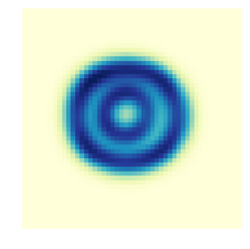
Barycenters with the sharp Sinkhorn. Using Algorithm 1 we can now apply the accelerated gradient descent approach proposed in [16] to find barycenters with respect to the sharp Sinkhorn distance. Figure 2 reports a qualitative experiment inspired by the one in [16], with the goal of comparing the two Sinkhorn barycenters. We considered images of random nested ellipses on a grid. We interpret each image as a distribution with support on pixels. The cost matrix is given by the squared Euclidean distances between pixels. Figure 2 shows some examples images in the dataset and the corresponding barycenters of the two Sinkhorn distances. While the barycenter of suffers a blurry effect, the barycenter is very sharp, suggesting a better estimate of the ideal one.


We conclude this section with a computational consideration on the two methods.
Remark 1 (Computations).
We compare the computational complexity of evaluating the gradients of and . Both gradients rely on the solution of the Sinkhorn problem in Equation 6, which requires operations to achieve an -accurate solution (this is easily derived from [1], see supplementary material). While the gradient of does not require further operations, the gradient of requires the inversion of an matrix as stated in Algorithm 1.
However, since the matrix to be inverted is a sum of a diagonal matrix and a low-rank matrix, the inversion requires operations (e.g. using Woodbury matrix identity), for a total cost of the gradient equal to .
Even for very large , Algorithm 1 is still efficient in all those settings where .
Moreover, note that the most expensive additional operations consist of matrix multiplications and the inversion of a positive definite matrix, which are very efficiently implemented on modern machines. Indeed, in our experiments the Sinkhorn algorithm was always the most expensive component of the computation. It is important to notice however that in practical applications both routines can be parallelized, and several ideas can be exploited to lower the computational costs of either algorithms depending on the problem structure (see for instance the convolutional Wasserstein distance in [32]). Therefore, depending on the setting, the computation of the gradient of the sharp Sinkhorn could be comparable or significantly slower than the regularized Sinkhorn or the automatic differentiation considered in [22].
5 Learning with Sinkhorn Loss Functions
Given the characterization of smoothness for both Sinkhorn distances, in this section we focus on a specific application: supervised learning with a Sinkhorn loss function. Indeed, the result of Theorem 2 will allow to characterize the statistical guarantees of an estimator devised for this problem in terms of its universal consistency and learning rates. Supervised learning with the (regularized) Sinkhorn loss was originally considered in [21], where an empirical risk minimization approach was adopted. In this work we take a structured prediction perspective [4]. This will allow us to study a learning algorithm with strong theoretical guarantees that can be efficiently applied in practice.
Problem Setting. Let be an input space and a set of histograms. As it is standard in supervised learning settings, the goal is to approximate a minimizer of the expected risk
| (17) |
given a finite number of training points independently sampled from the unknown distribution on . The loss function measures prediction errors and in our setting corresponds to either or .
Structured Prediction Estimator. Given a training set , we consider the structured prediction estimator proposed in [11], defined such that
| (18) |
for any . The weights are learned from the data and can be interpreted as scores suggesting the candidate output distribution to be close to a specific output distribution observed in training according to the metric . While different learning strategies can be adopted to learn the scores, we consider the kernel-based approach in [11]. In particular, given a positive definite kernel [3], we have
| (19) |
where is a regularization parameter while and are respectively the empirical kernel matrix with entries and the evaluation vector with entries , for any .
Remark 2 (Structured Prediction and Differentiability of Sinkhorn).
The current work provides both a theoretical and practical contribution to the problem of learning with Sinkhorn distances. On one hand, the smoothness guaranteed by Theorem 2 will allow us to characterize the generalization properties of the estimator (see below). On the other hand, Theorem 3 provides an efficient approach to solve the problem in Equation 18. Indeed note that this optimization corresponds to solving a barycenter problem in the form of Equation 10. Given the gradient estimation algorithm in Algorithm 1, this work allows to solve it by adopting first order methods such as gradient descent.
Universal Consistency of . We now characterize the theoretical properties of the estimator introduced in Equation 18. We start by showing is universally consistent, namely that it achieves minimum expected risk as the number of training points increases. To avoid technical issues on the boundary, in the following we will require for some to be the set of points with for any . The main technical step in this context is to show that for any smooth loss function on , the estimator in Equation 18 is consistent. In this sense, the characterization of smoothness in Theorem 2 is key to prove the following result, in combination with Thm. 4 in [11].
Theorem 4 (Universal Consistency).
Let , and be either or . Let be a bounded continuous universal11 1 This is a standard assumptions for universal consistency (see [35]). Example: . kernel on . For any and any distribution on let be the estimator in Equation 18 trained with points independently sampled from and . Then
| (20) |
The proof of Theorem 4 is reported in Appendix D. A result analogous to the one above was originally proved in [11] (Thm. 4) for a wide family of functions referred to as Structure Encoding Loss Function (SELF) (see [12] or the appendix of this work). While several loss functions used in structured prediction have been observed to satisfy this SELF definition, such characterization was not available for the Sinkhorn distances. The main technical step in the proof of Theorem 4 in this sense is to prove that any smooth function on satisfies the definition of SELF (see Definition 6 and Theorem 7 in the Appendix). Combining this result with Thm. in [11], we obtain that for every smooth loss function on the corresponding estimator in Equation 18 is universally consistent. The universal consistency of the Sikhorn distances is therefore guaranteed by the smoothness result of Theorem 2.
Theorem 4 guarantees to be a valid estimator for the learning problem. To our knowledge, this is the first result characterizing the universal consistency of an estimator minimizing (an approximation to) the Wasserstein distance.
Learning Rates. By imposing standard regularity conditions on the learning problem, it is possible to provide also excess risk bounds for . Since these conditions are quite technical, we provide here a brief overview while deferring an in-depth discussion to Appendix D.
We start from the observation (see e.g. Lemma in [11]) that the solution of the learning problem introduced in Equation 17 is such that
| (21) |
almost surely on . In particular corresponds to the minimizer of the conditional expectation of the loss with respect to given . As it is standard in statistical learning theory, in order to obtain generalization bounds for estimating we will impose regularity assumptions on the conditional distribution or, more precisely, on its corresponding conditional mean embedding ([34, 33]) with respect to a suitable space of functions.
Let be the kernel used for the estimation of the weights in Equation 19 and let be the associated reproducing kernel Hilbert spaces (RKHS) (see [3] for a definition). Let be the kernel on the output set . The RKHS associated to is , the Sobolev space of square integrable functions with smoothness (see e.g. [37]). We consider a function such that
| (22) |
almost surely on . For any , the quantity is known as the conditional mean embedding of in , originally introduced in [34, 33]. In particular, in [34] it was shown that in order to obtain learning rates for an estimator approximating , a key assumption is that belongs to , the tensor product between the space on the output and the space on the input. In this work we will require the same assumption.
It can be verified that is a RKHS for vector-valued functions [26, 25, 2] and that by asking we are requiring the conditional mean embedding of to be sufficiently regular as a function on . We are now ready to report our result on the statistical performance of .
Theorem 5 (Learning Rates).
Let , and be either or . Let and be a bounded continuous reproducing kernel on with associated RKHS . Let be the estimator in Equation 18 trained with training points independently sampled from and with . If defined in Equation 22 is such that , then
| (23) |
holds with probability for any , with a constant independent of and .
The proof of Theorem 5 requires to combine our characterization of the Sinkhorn distances (or more generally smooth functions on ) as structure encoding loss functions (see Theorem 7) with Thm. in [11] where a result analogous to the one above is reported for SELF loss functions. See Appendix D for a detailed proof.
Remark 3.
A relevant question is whether the Wasserstein distance could be similarly framed in the setting of structured prediction. However, the argument used to address Sinkhorn distances relies on their smoothness properties and cannot be extended to the Wasserstein distance, which is not differentiable. A completely different approach may still be successful and we will investigate this question in future work.
We conclude this section with a note on previous work. We recall that [21] has provided the first generalization bounds for an estimator minimizing the regularized Sinkhorn loss. In Theorem 5 however we characterize the excess risk bounds of the estimator in Equation 18. The two approaches and analysis are based on different assumptions on the problem. Therefore, a comparison of the corresponding learning rates is outside the scope of this work and is left for future research.
6 Experiments
We present here some experiments that compare the two Sinkhorn distances empirically. Optimization was performed with the accelerated gradient from [16] for and Bregman projections [5] for . The computation of barycenters with Bregman iteration is extremely fast compared to gradient descent. We have then used the barycenter of computed with Bregman projections as initial datum for gradient descent with : this has a positive influence on the number of iterations needed to converge and in this light the optimization with respect to the sharp Sinkhorn distance acts as a refinement of the solution with respect to .
| Support | ||||
| Improvement | 1% | 2% | 10% | 50% |
Barycenters with Sinkhorn Distances. We compared the quality of Sinkhorn barycenters in terms of their approximation of the (ideal) Wasserstein barycenter. We considered discrete distributions on bins, corresponding to the integers from to and a squared Euclidean cost matrix . We generated datasets of measures each, where only (randomly chosen) consecutive bins are different from zero, with the non-zero entries sampled uniformly at random between and (and then normalized to sum up to ). We empirically chose the Sinkhorn regularization parameter to be the smallest value such that the output of the Sinkhorn algorithm would be within from the transport polytope in 1000 iterations. Table 1 reports the absolute improvement of the barycenter of the sharp Sinkhorn distance with respect to the one obtained with the regularized Sinkhorn, averaged over independent dataset generation for each support size . As can be noticed, the sharp Sinkhorn consitstently outperforms its regularized counterpart. Interestingly, this improvement is more evident for measures with sparse support and tends to reduce as the support increases. This is in line with the remark in example Example 1 and the fact that the regularization term in tends to encourage oversmoothed solutions.
Learning with Wasserstein loss. We evaluated the Sinkhorn distances in an image reconstruction problem similar to the one considered in [38] for structured prediction. Given an image depicting a drawing, the goal is to learn how to reconstruct the lower half of the image (output) given the upper half (input). Similarly to [16] we interpret each (half) image as an histogram with mass corresponding to the gray levels (normalized to sum up to ). For all experiments, according to [11], we evaluated the performance of the reconstruction in terms of the classification accuracy of an image recognition SVM classifier trained on a separate dataset. To train the structured prediction estimator in Equation 18 we used a Gaussian kernel with bandwith and regularization parameter selected by cross-validation.
Reconstruction Error (%)
Classes
Hell[12]
KDE [38]
![[Uncaptioned image]](1805.11897v1/datasetcrop.png) Figure 3: Average reconstruction errors of the Sinkhorn, Hellinger, and KDE estimators on the Google QuickDraw reconstruction problem. On the right, a mini-sample of the dataset.
Figure 3: Average reconstruction errors of the Sinkhorn, Hellinger, and KDE estimators on the Google QuickDraw reconstruction problem. On the right, a mini-sample of the dataset.
Google QuickDraw. We compared the performance of the two estimators on a challenging dataset. We selected classes from the Google QuickDraw dataset [23] which consists in images of size pixels. We trained the structured prediction estimators on images per class and tested on other images. We repeated these experiments times, each time randomly sampling a different training and test dataset. Figure 3 reports the reconstruction error (i.e. the classification error of the SVM classifier) over images reconstructed by the Sinkhorn estimators, the structured prediction estimator with Hellinger loss [11] and the Kernel Dependency Estimator (KDE) [38]. As can be noticed, both Sinkhorn estimators perform significantly better than their competitors (except the Hellinger distance outperforming on 4 classes). This is in line with the intuition that optimal transport metrics respect the way the mass is distributed on images [15, 16]. Moreover, it is interesting to note that the estimator of the sharp Sinkhorn distance provides always better reconstructions than its regularized counterpart, supporting the idea that it is more suited to settings where Wasserstein distance should be used.
The experiments above are a preliminary assessment of the potential of sharp Sinkhorn distance in barycenters and learning settings. More extensive experiments on real data will be matter of future work.
7 Discussion
In this paper we investigated the differential properties of Sinkhorn distances. We proved the smoothness of the two functions and derived an explicit algorithm to efficiently compute the gradient of the sharp Sinkhorn distance. Our result allows to employ the sharp Sinkhorn distance in applications that rely on first order optimization methods, such as in approximating Wasserstein barycenters and supervised learning on probability distributions. In this latter setting, our characterization of smoothness allowed to study the statistical properties of the Sinkhorn distance as loss function. In particular we considered a structured prediction estimator for which we proved universal consistency and generalization bounds. Future work will focus on further applications and a more extensive comparison with the existing literature.
References
- [1] J. Altschuler, J. Weed, and P. Rigollet. Near-linear time approximation algorithms for optimal transport via sinkhorn iteration. In NIPS, pages 1961–1971, 2017.
- [2] M. A. Alvarez, L. Rosasco, N. D. Lawrence, et al. Kernels for vector-valued functions: A review. Foundations and Trends® in Machine Learning, 4(3):195–266, 2012.
- [3] N. Aronszajn. Theory of reproducing kernels. Transactions of the American mathematical society, 68(3):337–404, 1950.
- [4] G. Bakir, T. Hofmann, B. Schölkopf, A. Smola, B. Taskar, and S. Vishwanathan. Predicting structured data. neural information processing, 2007.
- [5] J. Benamou, G. Carlier, M. Cuturi, L. Nenna, and G. Peyré. Iterative bregman projections for regularized transportation problems. SIAM J. Scientific Computing, 37(2), 2015.
- [6] Y. Bengio. Gradient-based optimization of hyperparameters. Neural computation, 12(8):1889–1900, 2000.
- [7] A. Berlinet and C. Thomas-Agnan. Reproducing kernel Hilbert spaces in probability and statistics. Springer Science & Business Media, 2011.
- [8] D. Bertsimas and J. Tsitsiklis. Introduction to Linear Optimization. Athena Scientific, 1st edition, 1997.
- [9] N. Bonneel, G. Peyré, and M. Cuturi. Wasserstein barycentric coordinates: histogram regression using optimal transport. ACM Trans. Graph., 35(4):71–1, 2016.
- [10] O. Chapelle, V. Vapnik, O. Bousquet, and S. Mukherjee. Choosing multiple parameters for support vector machines. Machine learning, 46(1-3):131–159, 2002.
- [11] C. Ciliberto, L. Rosasco, and A. Rudi. A consistent regularization approach for structured prediction. In D. D. Lee, M. Sugiyama, U. V. Luxburg, I. Guyon, and R. Garnett, editors, Advances in Neural Information Processing Systems 29, pages 4412–4420. Curran Associates, Inc., 2016.
- [12] C. Ciliberto, A. Rudi, L. Rosasco, and M. Pontil. Consistent multitask learning with nonlinear output relations. In Advances in Neural Information Processing Systems, pages 1983–1993, 2017.
- [13] R. Cominetti and J. S. Martín. Asymptotic analysis of the exponential penalty trajectory in linear programming. Mathematical Programming, 67(1):169–187, Oct 1994.
- [14] N. Courty, R. Flamary, and D. Tuia. Domain adaptation with regularized optimal transport. In ECML/PKDD 2014, LNCS, pages 1–16, Nancy, France, Sept. 2014.
- [15] M. Cuturi. Sinkhorn distances: Lightspeed computation of optimal transport. In C. J. C. Burges, L. Bottou, M. Welling, Z. Ghahramani, and K. Q. Weinberger, editors, Advances in Neural Information Processing Systems 26, pages 2292–2300. Curran Associates, Inc., 2013.
- [16] M. Cuturi and A. Doucet. Fast computation of wasserstein barycenters. In E. P. Xing and T. Jebara, editors, Proceedings of the 31st International Conference on Machine Learning, volume 32 of Proceedings of Machine Learning Research, pages 685–693, Bejing, China, 22–24 Jun 2014. PMLR.
- [17] M. Cuturi and G. Peyré. A smoothed dual approach for variational wasserstein problems. SIAM J. Imaging Sciences, 9(1):320–343, 2016.
- [18] S. Dempe. Foundations of bilevel programming. Springer Science & Business Media, 2002.
- [19] C. Edwards. Advanced Calculus of Several Variables. Dover Books on Mathematics. Dover Publications, 2012.
- [20] R. Flamary, M. Cuturi, N. Courty, and A. Rakotomamonjy. Wasserstein discriminant analysis. Machine Learning, May 2018.
- [21] C. Frogner, C. Zhang, H. Mobahi, M. Araya-Polo, and T. Poggio. Learning with a wasserstein loss. In Proceedings of the 28th International Conference on Neural Information Processing Systems - Volume 2, NIPS’15, pages 2053–2061, Cambridge, MA, USA, 2015. MIT Press.
- [22] A. Genevay, G. Peyré, and M. Cuturi. Learning generative models with sinkhorn divergences. In International Conference on Artificial Intelligence and Statistics, pages 1608–1617, 2018.
- [23] I. Google. QuickDraw Dataset. 2017. Available on line.
- [24] T. Kollo and D. von Rosen. Advanced Multivariate Statistics with Matrices. Mathematics and Its Applications. Springer Netherlands, 2006.
- [25] G. Lever, L. Baldassarre, S. Patterson, A. Gretton, M. Pontil, and S. Grünewälder. Conditional mean embeddings as regressors. In International Conference on Machine Learing (ICML), volume 5, 2012.
- [26] C. A. Micchelli and M. Pontil. On learning vector-valued functions. Neural computation, 17(1):177–204, 2005.
- [27] V. Moretti. Spectral Theory and Quantum Mechanics: With an Introduction to the Algebraic Formulation. UNITEXT. Springer Milan, 2013.
- [28] G. Peyré, M. Cuturi, et al. Computational optimal transport. Technical report, 2017.
- [29] A. Rolet, M. Cuturi, and G. Peyré. Fast dictionary learning with a smoothed wasserstein loss. In A. Gretton and C. C. Robert, editors, Proceedings of the 19th International Conference on Artificial Intelligence and Statistics, volume 51 of Proceedings of Machine Learning Research, pages 630–638, Cadiz, Spain, 09–11 May 2016. PMLR.
- [30] M. A. Schmitz, M. Heitz, N. Bonneel, F. Ngole, D. Coeurjolly, M. Cuturi, G. Peyré, and J.-L. Starck. Wasserstein dictionary learning: Optimal transport-based unsupervised nonlinear dictionary learning. SIAM Journal on Imaging Sciences, 11(1):643–678, 2018.
- [31] R. Sinkhorn and P. Knopp. Concerning nonnegative matrices and doubly stochastic matrices. Pacific J. Math., 21(2):343–348, 1967.
- [32] J. Solomon, F. De Goes, G. Peyré, M. Cuturi, A. Butscher, A. Nguyen, T. Du, and L. Guibas. Convolutional wasserstein distances: Efficient optimal transportation on geometric domains. ACM Transactions on Graphics (TOG), 34(4):66, 2015.
- [33] L. Song, K. Fukumizu, and A. Gretton. Kernel embeddings of conditional distributions: A unified kernel framework for nonparametric inference in graphical models. IEEE Signal Process. Mag., 30(4):98–111, 2013.
- [34] L. Song, J. Huang, A. Smola, and K. Fukumizu. Hilbert space embeddings of conditional distributions with applications to dynamical systems. In Proceedings of the 26th Annual International Conference on Machine Learning, pages 961–968. ACM, 2009.
- [35] I. Steinwart and A. Christmann. Support vector machines. Springer Science & Business Media, 2008.
- [36] C. Villani. Optimal Transport: Old and New. Grundlehren der mathematischen Wissenschaften. Springer Berlin Heidelberg, 2008.
- [37] H. Wendland. Scattered data approximation, volume 17. Cambridge university press, 2004.
- [38] J. Weston, O. Chapelle, A. Elisseeff, B. Schölkopf, and V. Vapnik. Kernel dependency estimation. In Advances in Neural Information Processing Systems 15, pages 873–880, Cambridge, MA, USA, Oct. 2003. Max-Planck-Gesellschaft, MIT Press.
- [39] J. Ye, P. Wu, J. Z. Wang, and J. Li. Fast discrete distribution clustering using wasserstein barycenter with sparse support. IEEE Transactions on Signal Processing, 65(9):2317–2332, May 2017.
Supplementary Material
Appendix A Barycenter of Dirac Deltas
Wasserstein barycenter problems can be divided into two main classes: problems in which the support is free (and must be computed, generating a nonconvex problem [16]) and problems where the support is fixed. In some cases, the latter is the only valid choice: for instance, when the geometric domain is a space of symbols and the cost matrix contains the symbol-to-symbol dissimilarities, no extra information of the symbol space is available and the support of the barycenter will have to lie on a pre-determined set in order to be meaningful. A concrete example is the following: when dealing with histograms on words, the barycenter will optimize how to spread the mass among a set of known words that are used to build the matrix , through a operation. In the following we carry out the computation of the barycenter of two Dirac deltas with regularized Sinkhorn and Sinkhorn distances, in order to prove what stated in example 1.
Barycenter with :
Let be the Dirac delta centered at and the Dirac delta centered at . We fix the set of admissible support of the barycenter , where for any . For the sake of simplicity let us assume that contains the point . The cost matrices with mutual distances between and and and will be
Since the support is fixed, only the masses of the barycenter are to be computed. Vector is the minimizer of the following functional
Note that since Dirac delta has mass 1 concentrated at a point, the transport polytope corresponding to and a Dirac delta is . The elements in are those matrices such that and . Thus,
| (24) |
which implies . In this case, contains only one matrix, which coincides with . The distance is given by and, similarly, . Then, the goal is to minimize
with the constraint that . The partial derivative with respect to is given by
Setting it equal to zero, it yields . The constraint leads to
Then the barycenter has masses where each is strictly positive, with maximum at the entry corresponding to the point which realizes the minimum distance from and , i.e. . The sparsity of the initial deltas is lost.
Barycenter with :
On the other hand, let us compute the barycenter between and with respect to the Sinkhorn distance recalled in Eq. (7). The very same considerations on still hold, so contains only. Hence, in this case the Sinkhorn barycenter functional coincides with the Wasserstein barycenter functional , since , for . This trivially implies that .
Appendix B Proof of Proposition 1 in section 3
See 1
Proof.
As shown in [13](Prop.5.1), the sequence converges to an optimal plan of W as goes to infinity. More precisely,
exponentially fast, that is . Thus,
As for the second part, let be the . By optimality of and for their optimization problems, it holds
Indeed, since is the optimum, it attains the minimum and hence
for any other , including . By definition of and W, the inequalities above can be rewritten as
which goes to with speed as goes to infinity. ∎
Appendix C Proofs on differential properties and formula of the gradient
Proof.
Let us show the proof for first. We organize it in three steps:
Step 1. is smooth when is: when considering histograms, depends on its argument and through the optimal coupling , being the cost matrix fixed. Thus, since is a smooth function of (being the Frobenius product of with a constant matrix), showing that is smooth in amounts to showing that is smooth.
Step 2. is smooth when is: By Sinkhorn’s scaling theorem [31], the optimal plan is characterized as follows
| (25) |
Being the exponential a smooth function, is smooth in and if the dual optima and are. Our goal is then showing smoothness with respect to and of the dual optima.
Step 3. is smooth in : this is the most technical part of the proof. First of all, let us stress that one among the rows/columns constraints of is redundant: the standard dual problem recalled in Equation 12 has an extra dual variable, and this degree of freedom is clear noticing that if is feasible, than the pair is also feasible. In the following, we get rid of the redundancy removing one of the dual variables. Hence, let us set
where corresponds to with the last element removed.
To avoid cumbersome notation, from now on we denote and . The function is smooth and strictly convex in : hence, for every fixed in the interior of there exist such that . We now fix and show that is on a neighbourhood of .
Set ; the smoothness of ensures that . Fix such that . Since and is strictly convex, is invertible. Then, by the implicit function theorem, there exist a subset and a function such that
- i)
- ii)
- iii)
.
For each in , since is a stationary point for and is strictly convex, then , which is- recalling the notation set before- . By a standard covering argument, is on the interior of . As this holds true for any , the optima , and hence , are on the interior of .
Let us now focus on the smoothness of . Note that when belong to the interior of the simplex, all components are strictly positive. From the characterization of recalled in Equation 25, we know for any . Then, since the logarithm is a smooth function of , the term is smooth in and . This fact combined with the first part of the proof shows the smoothness of . ∎
With a similar procedure, the implicit function theorem provides a formula for the gradient of sharp Sinkhorn distance. See 3
Proof.
Let us adopt the same notation as in the previous proof. Since , by a direct computation, can be written as
where is the matrix given by and is the matrix with column removed. In the following, we keep track of the dependence on only. Being the gradient of , and a stationary point, we have
| (26) |
For the sake of clarity, notice that:
- i)
;
- ii)
, as we are considering it is a function of , , ;
- iii)
;
- iv)
, , thus .
Our goal is to derive : by matrix differentiation rules [24] and Equation 26,
| (27) |
Let us analyse each term: is matrix with identity and zeros block, and is the Hessian of evaluated at , which is a matrix. Together with Equation 27, this yields
For the sake of clarity, note that and contains the gradients of the components as columns, i.e.
Now, since and corresponds to Equation 25 a straightforward computation shows that
Setting , then the formula above can be rewritten as
which is exactly
Since by definition, the gradient belongs to the tangent space of the domain, and , we project on the tangent space of the simplex, recovering ∎
C.1 Massaging the gradient to get an algorithmic-friendly form
In the proof of theorem 3 we have derived a formula for the gradient of Sinkhorn distance. In this section we further manipulate it in order to obtain an algorithmic friendly expression that also points out some interesting bits that were hidden in the formula above. All the notation has already been introduced: from now on, we will drop the and denote the optimal plan by to make the notation neater.
An explicit computation of the second derivatives of with respect to and for and leads to the following identity
That is, is a block matrix and each block can be expressed in terms of the plan . The block structure can be exploited when it comes to compute the inverse: we have shown that the gradient of the dual potentials is given by
Now, the inverse of a block matrix is again a block matrix, say
Then, . By the formula of the block inverse, setting
the blocks and are given by
Note that is symmetric and so its inverse. Now, we can rewrite , with , as
and we conclude that
Comment on Remark 1:
In the recent work [1], it has been shown that Sinkhorn-Knopp algorithm outputs a matrix whose distance from the transport polytope is smaller than in iterations, where and . Let us denote by and the maximum and minimum elements of respectively. Then,
This yields the lower bound
where is a constant independent of . We can then conclude that Sinkhorn-Knopp algorithm returns a matrix such that
in .
Appendix D Proofs in 5: Learning with Sinkhorn Loss Functions
We recall the main definition and tools from [11] needed to fully understand what discussed in section 5. The structured prediction estimator recalled in Equation 18 is derived in [11] for a large class of loss functions that are referred to as Structure Encoding Loss Functions (SELF) and satisfy the following assumption:
Definition 6 (SELF).
Let be a set. A function is a Structure Encoding Loss Function (SELF) if there exists a separable Hilbert space with inner product , a continuous map and a bounded linear operator such that
| (28) |
While in [11] it has been observed that a wide range of commonly used loss functions are SELF, no such result was known for Sinkhorn loss. This work also provides an answer to this question. In this direction, let us show a first result on smooth function, which will be a key tool in the rest of the analysis. Note that we will use the notation for the Sobolev space .
Theorem 7.
(Smooth functions are SELF) Let . Any function such that is SELF.
Proof.
By assumption . Since is compact,
| (29) |
for .The Sobolev space is a Reproducing Kernel Hilbert Space (RKHS) [7] and we denote by the reproducing kernel. The product space is also an RKHS with reproducing kernel , i.e. in general . Since , by reproducing property there exists a function such that
By the isometric isomorphism [27], with the space of Hilbert-Schmidt operators from to itself, it holds
| (30) |
where is the adjoint operator of . To meet the conditions of definition 6 it remains to show that and are bounded. But is bounded in for any by definition of reproducing kernel and the operator norm is bounded from above by the Hilbert-Schmidt norm which is trivially bounded since . ∎
Corollary 8.
The regularized and sharp Sinkhorn losses and are SELF.
Proof.
Since is compact and , are in the interior on by Thm. 2, a direct application of the result above shows that and are SELF. ∎
Proof.
Since , are SELF function and is compact, the result follows from Thm. 4 in [11]. ∎
We conclude the section with some comments on Thm. 5 and its proof. We have shown that and are SELF and can be written as
| (31) |
with the reproducing kernel of the Sobolev space . See 5
Proof.
The proof substantially takes advantage of the fact that and are SELF and inherits the generalization bounds proved in Thm. 5 in [11]. ∎
Remark 4.
A relevant question is whether the Wasserstein distance could be similarly framed in the setting of structured prediction. However, the argument used to address Sinkhorn distances relies on their smoothness properties and cannot be extended to the Wasserstein distance, which is not differentiable. A completely different approach may still be successful and we will investigate this question in future work.
Appendix E Experiment on MNIST
This last section is a short supplement to section 6. We present a small experiment on the MNIST dataset that has the same flavour as the experiment on GoogleQuickDraw dataset but adresses a more specific target: to evaluate better the quality of the prediction rather than the overall quality of the reconstructed image, we train the SVM classifier trained on a separate dataset made of examples of lower halves of digits . Since the classificator is trained on lower halves only, we have selected a subset of digits with clearly diverse shapes, to disregard any legitimate vagueness. This means that any classification errors will be due to a poor prediction of the lower half.
We performed the reconstruction with both and loss. We tested the performance of the two estimators on examples. Figure 4 reports the performance of the two estimators, as follows:
- i)
the terms on the diagonal presents the number of misclassification of the lower half predicted with and losses;
- ii)
the number on the upper diagonal represents the number of errors occurred in the classification of the prediction with on those examples that were correctly classified when reconstructed with ;
- iii)
conversely, the number on the lower diagonal represents the number of errors occurred in the prediction with on those examples that were correctly classified when reconstructed with .
To be more precise, denote by the vector with labels predicted by the classifier when tested on the halves of digits predicted with loss and analogously the vector with labels given by the classifier tested on the halves of images predicted with loss. Vector L is the vector with the true labels of the test set. Consider two vectors and defined as follows:
Table in Fig. 4 corresponds to
What we observed is the following: since the classifier was trained and tested on the lower halves only, the blurriness in the reconstruction performed with played a substantial role in the misclassification on digit in favour of digit . On the other hand, the sharpness of the reconstruction with is a major advantage for the correct classification.
err
![[Uncaptioned image]](1805.11897v1/5wlambda.png)
![[Uncaptioned image]](1805.11897v1/5wtilde.png) Figure 4: (Right) Relative error (see text) for the Sinkhorn estimators on the digit reconstruction problem. (Left) Sample predictions for egularized (First image) and sharp Sinkhorn estimators.
Figure 4: (Right) Relative error (see text) for the Sinkhorn estimators on the digit reconstruction problem. (Left) Sample predictions for egularized (First image) and sharp Sinkhorn estimators.