A Markov Chain Model for the Cure Rate of Non-Performing Loans
Abstract
A Markov-chain model is developed for the purpose estimation of the cure rate of non-performing loans. The technique is performed collectively, on portfolios and it can be applicable in the process of calculation of credit impairment. It is efficient in terms of data manipulation costs which makes it accessible even to smaller financial institutions. In addition, several other applications to portfolio optimization are suggested.
Key words: Cure Rate Estimation, Markov Chains, Survival Analysis, IFRS 9 Provisioning.
2010 Mathematics Subject Classification: 62M05, 62N02, 91B70
JEL Classification: G21, M41
Introduction
In calculating the credit impairment the IFRS 9 standard permits, under certain conditions, the usage of cure rate in order to reduce the amount of bank provisions. The logic behind this allowance is, that if an impaired amount will eventually return to regular status, the bank need not calculate provisions on it. Several methodological manuals are available to the banking community which (cf. e.g. [2]), often without stipulation on the assumptions on the model, provide recipes for calculation of a cure rate. Estimates made in this way turn out to be often overly conservative and, sometimes, dissatisfactory, because the basic assumptions of the model could not be verified. The presented technique allows to calculate with any desired accuracy and any desired frequency. (E.g., monthly, quarterly, etc.) The model uses data only from the past 12 months in order to provide a most recent measurement of the cure rate. This is, sometimes, required by regulators for financial quantities measured collectively. This very fact is the reason why in low-default portfolios, which are often those found in small banks, the results of this type of method do not satisfy even very basic assumptions about the cure rate in general. For this reason we apply a smoothing method from Survival analysis. This method is the topic of Section 3.
The usage of Markov-chain models, in general, is a technique accessible to the banking management and is part of their routine in accessing credit risk and expected credit losses, several studies document and contribute to this practice, including [3], [4] and [5]. It appears that Monte Carlo techniques similar to those demonstrated in e.g., [6] are applicable in the study of cure rate and it is my belief that future interest in this subject would move in this direction.
In Section 4 we produce two numerical examples using data form three small Bulgarian banks11 1 Bulgarian banks are bound to report expected credit losses and to calculate provisions based on IFRS 9 since 01/01/2018. They are, in general, computing cure rates for their retail loan portfolios and for other portfolios of standardized products..
In addition, in Section 5 we show how this method provides several tools to identify some portfolios where cure rate is inapplicable, but rather a different managerial approach will be more successful.
I wish to thank my colleagues Jana Kostova and Alessandro Merlini from ASTOR BG Consulting for bringing this problem to my attention and for providing the data for the actual computations.
1 Cure Rate
Cure rate is meant to measure the propensity of loans to return to regular status after they have been found delinquent. In a portfolio, collectively, the cure rate estimates what proportion of non-performing loans will be, in the end, repaid. Given the possibility of a loan which is once “cured” to relapse or to move back and forth between categories it is not enough to simply measure the proportion over a certain horizon of time.
For the purposes of this study we assume that a loan is considered non-performing after it is found more than 90 days late. We make the following assumptions
- 1.
The loan is finally cured after it becomes less than one month past due.
- 2.
Loans which are N or more months past due are considered lost and are written off.
- 3.
We should distinguish performing loans which have been granted forbearance. According to [1] these would be loans to parties experiencing financial difficulties in meeting their obligations and the bank has agreed to offer them special contractual terms. If such loan preserves its regular status for a year we consider it cured, otherwise we consider it lost.
- 4.
States are assigned to all loans in the portfolio, based on , the whole number of months past-due at time . The state where is an absorbing state, as well as the one with . The forborne loans are assigned in a separate state. Hence, the number of states is .
- 5.
We assume the time periodicity of observation to the loan tape is annual. We measure the probabilities of transition between states by observing the migration between states within a year prior to time .
- 6.
We assume that the migration in the previous years is irrelevant to the further development of the portfolio. Moreover, we assume that transition rates do not vary in time.
Assumptions 1-3 are a question of bank policy and, although they satisfy the requirement of IFRS 9, an alternative configuration may be set. Assumption 5 is inessential, although it should be noted that small banks often have shallow, low-default portfolios and high frequency observation leads to volatile cure rates.
2 Markov Process
For a typical loan of the considered portfolio we have thus constructed a finite Markov chain of random variables , which take as value the state of the loan at year . It has states , describing the state the loan is. With an appropriate ordering we can assume that denotes the state where , denotes , is the forborne state and, for any , the state is characterized by . Hence, is the first non-performing state, corresponding to .
- •
Assumption 6 form Section 1 implies time homogeneity.
- •
Assumptions 1 and 2 imply that and are absorbing states and, hence, they form, each by itself two recurrent communication classes.
- •
If any part of the set of states forms a recurrent class this would imply that the loan contract for this particular portfolio can be optimized. We are giving an example to illustrate this in Section 4. For this reason we assume that is the set of transitive states.
- •
Assumption 3 implies that is a transitive. In fact,
where and , satisfying are the probabilities to survive and fail, respectively.
We write the transition matrix , therefore as follows:
Furthermore, for the limit matrix we have:
where is the zero matrix. For the matrix we have
where and satisfy and are the probabilities of a loan showing months of payment delay to be cured or lost, respectively. Hence, in search for the cure rate, our goal is to study the vector .
Proposition 1.
In the notation defined above, the probability to cure for a loan which is months past due at time can be found on the th row of the first column of the matrix
Proof.
Since is a substochastic matrix, representing the transition rates of transitive states, we know that as . For this reason the matrix , with — the identity matrix of size is, indeed, invertible.
Denote by the probability of a loan with initial state to reach eventually the state , . (In the notation above, these are the entries of the matrix , , and .) We have
That is,
Hence
∎
3 Survival Model
Let be probability of a loan to be cured if the initial state is at least months past due. For non-preforming states, ,
This function needs to satisfy the following conditions:
- 1.
- 2.
for
- 3.
is non-increasing.
In addition, one would expect that chances of failure would increase as a function of , the months past-due. This is due, in part, to two reasons. First, the longer delay signifies a more dire economic status. And second, portfolio manager would make more effort to increase the opportunities of survival of these loans which are less in delay, since they have better chance. This gives us an extra condition
- 4
The logarithmic derivative is decreasing.
Generally the outcome of calculating the Markov chain need not satisfy these conditions. In order to smoothen the results we apply tools form the Survival Analysis. (Cf. e.g. [7].) A common choice of survival function is a best-fitting Weibull curve:
corresponding to a Weibull distribution with CDF . Condition 4 simply means that the hazard rate is an increasing function which would imply that the shape parameter of the curve satisfies . The parameters and must be chosen by fitting the CDF of this distribution to the points
After this, the cure rate of the portfolio is equal to .
4 Numerical Examples
Example 4.1.
A Credit-Card Portfolio
We now consider the portfolio of select credit cards from a small bank
at the end of March 2007. The total size of the portfolio is
€328.9 Thousand,
consisting of 1185 loans. The bank management assumes that a loan not
serviced for
8 or more months is lost, . The transition matrix , according
to the
notation above is:
Next, we compute the matrices :
and :
Next we fit a Weibull curve on ten points:
using a linear regression. The results are shown in Table 1.
The shape coefficient is different from 0 at the 99% level of significance. The one-sided hypothesis for is rejected at the 95% level33 3 The -value of the one-sided Wald test comes to 0.049. . The expected cure rate is computed as .
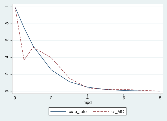
Figure 1 shows the cure rate computed from the survival function compared with the raw Markov chain results.
Example 4.2.
A State-Owned-Corporations Portfolio
A portfolio of select corporate loans to state-owned corporations was tested for cure rate. The portfolio consists of 97 loans with total value €892.8 Thousand. All measurements are taken at the end of March 2017.
The transition matrix is as follows:
Notice, that states , and form a separate recurrent communication class and, hence, is not a transitive state. The current cure-rate model is inapplicable for this portfolio44 4 Most banks in Bulgaria are avoiding the use cure rate for corporate portfolios.. In fact we conclude that there is a pattern of loans cycling between these three states without ever being lost or cured.
5 Portfolios optimization
5.1 Cyclicity
As seen in Example 4.2, it is possible to find a recurrent class which contains both performing and non-performing states. This is an indication that loans with this risk profile may oscillate between performance and non-performance without ever becoming cured or lost. Instead of trying to remedy the situation using cure rate the management should seek to optimize the contract for this type of loans.
5.2 Hazard rate
Example 4.1 shows how the hazard rate might turn out constant. In fact, a large part of the tested portfolios of this type exhibited statistically indistinguishable from 1.
This may be due simply to the shallowness of the portfolio, however, it may indicate that young loans die unnecessarily quickly. Therefore, it may be worth for the bank management to consider contractual change in order to better channel the behavioral patterns of their clients.
5.3 Time to failure or recovery
This model allows to compute expected time it takes for a loan in state to be resolved, i.e., to either fail, or cure.
Proposition 2.
The time to absorption of a transitive state , , can be obtained by summing the entrees of the corresponding row (i.e., the st row) of the matrix .
Proof.
One can see that that is the sum
where is the expected time a state spends in state starting initial state . Moreover, taking into account that
a simple computation shows, is the element of that matrix which stays in st row and st column. ∎
Proposition 2 produces a tool for estimation of the expected period of uncertainty for loans. Furthermore, in a similar fashion one can develop a early-warning system for prognosticating potential non-performing loans, by computing the times and , etc.
6 Conclusions
I suggest a Markov-chain model which, together with a survival model, can be used to estimate the cure rate in a portfolio of loans with homogeneous risk. 55 5 The model was subsequently tested by computing cure rates for various select subportfolios of the retail product line over a period in years 2015-2016. The data was obtained from three small Bulgarian banks. The analysis produced cure rates ranging between 3-22%. These results appear in line with the guidance of [1].
Furthermore, we show that this technique produces the following instruments can be of use for making these portfolios more efficiently.
- 1.
One can test if the portfolio demonstrates cyclical behavior, which defeats the purpose of computation of CR.
- 2.
One can compute the hazard-rate function of the portfolio and study it for further portfolio optimization, particularly in cases of unexpected hazard rate.
- 3.
Expected time-to-resolution together with probabilities of default may be used for monitoring loans which are past-due over an extended period.
- 4.
Expected time-to-NPL can be computed to aid the development of an early warning system.
References
- [1] Asset Quality Review, Phase 2 Manual, ECB 2014.
- [2] Basel Committee on Banking Supervision Prudential treatment of problem assets — definitions of non-performing exposures and forbearance, Consultative Document. BIS, July 15, 2016.
- [3] Gaffney, E., R. Kelly, and F. McCann, (2014), A transitions-based framework for estimating expected credit losses, Research Technical Papers 16/RT/14, Central Bank of Ireland.
- [4] Grimshaw, S. D. and Alexander, W. P. (2011), Markov chain models for delinquency: Transition matrix estimation and forecasting. Appl. Stochastic Models Bus. Ind., 27: 267-279. doi:10.1002/asmb.827
- [5] Robert A. Jarrow, David Lando, and Stuart M. Turnbull (2008) A Markov Model for the Term Structure of Credit Risk Spreads. Financial Derivatives Pricing: pp. 411-453.
- [6] Todorov, V. and Dimov, I. T. (2016) Monte Carlo methods for multidimensional integration for European option pricing, AIP Conference Proceedings, 1773:1, 100009, doi:10.1063/1.4965003.
- [7] Weibull, W. (1951) A Statistical Distribution Function of Wide Applicability. Journal of Applied Mechanics, 18, 293-297.
Institute of Mathematics and Informatics, Bulgarian Academy of Sciences, Acad. G. Bonchev Str., Block 8, 1113 Sofia, Bulgaria
E-mail address: vboutcha@math.bas.bg